This post discusses how you can get horseshoe-looking patterns (sometimes also called cyclic, or U- or V-shaped) in common dimension reduction methods, from data that are generated by processes that have little to do with horseshoes, cycles, Us or Vs.

1 Diaconis, Goel and Holmes

In their paper “Horseshoes in multidimensional scaling and local kernel methods” in The Annals of Applied Statistics (2008), Vol. 2, page 777 (DOI: 10.1214/08-AOAS165), Diaconis, Goel and Holmes looked at situations in which the distance matrix of a set of objects is concentrated along the diagonal (see Figure 1, upper left panel). They set out from the example of the voting records of the members of the 2005 United States House of Representatives. From these records, they computed all pairwise distances (or dissimilarities), applied classical multi-dimensional scaling, and observed a horseshoe pattern.

Generalizing this, and following the ideas of Diaconis, Goel and Holmes, consider a set of objects whose (dis)similarities are described by the matrix of pairwise distances $D$. In particular, consider the idealised situation of matrices like the following one. The elements of $D$ are 0 along the diagonal, and the values increase with the distance from the diagonal, with some rate $\lambda^{-1}$, until they saturate at some maximum value, which w.l.o.g. we can set to 1:

\[ D_{ij} = 1 - e^{\displaystyle -\lambda | i-j |} \] where $n$ is a positive integer, $i,j=1,\ldots,n$, and $D$ is an $n\times n$ matrix.

set.seed(0xbedada)
library("conflicted")
library("dplyr")
library("ggplot2")
library("gridExtra")
library("reshape2")
library("ggfortify")
library("Rtsne")
library("umap")

plotMatrixAsImage <- function(x) {
  ggplot(melt(x), aes(x = Var1, y = Var2, fill = value)) + geom_tile() + 
    scale_fill_gradient2() +
    ggtitle(deparse(substitute(x))) + coord_fixed() + xlab("") + ylab("") +
    theme(plot.title = element_text(hjust = 0.5))
}

plotMDS <- function(x, tit, flipy) {
  dat <- as_tibble(`colnames<-`(x, c("P1", "P2"))) 
  if (tit %in% flipy)
    dat <- mutate(dat, P2 = -P2)
  ggplot(dat) + 
    geom_point(aes(x = P1, y = P2)) + coord_fixed() + 
    ggtitle(tit) +
    theme(plot.title = element_text(hjust = 0.5)) +
    expand_limits(y = c(-1, 1) * 0.2 * max(abs(dat$P1)))
}

variousMDSPlots <- function(..., perplexity = 30, flipy = character(0)) { 
  grid.arrange(
    plotMatrixAsImage(...), 
    plotMDS(stats::cmdscale(...), "cmdscale", flipy),
    plotMDS(MASS::isoMDS(...)$points, "isoMDS", flipy),
    plotMDS(Rtsne(..., is_distance = TRUE, perplexity = perplexity)$Y, "t-SNE", flipy),
    plotMDS(umap::umap(..., input = "dist")$layout, "UMAP", flipy),
    layout_matrix = rbind(c(1, 2, 3), c(1, 4, 5))
  )
}

diaconisMatrix <- function(lambda, n)
  1 - outer(seq(0, 1, length.out = n), seq(0, 1, length.out = n), 
        FUN = function(a, b) exp(-lambda * abs(a-b)))

D <- diaconisMatrix(lambda = 2, n = 100)

variousMDSPlots(D)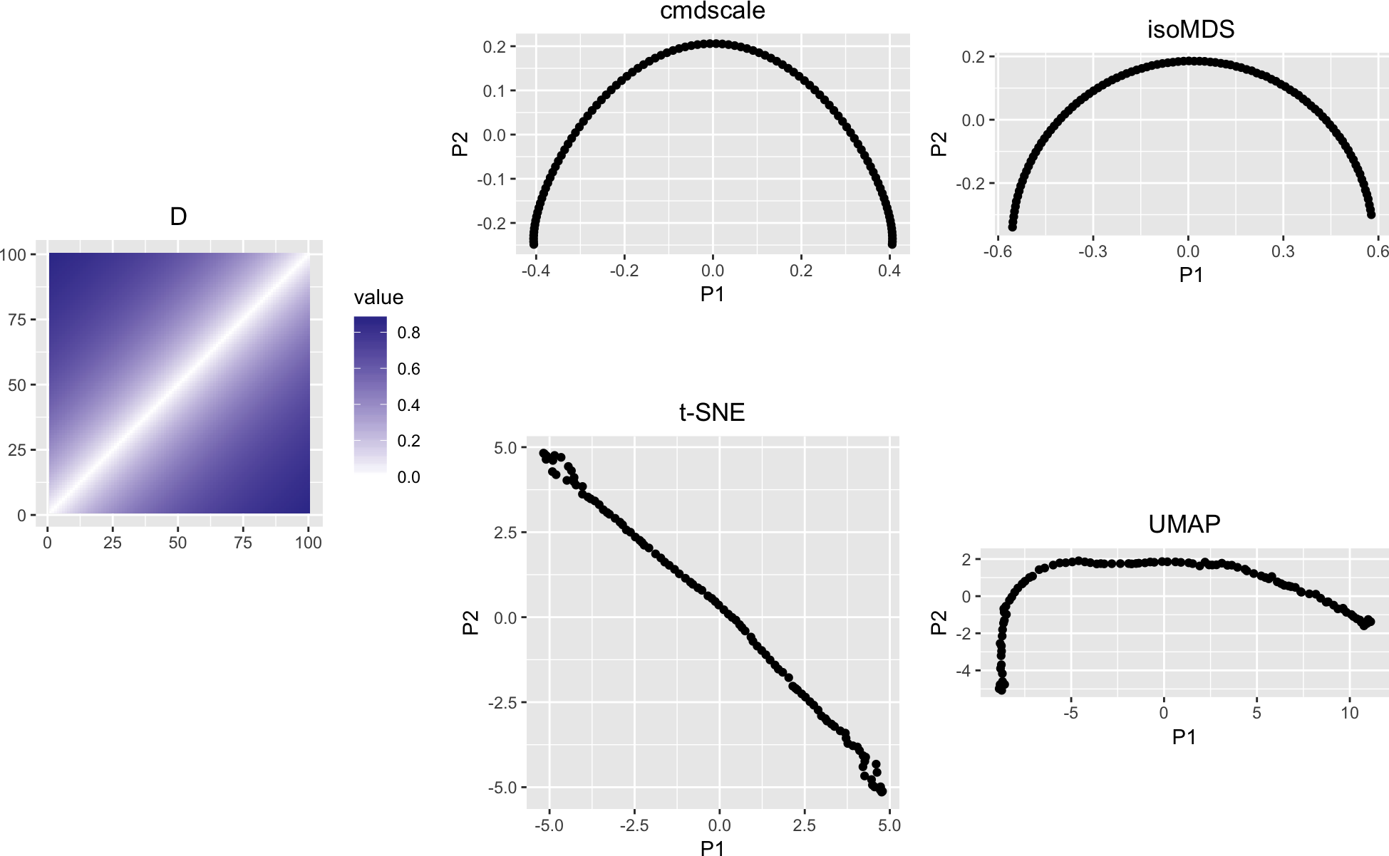

The matrix D and various types of multidimensional scaling. Classical (linear) multidimensional scaling, `cmdscale`, and Kruskal's non-metric nultidimensional scaling, `isoMDS`, introduce an apparent curvature, or horseshoe shape, even though the matrix $D$ has a simple band-diagonal structure. Also shown are t-SNE and UMAP.

Figure 1: The matrix D and various types of multidimensional scaling
Classical (linear) multidimensional scaling, cmdscale, and Kruskal’s non-metric nultidimensional scaling, isoMDS, introduce an apparent curvature, or horseshoe shape, even though the matrix $D$ has a simple band-diagonal structure. Also shown are t-SNE and UMAP.

For good measure, let us see what happens if we increase lambda, i.e., shorter range of distance increase away from the diagonal.

D2 <- diaconisMatrix(lambda = 6, n = 100)
variousMDSPlots(D2, flipy = c("cmdscale", "isoMDS"))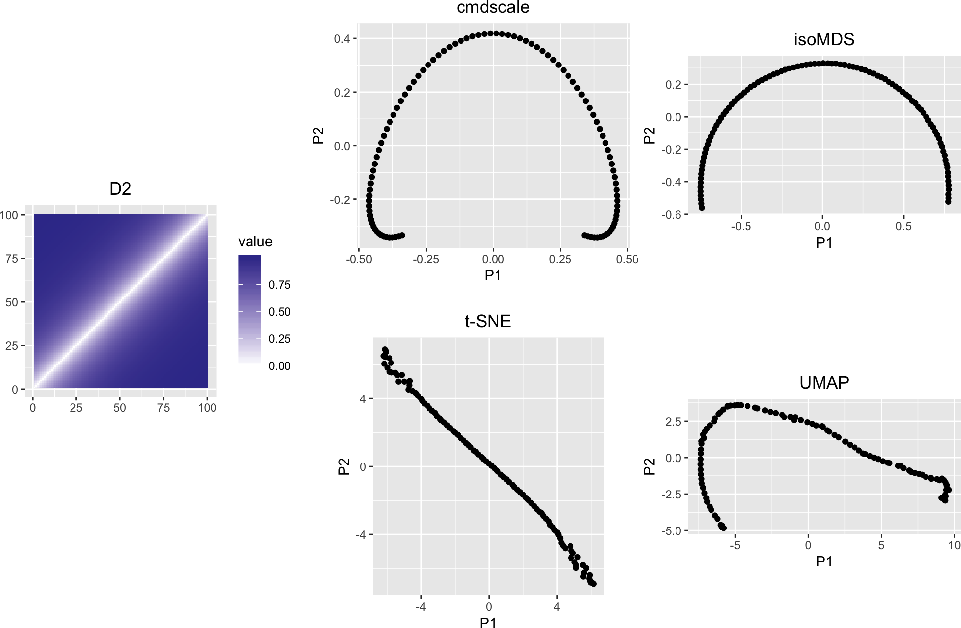

$Like Figure \@ref(fig:diac1), but with a different value of `lambda`, that is, more rapid distance increase away from the diagonal.$

Figure 2: Like Figure 1, but with a different value of lambda, that is, more rapid distance increase away from the diagonal

D3 <- diaconisMatrix(lambda = 20, n = 100)
variousMDSPlots(D3)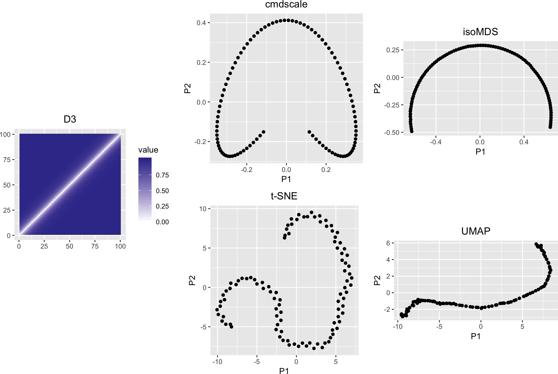

$Like Figures \@ref(fig:diac1) and \@ref(fig:diac2), but with even higher `lambda`.$

Figure 3: Like Figures 1 and 2, but with even higher lambda

The horseshoe becomes even bendier. In some of these plots, the endpoints (1st and $n$-th object) are laid out closer to each other than to the objects in the middle, even though this disrespects the true distances D2, D3.

Let’s look at some of the eigenvectors of the distance matrix D, after double centering. These are used by cmdscale (albeit not directly by the other methods).

eigD <- eigen(multivariance:::double.center(D, normalize = FALSE))
colnames(eigD$vectors) <- paste0("EV", seq_len(ncol(D)))
pairs(eigD$vectors[, 1:5])

Figure 4: Eigenvectors (pairs plot)

ggplot(melt(eigD$vectors[, 1:5], id = "x") %>% mutate(Var2 = factor(Var2)), 
       aes_string(x = "Var1", y = "value", colour = "Var2", group = "Var2")) +
  geom_line(size = sqrt(2)) + 
  scale_colour_manual("Eigenvectors", values = unname(pals::alphabet(5)))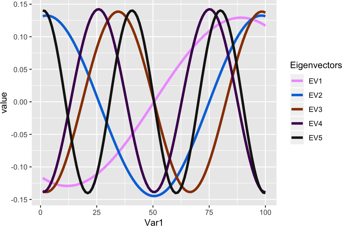

Figure 5: Eigenvectors, scaled to unit length

ev <- eigD$vectors[, 1:5] * 
  matrix(eigD$values[1:5], byrow = TRUE, ncol = 5, nrow = nrow(eigD$vectors))
ggplot(melt(ev, id = "x") %>% mutate(Var2 = factor(Var2)), 
       aes_string(x = "Var1", y = "value", colour = "Var2", group = "Var2")) +
  geom_line(size = sqrt(2)) + 
  scale_colour_manual("Eigenvectors", values = unname(pals::alphabet(5)))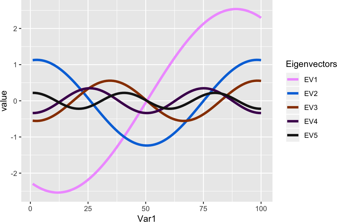

Figure 6: Eigenvectors, scaled by eigenvalue

If we think of the (double centered) matrix $D$ as a discretized version of a differential operator, we see (see Figure 7) that a dominating component is the negative of the second derivative, i.e., $-d^2/dx^2$, and therefore it is not surprising to see eigenfunctions that resemble harmonic functions.

\[ \begin{align} \frac{d^2}{dx^2} f(x) &= \lim_{h\to0} \frac{f(x+h)-2f(x)+f(x-h)}{h^2}\\ -\frac{d^2}{dx^2} f(x) &= k^2 f(x) \Leftrightarrow f(x) \propto e^{ikx} = \cos kx + i \sin kx \end{align} \]

plotMatrixAsImage(multivariance:::double.center(D, normalize = FALSE)) + 
  ggtitle("double centered D")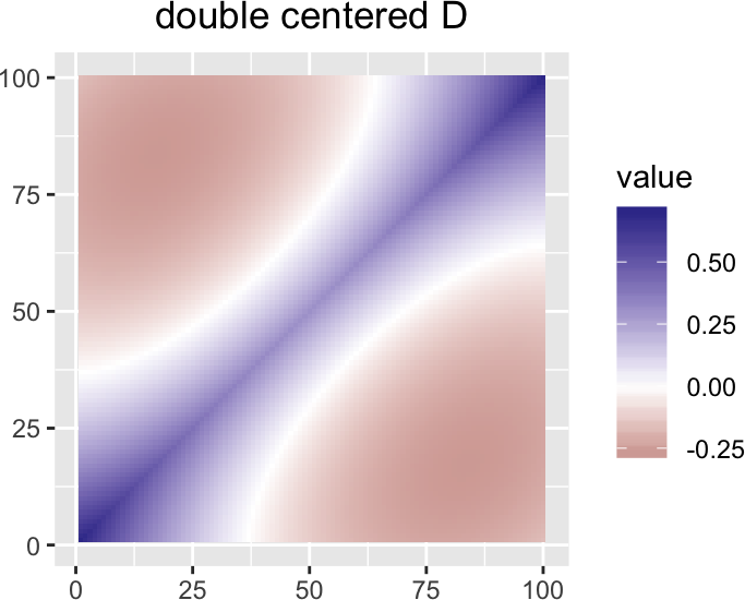

Figure 7: scale(D) as image

2 Points on a straight line

A straight line in ${\mathbb R}^d$ is parameterized by

\[ x = at + b \quad\quad\text{for }t\in{\mathbb R}, \] where $a$ and $b$ are fixed vectors in ${\mathbb R}^n$ (slope and offset). In the code below, we also add some Gaussian noise, with $\sigma=0.5$.

d <- 100   # dimension of the space
n <- 42    # number of points 
t <- seq(0, n, by = 1) %>% matrix(nrow = 1)          # row vector
a <- runif(d) %>% matrix(nrow = d, ncol = 1)         # column vector
b <- runif(d) %>% matrix(nrow = d, ncol = length(t)) # recycle
x <- a %*% t + b
x <- x + matrix(rnorm(prod(dim(x)), sd = 0.5), ncol = ncol(x), nrow = nrow(x))
dm <- as.matrix(dist(t(x)))
variousMDSPlots(dm, perplexity = 10)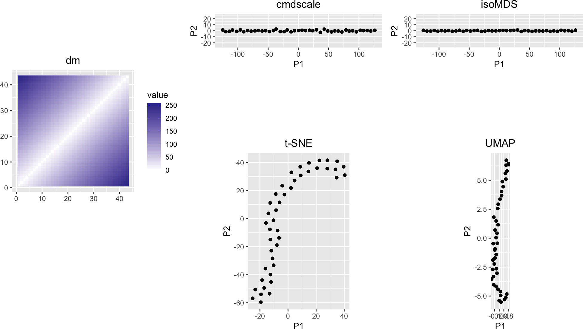

Application of dimension reduction methods to a straight line in feature space. The straight line structure is reasonably preserved, although with some peculiarities in the case ot $t$-SNE.

Figure 8: Application of dimension reduction methods to a straight line in feature space
The straight line structure is reasonably preserved, although with some peculiarities in the case ot $t$-SNE.

2.1 With saturation

Instead of the Euclidean distances, add some saturation (underestimate long distances). For instance, we can take the function $s(x) = 1-e^{-x/x_0}$, for which $s(0)=0$ and $\lim_{x\to\infty}s(x)=1$.

sat <- function(x, x0 = median(x)) { x0 * (1 - exp(-x/x0)) }
ggplot(tibble(x = as.vector(dm),
              y = as.vector(sat(dm))), aes(x = x, y = y)) + 
  geom_line() + xlab("d") + ylab("sat(d)")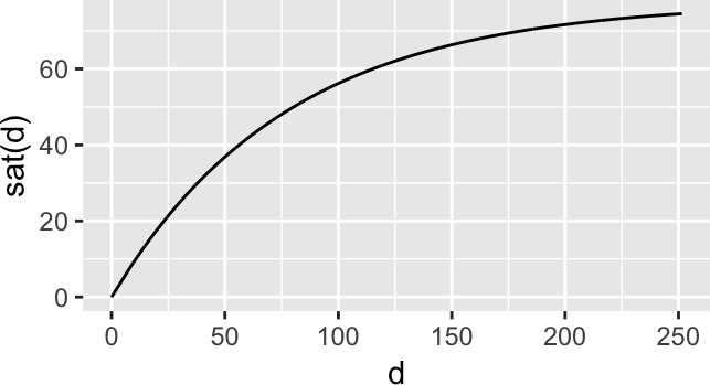

Figure 9: Saturation function

variousMDSPlots(sat(dm), perplexity = 11)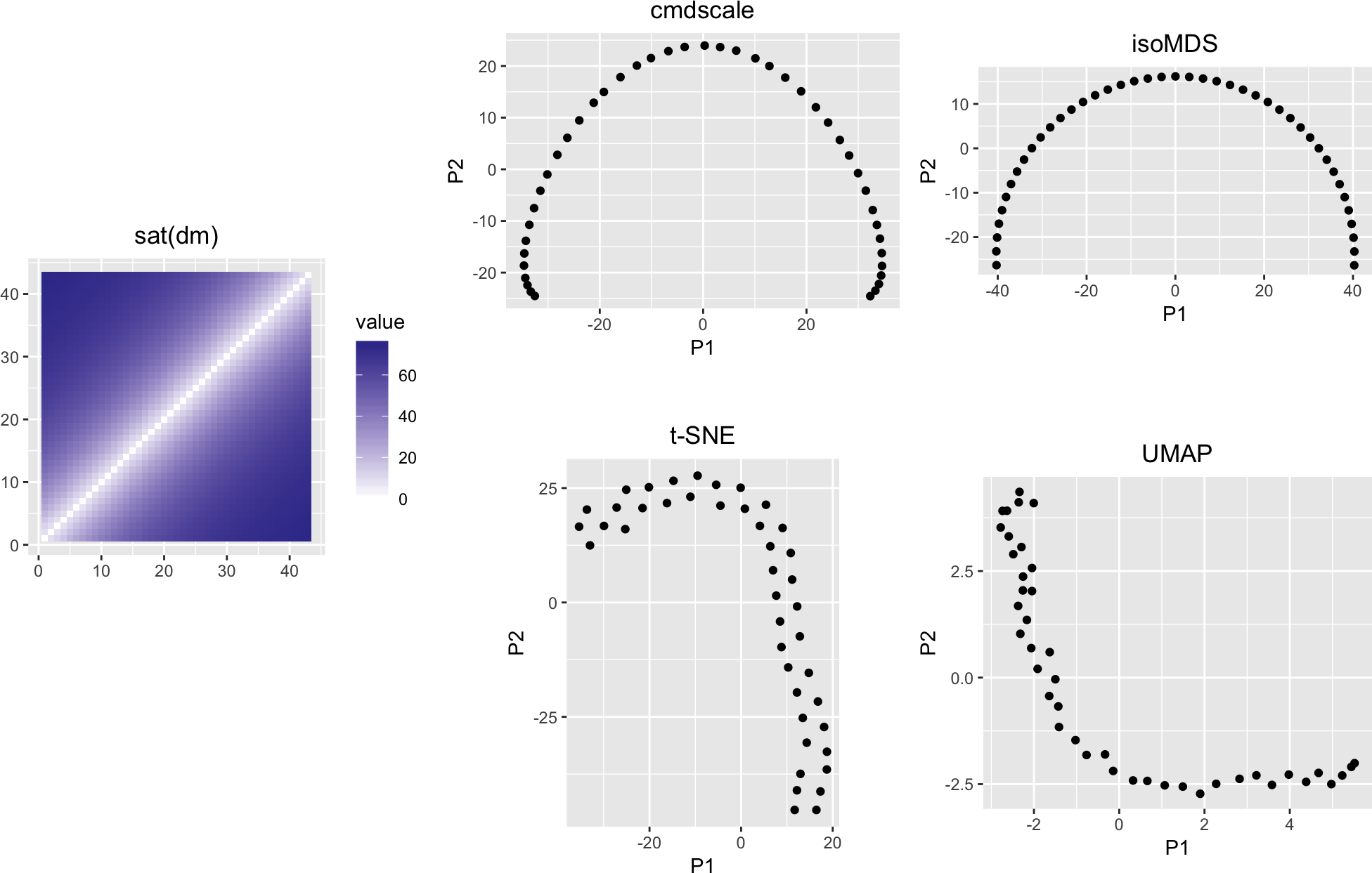

$Like Figure \@ref(fig:straightline1), but with some saturation added (underestimation of long distances).$

Figure 10: Like Figure 8, but with some saturation added (underestimation of long distances)

2.2 With noise

Back to the Euclidean distances, but with noise on the points’ coordinates.

dmnoisy <- as.matrix(dist(t(x + matrix(rnorm(prod(dim(x)), sd = 5), ncol = ncol(x), nrow = nrow(x)))))
variousMDSPlots(dmnoisy, perplexity = 11)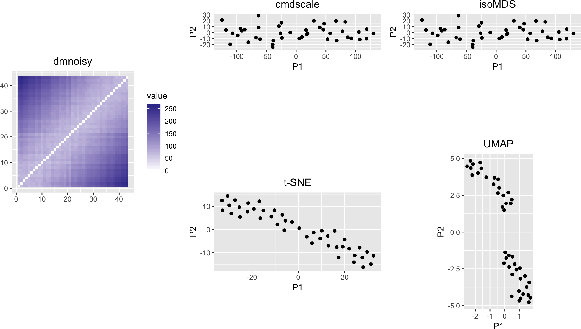

$Like Figure \@ref(fig:straightline1), but with noise.$

Figure 11: Like Figure 8, but with noise

3 Some further curiosities

3.1 2D low pass

In the code below, we create a data matrix of independent, identically distributed random numbers (white.noise), to which we apply a 2D smooothing operator (filter2 from the EBImage package) with bandwidth b. The resulting matrix x has size n times k. (The matrix white.noise has an additional b rows and columns padded to the left, right, top and bottom to avoid having to make choices about how filter2 should deal with the boundaries.)

n <- 100
k <- 150    
b <-  35
white.noise <- matrix(rnorm((k+2*b) * (n+2*b)), nrow = n+2*b, ncol = k+2*b)
smoothened  <- EBImage::filter2(white.noise, EBImage::makeBrush(b))
x <- smoothened[ b+(1:n), b+(1:k) ]

Let’s do a PCA plot of x, using the first two principal components

autoplot(prcomp(x)) + coord_fixed()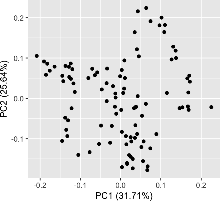

We see an (almost-closed) cycle. If the data were from a single-cell RNA-seq experiment (with, say, n cells and k genes), it could be tempting to see a cellular trajectory that we might think is related to a differentiation process and/or the cell cycle. There are software packages that help fit curves into such plots, which could be interpreted as “pseudo-time”. In many cases, this will be very well (and useful and true) - but in this case we know that the data-generating process had nothing to do with time or some other underlying one-dimensional process or phenomenon. What is going on?

Below, we plot the matrix in false color representation, as well as its covariance matrix.

grid.arrange(plotMatrixAsImage(x), plotMatrixAsImage(cov(x)), ncol = 2)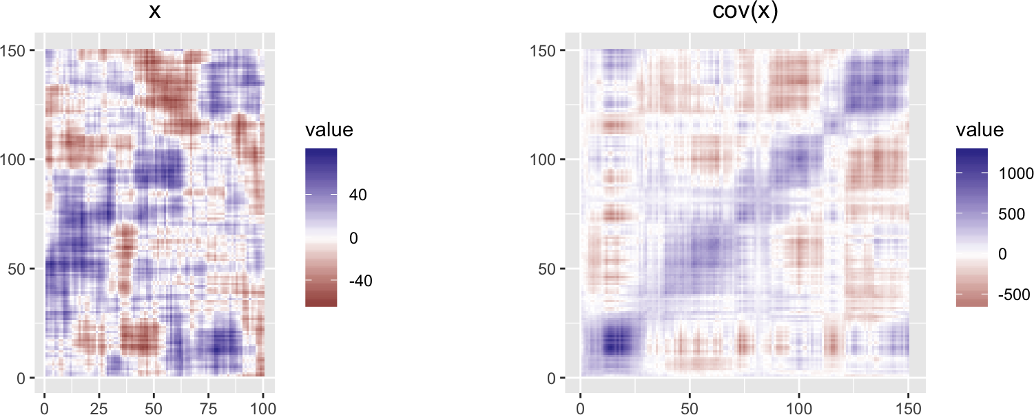

variousMDSPlots(as.matrix(dist(x)))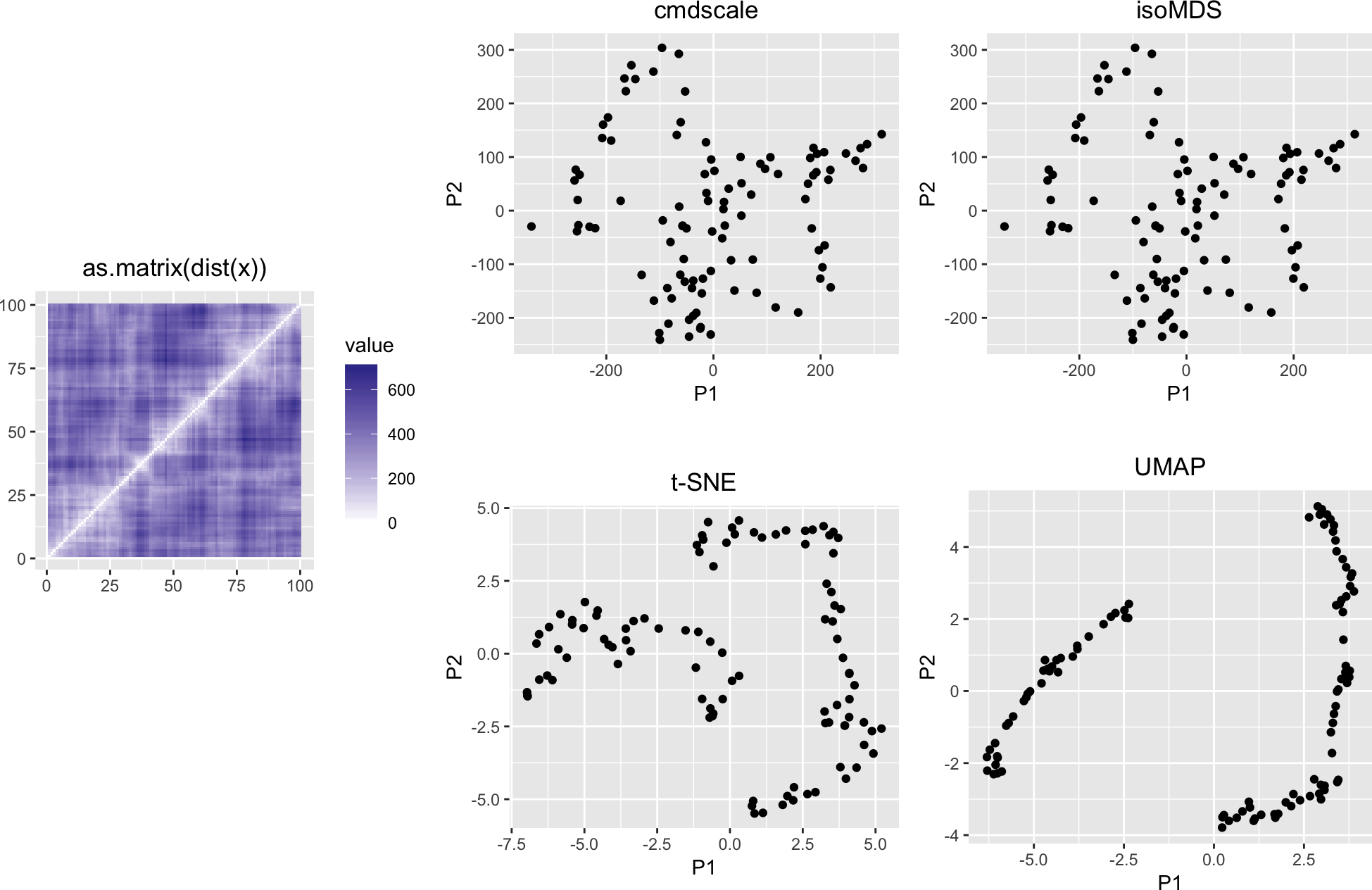

3.2 1D low pass

We can be even more minimalistic with the non-randomness of the input data. In the code below, the k times n matrix rw is filled with the numbers from a random walk (a realisation of 1D Brownian motion).

rw <- matrix(cumsum(rnorm(k*n)), nrow = k, ncol = n)
grid.arrange(plotMatrixAsImage(rw), autoplot(prcomp(rw)) + coord_fixed(), 
             ncol = 2)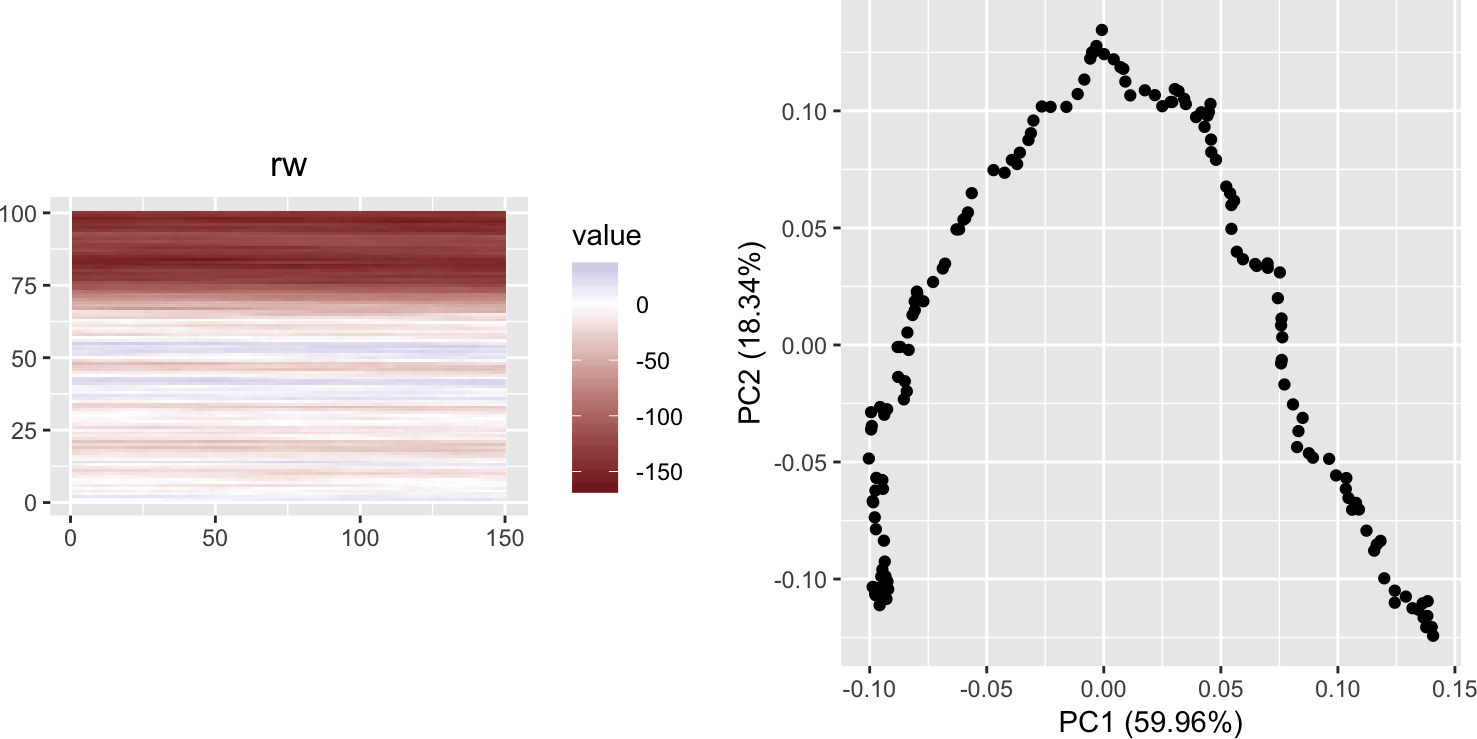

We again see the horseshoe. And interesting patterns in the first five principal components:

pairs(prcomp(rw)$x[, 1:5])

variousMDSPlots(as.matrix(dist(rw)))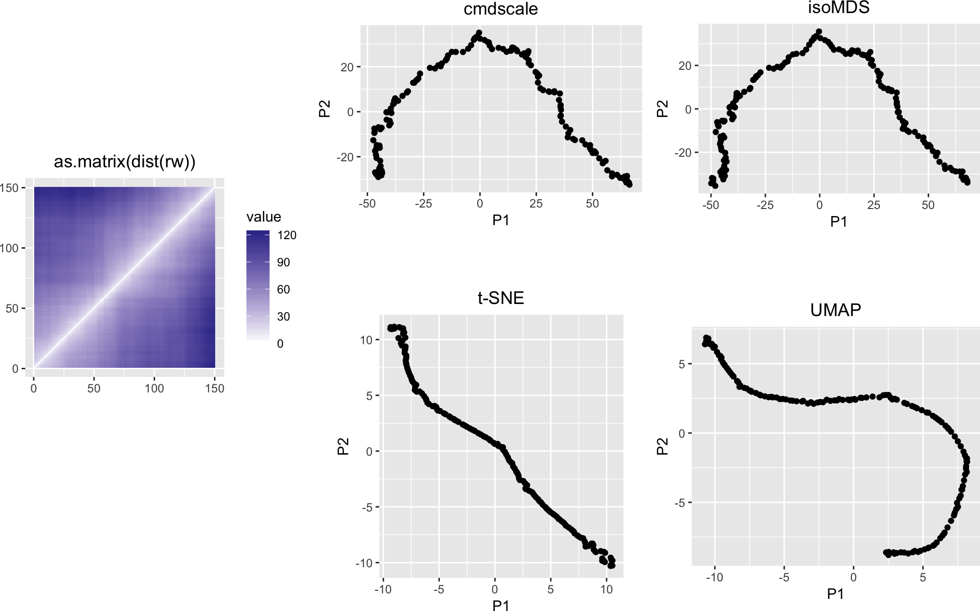

Now, instead of a Brownian motion, let’s just take a series of independent random numbers and subject them to a low-pass filter of window size h (i.e., a running-average smoother).

h  <- 20
rw <- 
  matrix(
    stats::filter(rnorm(k*n + h), rep(1, h))[ h/2 + 1:(n*k) ],
  nrow = k, ncol = n) 
grid.arrange(plotMatrixAsImage(rw), autoplot(prcomp(rw)) + coord_fixed(), 
             ncol = 2)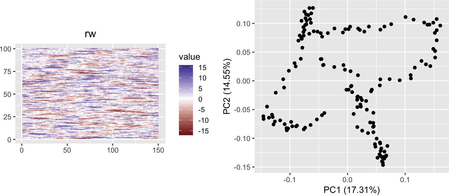

variousMDSPlots(as.matrix(dist(rw)))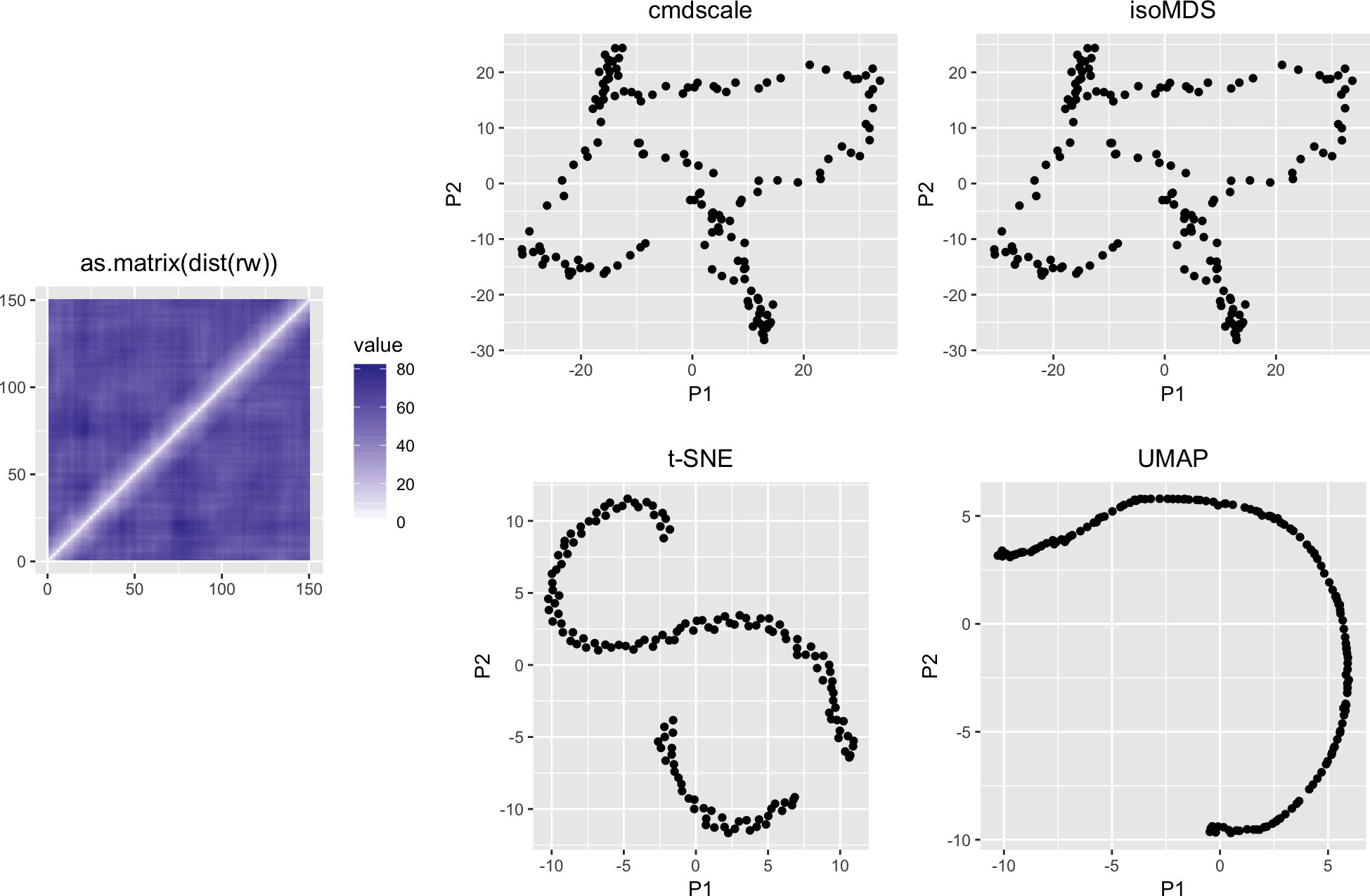

4 Conclusion

Embeddings of high-dimensional data into lower dimensional spaces are useful; but they can also create apparent one-dimensional (“time-like”) patterns that have little to do with the data-generating process. Be aware.

5 Session info

devtools::session_info()

## ─ Session info ────────────────────────────────────────────────────────────
##  setting  value                       
##  version  R version 3.5.3 (2019-03-11)
##  os       macOS Mojave 10.14.4        
##  system   x86_64, darwin15.6.0        
##  ui       X11                         
##  language (EN)                        
##  collate  en_US.UTF-8                 
##  ctype    en_US.UTF-8                 
##  tz       Europe/Berlin               
##  date     2019-04-04                  
## 
## ─ Packages ────────────────────────────────────────────────────────────────
##  package          * version   date       lib source        
##  abind              1.4-5     2016-07-21 [1] CRAN (R 3.5.0)
##  assertthat         0.2.1     2019-03-21 [1] CRAN (R 3.5.3)
##  backports          1.1.3     2018-12-14 [1] CRAN (R 3.5.0)
##  BiocGenerics       0.28.0    2018-10-30 [1] Bioconductor  
##  BiocManager        1.30.4    2018-11-13 [1] CRAN (R 3.5.0)
##  BiocStyle        * 2.10.0    2018-10-30 [1] Bioconductor  
##  bitops             1.0-6     2013-08-17 [1] CRAN (R 3.5.0)
##  bookdown           0.9       2018-12-21 [1] CRAN (R 3.5.0)
##  callr              3.2.0     2019-03-15 [1] CRAN (R 3.5.2)
##  cli                1.1.0     2019-03-19 [1] CRAN (R 3.5.2)
##  codetools          0.2-16    2018-12-24 [1] CRAN (R 3.5.3)
##  colorspace         1.4-1     2019-03-18 [1] CRAN (R 3.5.2)
##  conflicted       * 1.0.2     2019-03-29 [1] CRAN (R 3.5.3)
##  crayon             1.3.4     2017-09-16 [1] CRAN (R 3.5.0)
##  crosstalk          1.0.0     2016-12-21 [1] CRAN (R 3.5.0)
##  desc               1.2.0     2018-05-01 [1] CRAN (R 3.5.0)
##  devtools           2.0.1     2018-10-26 [1] CRAN (R 3.5.1)
##  dichromat          2.0-0     2013-01-24 [1] CRAN (R 3.5.0)
##  digest             0.6.18    2018-10-10 [1] CRAN (R 3.5.0)
##  dplyr            * 0.8.0.1   2019-02-15 [1] CRAN (R 3.5.2)
##  EBImage            4.24.0    2018-10-30 [1] Bioconductor  
##  evaluate           0.13      2019-02-12 [1] CRAN (R 3.5.2)
##  fftwtools          0.9-8     2017-03-25 [1] CRAN (R 3.5.0)
##  fs                 1.2.7     2019-03-19 [1] CRAN (R 3.5.2)
##  ggfortify        * 0.4.6     2019-03-20 [1] CRAN (R 3.5.2)
##  ggplot2          * 3.1.0     2018-10-25 [1] CRAN (R 3.5.0)
##  glue               1.3.1     2019-03-12 [1] CRAN (R 3.5.2)
##  gridExtra        * 2.3       2017-09-09 [1] CRAN (R 3.5.0)
##  gtable             0.3.0     2019-03-25 [1] CRAN (R 3.5.3)
##  highr              0.8       2019-03-20 [1] CRAN (R 3.5.3)
##  htmltools          0.3.6     2017-04-28 [1] CRAN (R 3.5.0)
##  htmlwidgets        1.3       2018-09-30 [1] CRAN (R 3.5.1)
##  httpuv             1.5.0     2019-03-15 [1] CRAN (R 3.5.2)
##  jpeg               0.1-8     2014-01-23 [1] CRAN (R 3.5.0)
##  jsonlite           1.6       2018-12-07 [1] CRAN (R 3.5.0)
##  knitr              1.22      2019-03-08 [1] CRAN (R 3.5.2)
##  labeling           0.3       2014-08-23 [1] CRAN (R 3.5.0)
##  later              0.8.0     2019-02-11 [1] CRAN (R 3.5.2)
##  lattice            0.20-38   2018-11-04 [1] CRAN (R 3.5.3)
##  lazyeval           0.2.2     2019-03-15 [1] CRAN (R 3.5.2)
##  locfit             1.5-9.1   2013-04-20 [1] CRAN (R 3.5.0)
##  magrittr           1.5       2014-11-22 [1] CRAN (R 3.5.0)
##  manipulateWidget   0.10.0    2018-06-11 [1] CRAN (R 3.5.0)
##  mapproj            1.2.6     2018-03-29 [1] CRAN (R 3.5.0)
##  maps               3.3.0     2018-04-03 [1] CRAN (R 3.5.0)
##  MASS               7.3-51.3  2019-03-31 [1] CRAN (R 3.5.3)
##  Matrix             1.2-17    2019-03-22 [1] CRAN (R 3.5.3)
##  memoise            1.1.0     2017-04-21 [1] CRAN (R 3.5.0)
##  mime               0.6       2018-10-05 [1] CRAN (R 3.5.1)
##  miniUI             0.1.1.1   2018-05-18 [1] CRAN (R 3.5.0)
##  multivariance      2.1.0     2019-03-19 [1] CRAN (R 3.5.2)
##  munsell            0.5.0     2018-06-12 [1] CRAN (R 3.5.0)
##  pals               1.5       2018-01-22 [1] CRAN (R 3.5.0)
##  pillar             1.3.1     2018-12-15 [1] CRAN (R 3.5.0)
##  pkgbuild           1.0.3     2019-03-20 [1] CRAN (R 3.5.3)
##  pkgconfig          2.0.2     2018-08-16 [1] CRAN (R 3.5.0)
##  pkgload            1.0.2     2018-10-29 [1] CRAN (R 3.5.0)
##  plyr               1.8.4     2016-06-08 [1] CRAN (R 3.5.0)
##  png                0.1-7     2013-12-03 [1] CRAN (R 3.5.0)
##  prettyunits        1.0.2     2015-07-13 [1] CRAN (R 3.5.0)
##  processx           3.3.0     2019-03-10 [1] CRAN (R 3.5.2)
##  promises           1.0.1     2018-04-13 [1] CRAN (R 3.5.0)
##  ps                 1.3.0     2018-12-21 [1] CRAN (R 3.5.0)
##  purrr              0.3.2     2019-03-15 [1] CRAN (R 3.5.2)
##  R6                 2.4.0     2019-02-14 [1] CRAN (R 3.5.2)
##  Rcpp               1.0.1     2019-03-17 [1] CRAN (R 3.5.2)
##  RCurl              1.95-4.12 2019-03-04 [1] CRAN (R 3.5.2)
##  remotes            2.0.2     2018-10-30 [1] CRAN (R 3.5.0)
##  reshape2         * 1.4.3     2017-12-11 [1] CRAN (R 3.5.0)
##  reticulate         1.11.1    2019-03-06 [1] CRAN (R 3.5.2)
##  rgl                0.100.19  2019-03-12 [1] CRAN (R 3.5.2)
##  rlang              0.3.3     2019-03-29 [1] CRAN (R 3.5.3)
##  rmarkdown          1.12      2019-03-14 [1] CRAN (R 3.5.2)
##  rprojroot          1.3-2     2018-01-03 [1] CRAN (R 3.5.0)
##  RSpectra           0.13-1    2018-05-22 [1] CRAN (R 3.5.0)
##  Rtsne            * 0.15      2018-11-10 [1] CRAN (R 3.5.0)
##  scales             1.0.0     2018-08-09 [1] CRAN (R 3.5.1)
##  sessioninfo        1.1.1     2018-11-05 [1] CRAN (R 3.5.0)
##  shiny              1.2.0     2018-11-02 [1] CRAN (R 3.5.0)
##  stringi            1.4.3     2019-03-12 [1] CRAN (R 3.5.2)
##  stringr            1.4.0     2019-02-10 [1] CRAN (R 3.5.2)
##  testthat           2.0.1     2018-10-13 [1] CRAN (R 3.5.1)
##  tibble             2.1.1     2019-03-16 [1] CRAN (R 3.5.2)
##  tidyr              0.8.3     2019-03-01 [1] CRAN (R 3.5.2)
##  tidyselect         0.2.5     2018-10-11 [1] CRAN (R 3.5.0)
##  tiff               0.1-5     2013-09-04 [1] CRAN (R 3.5.0)
##  umap             * 0.2.0.0   2018-07-25 [1] CRAN (R 3.5.2)
##  usethis            1.4.0     2018-08-14 [1] CRAN (R 3.5.0)
##  webshot            0.5.1     2018-09-28 [1] CRAN (R 3.5.0)
##  withr              2.1.2     2018-03-15 [1] CRAN (R 3.5.0)
##  xfun               0.5       2019-02-20 [1] CRAN (R 3.5.2)
##  xtable             1.8-3     2018-08-29 [1] CRAN (R 3.5.0)
##  yaml               2.2.0     2018-07-25 [1] CRAN (R 3.5.0)
## 
## [1] /Library/Frameworks/R.framework/Versions/3.5/Resources/library

LS0tCnN1YnRpdGxlOiAiU3B1cmlvdXMgc3RydWN0dXJlcyBpbiBsYXRlbnQgc3BhY2UgZGVjb21wb3NpdGlvbiBhbmQgbG93LWRpbWVuc2lvbmFsIGVtYmVkZGluZyBtZXRob2RzIgp0aXRsZTogIsOAIGxhIHJlY2hlcmNoZSBkdSB0ZW1wcyBwZXJkdSIKYXV0aG9yOiAiV29sZmdhbmcgSHViZXIiCm91dHB1dDogCiAgQmlvY1N0eWxlOjpodG1sX2RvY3VtZW50OgogICAgbWF0aGpheDogbG9jYWwKICAgIHNlbGZfY29udGFpbmVkOiBmYWxzZQogICAgdG9jOiB5ZXMKICAgIHRvY19mbG9hdDogdHJ1ZQogICAgY29kZV9kb3dubG9hZDogdHJ1ZQotLS0KCmBgYHtyIGdsb2JhbG9wdGlvbnMsIGluY2x1ZGUgPSBGQUxTRX0Ka25pdHI6Om9wdHNfY2h1bmskc2V0KGNhY2hlID0gVFJVRSwgZGV2ID0gYygicG5nIiwgInBkZiIpLCBtZXNzYWdlID0gRkFMU0UsIHdhcm5pbmcgPSBGQUxTRSkKYGBgCgo8IS0tClRPRE86IAotIFN0YXJ0IHdpdGggbGF0ZW50IHNwYWNlIGRlY29tcG9zaXRpb246IDJELCAxRCBsb3cgcGFzcwotIE1vdmUgdG9ydXMuUm1kIGludG8gaGVyZSwgYWxzbyBhcHBseSBjbWRzY2FsZSB0byBzYW1lLCBhbmQgVU1BUAotLT4KClRoaXMgcG9zdCBkaXNjdXNzZXMgaG93IHlvdSBjYW4gZ2V0IGhvcnNlc2hvZS1sb29raW5nIHBhdHRlcm5zIChzb21ldGltZXMgYWxzbyBjYWxsZWQgY3ljbGljLCBvciBVLSBvciBWLXNoYXBlZCkgaW4gY29tbW9uIGRpbWVuc2lvbiByZWR1Y3Rpb24gbWV0aG9kcywgZnJvbSBkYXRhIHRoYXQgYXJlIGdlbmVyYXRlZCBieSBwcm9jZXNzZXMgdGhhdCBoYXZlIGxpdHRsZSB0byBkbyB3aXRoIGhvcnNlc2hvZXMsIGN5Y2xlcywgVXMgb3IgVnMuCgojIERpYWNvbmlzLCBHb2VsIGFuZCBIb2xtZXMKCkluIHRoZWlyIHBhcGVyICJIb3JzZXNob2VzIGluIG11bHRpZGltZW5zaW9uYWwgc2NhbGluZyBhbmQgbG9jYWwga2VybmVsIG1ldGhvZHMiIGluIFRoZSBBbm5hbHMgb2YgQXBwbGllZCBTdGF0aXN0aWNzICgyMDA4KSwgVm9sLiAyLCBwYWdlIDc3NyAoW0RPSTogMTAuMTIxNC8wOC1BT0FTMTY1XShodHRwOi8vYXJ4aXYub3JnL2Ficy8wODExLjE0NzcpKSwgRGlhY29uaXMsIEdvZWwgYW5kIEhvbG1lcyBsb29rZWQgYXQgc2l0dWF0aW9ucyBpbiB3aGljaCB0aGUgZGlzdGFuY2UgbWF0cml4IG9mIGEgc2V0IG9mIG9iamVjdHMgaXMgY29uY2VudHJhdGVkIGFsb25nIHRoZSBkaWFnb25hbCAoc2VlIEZpZ3VyZSBcQHJlZihmaWc6ZGlhYzEpLCB1cHBlciBsZWZ0IHBhbmVsKS4gVGhleSBzZXQgb3V0IGZyb20gdGhlIGV4YW1wbGUgb2YgdGhlIHZvdGluZyByZWNvcmRzIG9mIHRoZSBtZW1iZXJzIG9mIHRoZSAyMDA1IFVuaXRlZCBTdGF0ZXMgSG91c2Ugb2YgUmVwcmVzZW50YXRpdmVzLiBGcm9tIHRoZXNlIHJlY29yZHMsIHRoZXkgY29tcHV0ZWQgYWxsIHBhaXJ3aXNlIGRpc3RhbmNlcyAob3IgZGlzc2ltaWxhcml0aWVzKSwgYXBwbGllZCBjbGFzc2ljYWwgbXVsdGktZGltZW5zaW9uYWwgc2NhbGluZywgYW5kIG9ic2VydmVkIGEgaG9yc2VzaG9lIHBhdHRlcm4uCgpHZW5lcmFsaXppbmcgdGhpcywgYW5kIGZvbGxvd2luZyB0aGUgaWRlYXMgb2YgRGlhY29uaXMsIEdvZWwgYW5kIEhvbG1lcywgY29uc2lkZXIgYSBzZXQgb2Ygb2JqZWN0cyB3aG9zZSAoZGlzKXNpbWlsYXJpdGllcyBhcmUgZGVzY3JpYmVkIGJ5IHRoZSBtYXRyaXggb2YgcGFpcndpc2UgZGlzdGFuY2VzICREJC4gSW4gcGFydGljdWxhciwgY29uc2lkZXIgdGhlIGlkZWFsaXNlZCBzaXR1YXRpb24gb2YgbWF0cmljZXMgbGlrZSB0aGUgZm9sbG93aW5nIG9uZS4gVGhlIGVsZW1lbnRzIG9mICREJCBhcmUgMCBhbG9uZyB0aGUgZGlhZ29uYWwsIGFuZCB0aGUgdmFsdWVzIGluY3JlYXNlIHdpdGggdGhlIGRpc3RhbmNlIGZyb20gdGhlIGRpYWdvbmFsLCB3aXRoIHNvbWUgcmF0ZSAkXGxhbWJkYV57LTF9JCwgdW50aWwgdGhleSBzYXR1cmF0ZSBhdCBzb21lIG1heGltdW0gdmFsdWUsIHdoaWNoIHcubC5vLmcuIHdlIGNhbiBzZXQgdG8gMToKCjxmb250IHNpemU9KzE+CiQkCkRfe2lqfSA9IDEgLSBlXntcZGlzcGxheXN0eWxlIC1cbGFtYmRhIHwgaS1qIHx9CiQkCjwvZm9udD4Kd2hlcmUgJG4kIGlzIGEgcG9zaXRpdmUgaW50ZWdlciwgJGksaj0xLFxsZG90cyxuJCwgYW5kICREJCBpcyBhbiAkblx0aW1lcyBuJCBtYXRyaXguIAoKYGBge3IgdmFyaW91c1Bsb3RzUGFyLCBlY2hvID0gRkFMU0V9CmZ3aWQgPC0gMTAuNQpmaGd0IDwtIDcKYGBgCgpgYGB7ciBkaWFjMSwgZmlnLndpZHRoID0gZndpZCwgZmlnLmhlaWdodCA9IGZoZ3QsIGZpZy53aWRlID0gVFJVRSwgcmVzdWx0cyA9ICJoaWRlIiwgZmlnLmNhcCA9ICJUaGUgbWF0cml4IEQgYW5kIHZhcmlvdXMgdHlwZXMgb2YgbXVsdGlkaW1lbnNpb25hbCBzY2FsaW5nLiBDbGFzc2ljYWwgKGxpbmVhcikgbXVsdGlkaW1lbnNpb25hbCBzY2FsaW5nLCBgY21kc2NhbGVgLCBhbmQgS3J1c2thbCdzIG5vbi1tZXRyaWMgbnVsdGlkaW1lbnNpb25hbCBzY2FsaW5nLCBgaXNvTURTYCwgaW50cm9kdWNlIGFuIGFwcGFyZW50IGN1cnZhdHVyZSwgb3IgaG9yc2VzaG9lIHNoYXBlLCBldmVuIHRob3VnaCB0aGUgbWF0cml4ICREJCBoYXMgYSBzaW1wbGUgYmFuZC1kaWFnb25hbCBzdHJ1Y3R1cmUuIEFsc28gc2hvd24gYXJlIHQtU05FIGFuZCBVTUFQLiJ9CnNldC5zZWVkKDB4YmVkYWRhKQpsaWJyYXJ5KCJjb25mbGljdGVkIikKbGlicmFyeSgiZHBseXIiKQpsaWJyYXJ5KCJnZ3Bsb3QyIikKbGlicmFyeSgiZ3JpZEV4dHJhIikKbGlicmFyeSgicmVzaGFwZTIiKQpsaWJyYXJ5KCJnZ2ZvcnRpZnkiKQpsaWJyYXJ5KCJSdHNuZSIpCmxpYnJhcnkoInVtYXAiKQoKcGxvdE1hdHJpeEFzSW1hZ2UgPC0gZnVuY3Rpb24oeCkgewogIGdncGxvdChtZWx0KHgpLCBhZXMoeCA9IFZhcjEsIHkgPSBWYXIyLCBmaWxsID0gdmFsdWUpKSArIGdlb21fdGlsZSgpICsgCiAgICBzY2FsZV9maWxsX2dyYWRpZW50MigpICsKICAgIGdndGl0bGUoZGVwYXJzZShzdWJzdGl0dXRlKHgpKSkgKyBjb29yZF9maXhlZCgpICsgeGxhYigiIikgKyB5bGFiKCIiKSArCiAgICB0aGVtZShwbG90LnRpdGxlID0gZWxlbWVudF90ZXh0KGhqdXN0ID0gMC41KSkKfQoKcGxvdE1EUyA8LSBmdW5jdGlvbih4LCB0aXQsIGZsaXB5KSB7CiAgZGF0IDwtIGFzX3RpYmJsZShgY29sbmFtZXM8LWAoeCwgYygiUDEiLCAiUDIiKSkpIAogIGlmICh0aXQgJWluJSBmbGlweSkKICAgIGRhdCA8LSBtdXRhdGUoZGF0LCBQMiA9IC1QMikKICBnZ3Bsb3QoZGF0KSArIAogICAgZ2VvbV9wb2ludChhZXMoeCA9IFAxLCB5ID0gUDIpKSArIGNvb3JkX2ZpeGVkKCkgKyAKICAgIGdndGl0bGUodGl0KSArCiAgICB0aGVtZShwbG90LnRpdGxlID0gZWxlbWVudF90ZXh0KGhqdXN0ID0gMC41KSkgKwogICAgZXhwYW5kX2xpbWl0cyh5ID0gYygtMSwgMSkgKiAwLjIgKiBtYXgoYWJzKGRhdCRQMSkpKQp9Cgp2YXJpb3VzTURTUGxvdHMgPC0gZnVuY3Rpb24oLi4uLCBwZXJwbGV4aXR5ID0gMzAsIGZsaXB5ID0gY2hhcmFjdGVyKDApKSB7IAogIGdyaWQuYXJyYW5nZSgKICAgIHBsb3RNYXRyaXhBc0ltYWdlKC4uLiksIAogICAgcGxvdE1EUyhzdGF0czo6Y21kc2NhbGUoLi4uKSwgImNtZHNjYWxlIiwgZmxpcHkpLAogICAgcGxvdE1EUyhNQVNTOjppc29NRFMoLi4uKSRwb2ludHMsICJpc29NRFMiLCBmbGlweSksCiAgICBwbG90TURTKFJ0c25lKC4uLiwgaXNfZGlzdGFuY2UgPSBUUlVFLCBwZXJwbGV4aXR5ID0gcGVycGxleGl0eSkkWSwgInQtU05FIiwgZmxpcHkpLAogICAgcGxvdE1EUyh1bWFwOjp1bWFwKC4uLiwgaW5wdXQgPSAiZGlzdCIpJGxheW91dCwgIlVNQVAiLCBmbGlweSksCiAgICBsYXlvdXRfbWF0cml4ID0gcmJpbmQoYygxLCAyLCAzKSwgYygxLCA0LCA1KSkKICApCn0KCmRpYWNvbmlzTWF0cml4IDwtIGZ1bmN0aW9uKGxhbWJkYSwgbikKICAxIC0gb3V0ZXIoc2VxKDAsIDEsIGxlbmd0aC5vdXQgPSBuKSwgc2VxKDAsIDEsIGxlbmd0aC5vdXQgPSBuKSwgCiAgICAgICAgRlVOID0gZnVuY3Rpb24oYSwgYikgZXhwKC1sYW1iZGEgKiBhYnMoYS1iKSkpCgpEIDwtIGRpYWNvbmlzTWF0cml4KGxhbWJkYSA9IDIsIG4gPSAxMDApCgp2YXJpb3VzTURTUGxvdHMoRCkKYGBgCgpGb3IgZ29vZCBtZWFzdXJlLCBsZXQgdXMgc2VlIHdoYXQgaGFwcGVucyBpZiB3ZSBpbmNyZWFzZSBgbGFtYmRhYCwgaS5lLiwgc2hvcnRlciByYW5nZSBvZiBkaXN0YW5jZSBpbmNyZWFzZSBhd2F5IGZyb20gdGhlIGRpYWdvbmFsLgoKYGBge3IgZGlhYzIsIGZpZy53aWR0aCA9IGZ3aWQsIGZpZy5oZWlnaHQgPSBmaGd0LCBmaWcud2lkZSA9IFRSVUUsIHJlc3VsdHMgPSAiaGlkZSIsIGZpZy5jYXAgPSAiTGlrZSBGaWd1cmUgXFxAcmVmKGZpZzpkaWFjMSksIGJ1dCB3aXRoIGEgZGlmZmVyZW50IHZhbHVlIG9mICBgbGFtYmRhYCwgdGhhdCBpcywgbW9yZSByYXBpZCBkaXN0YW5jZSBpbmNyZWFzZSBhd2F5IGZyb20gdGhlIGRpYWdvbmFsLiJ9CkQyIDwtIGRpYWNvbmlzTWF0cml4KGxhbWJkYSA9IDYsIG4gPSAxMDApCnZhcmlvdXNNRFNQbG90cyhEMiwgZmxpcHkgPSBjKCJjbWRzY2FsZSIsICJpc29NRFMiKSkKYGBgCmBgYHtyIGRpYWMzLCBmaWcud2lkdGggPSBmd2lkLCBmaWcuaGVpZ2h0ID0gZmhndCwgZmlnLndpZGUgPSBUUlVFLCByZXN1bHRzID0gImhpZGUiLCBmaWcuY2FwID0gIkxpa2UgRmlndXJlcyBcXEByZWYoZmlnOmRpYWMxKSBhbmQgXFxAcmVmKGZpZzpkaWFjMiksIGJ1dCB3aXRoIGV2ZW4gaGlnaGVyIGBsYW1iZGFgLiJ9CkQzIDwtIGRpYWNvbmlzTWF0cml4KGxhbWJkYSA9IDIwLCBuID0gMTAwKQp2YXJpb3VzTURTUGxvdHMoRDMpCmBgYAoKVGhlIGhvcnNlc2hvZSBiZWNvbWVzIGV2ZW4gYmVuZGllci4gSW4gc29tZSBvZiB0aGVzZSBwbG90cywgdGhlIGVuZHBvaW50cyAoMXN0IGFuZCAkbiQtdGggb2JqZWN0KSBhcmUgbGFpZCBvdXQgY2xvc2VyIHRvIGVhY2ggb3RoZXIgdGhhbiB0byB0aGUgb2JqZWN0cyBpbiB0aGUgbWlkZGxlLCBldmVuIHRob3VnaCB0aGlzIGRpc3Jlc3BlY3RzIHRoZSB0cnVlIGRpc3RhbmNlcyBgRDJgLCBgRDNgLgoKTGV0J3MgbG9vayBhdCBzb21lIG9mIHRoZSBlaWdlbnZlY3RvcnMgb2YgdGhlIGRpc3RhbmNlIG1hdHJpeCBgRGAsIGFmdGVyIGRvdWJsZSBjZW50ZXJpbmcuIFRoZXNlIGFyZSB1c2VkIGJ5IGBjbWRzY2FsZWAgKGFsYmVpdCBub3QgZGlyZWN0bHkgYnkgdGhlIG90aGVyIG1ldGhvZHMpLgoKYGBge3IgRGVpZ2VudmVjcGFpcnMsIGZpZy53aWR0aCA9IDYsIGZpZy5oZWlnaHQgPSA2LCBmaWcud2lkZSA9IFRSVUUsIGZpZy5jYXAgPSAiRWlnZW52ZWN0b3JzIChwYWlycyBwbG90KS4ifQplaWdEIDwtIGVpZ2VuKG11bHRpdmFyaWFuY2U6Ojpkb3VibGUuY2VudGVyKEQsIG5vcm1hbGl6ZSA9IEZBTFNFKSkKY29sbmFtZXMoZWlnRCR2ZWN0b3JzKSA8LSBwYXN0ZTAoIkVWIiwgc2VxX2xlbihuY29sKEQpKSkKcGFpcnMoZWlnRCR2ZWN0b3JzWywgMTo1XSkKYGBgCgpgYGB7ciBEZWlnZW52ZWNsaW5lczEsIGZpZy53aWR0aCA9IDYsIGZpZy5oZWlnaHQgPSA0LCBmaWcud2lkZSA9IFRSVUUsIGZpZy5jYXAgPSAiRWlnZW52ZWN0b3JzLCBzY2FsZWQgdG8gdW5pdCBsZW5ndGguIn0KZ2dwbG90KG1lbHQoZWlnRCR2ZWN0b3JzWywgMTo1XSwgaWQgPSAieCIpICU+JSBtdXRhdGUoVmFyMiA9IGZhY3RvcihWYXIyKSksIAogICAgICAgYWVzX3N0cmluZyh4ID0gIlZhcjEiLCB5ID0gInZhbHVlIiwgY29sb3VyID0gIlZhcjIiLCBncm91cCA9ICJWYXIyIikpICsKICBnZW9tX2xpbmUoc2l6ZSA9IHNxcnQoMikpICsgCiAgc2NhbGVfY29sb3VyX21hbnVhbCgiRWlnZW52ZWN0b3JzIiwgdmFsdWVzID0gdW5uYW1lKHBhbHM6OmFscGhhYmV0KDUpKSkKYGBgCgpgYGB7ciBEZWlnZW52ZWNsaW5lczIsIGZpZy53aWR0aCA9IDYsIGZpZy5oZWlnaHQgPSA0LCBmaWcud2lkZSA9IFRSVUUsIGZpZy5jYXAgPSAiRWlnZW52ZWN0b3JzLCBzY2FsZWQgYnkgZWlnZW52YWx1ZS4ifQpldiA8LSBlaWdEJHZlY3RvcnNbLCAxOjVdICogCiAgbWF0cml4KGVpZ0QkdmFsdWVzWzE6NV0sIGJ5cm93ID0gVFJVRSwgbmNvbCA9IDUsIG5yb3cgPSBucm93KGVpZ0QkdmVjdG9ycykpCmdncGxvdChtZWx0KGV2LCBpZCA9ICJ4IikgJT4lIG11dGF0ZShWYXIyID0gZmFjdG9yKFZhcjIpKSwgCiAgICAgICBhZXNfc3RyaW5nKHggPSAiVmFyMSIsIHkgPSAidmFsdWUiLCBjb2xvdXIgPSAiVmFyMiIsIGdyb3VwID0gIlZhcjIiKSkgKwogIGdlb21fbGluZShzaXplID0gc3FydCgyKSkgKyAKICBzY2FsZV9jb2xvdXJfbWFudWFsKCJFaWdlbnZlY3RvcnMiLCB2YWx1ZXMgPSB1bm5hbWUocGFsczo6YWxwaGFiZXQoNSkpKQpgYGAKCklmIHdlIHRoaW5rIG9mIHRoZSAoZG91YmxlIGNlbnRlcmVkKSBtYXRyaXggJEQkIGFzIGEgZGlzY3JldGl6ZWQgdmVyc2lvbiBvZiBhIGRpZmZlcmVudGlhbCBvcGVyYXRvciwgd2Ugc2VlIChzZWUgRmlndXJlIFxAcmVmKGZpZzpzY2FsZURtYXRyaXgpKSB0aGF0IGEgZG9taW5hdGluZyBjb21wb25lbnQgaXMgdGhlIG5lZ2F0aXZlIG9mIHRoZSBzZWNvbmQgZGVyaXZhdGl2ZSwgaS5lLiwgJC1kXjIvZHheMiQsIGFuZCB0aGVyZWZvcmUgaXQgaXMgbm90IHN1cnByaXNpbmcgdG8gc2VlIGVpZ2VuZnVuY3Rpb25zIHRoYXQgcmVzZW1ibGUgaGFybW9uaWMgZnVuY3Rpb25zLgoKJCQKXGJlZ2lue2FsaWdufQpcZnJhY3tkXjJ9e2R4XjJ9IGYoeCkgJj0gXGxpbV97aFx0bzB9IFxmcmFje2YoeCtoKS0yZih4KStmKHgtaCl9e2heMn1cXAotXGZyYWN7ZF4yfXtkeF4yfSBmKHgpICY9IGteMiBmKHgpIFxMZWZ0cmlnaHRhcnJvdyBmKHgpIFxwcm9wdG8gZV57aWt4fSA9IFxjb3Mga3ggKyBpIFxzaW4ga3gKXGVuZHthbGlnbn0KJCQKCgpgYGB7ciBzY2FsZURtYXRyaXgsIGZpZy53aWR0aCA9IDQsIGZpZy5oZWlnaHQgPSA0LCBmaWcud2lkZSA9IFRSVUUsIGZpZy5jYXAgPSAic2NhbGUoRCkgYXMgaW1hZ2UifQpwbG90TWF0cml4QXNJbWFnZShtdWx0aXZhcmlhbmNlOjo6ZG91YmxlLmNlbnRlcihELCBub3JtYWxpemUgPSBGQUxTRSkpICsgCiAgZ2d0aXRsZSgiZG91YmxlIGNlbnRlcmVkIEQiKQpgYGAKCiMgUG9pbnRzIG9uIGEgc3RyYWlnaHQgbGluZQoKQSBzdHJhaWdodCBsaW5lIGluICR7XG1hdGhiYiBSfV5kJCBpcyBwYXJhbWV0ZXJpemVkIGJ5CgokJAogeCA9IGF0ICsgYiAgXHF1YWRccXVhZFx0ZXh0e2ZvciB9dFxpbntcbWF0aGJiIFJ9LAokJAp3aGVyZSAkYSQgYW5kICRiJCBhcmUgZml4ZWQgdmVjdG9ycyBpbiAke1xtYXRoYmIgUn1ebiQgKHNsb3BlIGFuZCBvZmZzZXQpLiBJbiB0aGUgY29kZSBiZWxvdywgd2UgYWxzbyBhZGQgc29tZSBHYXVzc2lhbiBub2lzZSwgd2l0aCAkXHNpZ21hPTAuNSQuCgpgYGB7ciBzdHJhaWdodGxpbmUxLCBmaWcud2lkdGggPSBmd2lkLCBmaWcuaGVpZ2h0ID0gZmhndCwgZmlnLndpZGUgPSBUUlVFLCByZXN1bHRzID0gImhpZGUiLCBmaWcuY2FwID0gIkFwcGxpY2F0aW9uIG9mIGRpbWVuc2lvbiByZWR1Y3Rpb24gbWV0aG9kcyB0byBhIHN0cmFpZ2h0IGxpbmUgaW4gZmVhdHVyZSBzcGFjZS4gVGhlIHN0cmFpZ2h0IGxpbmUgc3RydWN0dXJlIGlzIHJlYXNvbmFibHkgcHJlc2VydmVkLCBhbHRob3VnaCB3aXRoIHNvbWUgcGVjdWxpYXJpdGllcyBpbiB0aGUgY2FzZSBvdCAkdCQtU05FLiJ9CmQgPC0gMTAwICAgIyBkaW1lbnNpb24gb2YgdGhlIHNwYWNlCm4gPC0gNDIgICAgIyBudW1iZXIgb2YgcG9pbnRzIAp0IDwtIHNlcSgwLCBuLCBieSA9IDEpICU+JSBtYXRyaXgobnJvdyA9IDEpICAgICAgICAgICMgcm93IHZlY3RvcgphIDwtIHJ1bmlmKGQpICU+JSBtYXRyaXgobnJvdyA9IGQsIG5jb2wgPSAxKSAgICAgICAgICMgY29sdW1uIHZlY3RvcgpiIDwtIHJ1bmlmKGQpICU+JSBtYXRyaXgobnJvdyA9IGQsIG5jb2wgPSBsZW5ndGgodCkpICMgcmVjeWNsZQp4IDwtIGEgJSolIHQgKyBiCnggPC0geCArIG1hdHJpeChybm9ybShwcm9kKGRpbSh4KSksIHNkID0gMC41KSwgbmNvbCA9IG5jb2woeCksIG5yb3cgPSBucm93KHgpKQpkbSA8LSBhcy5tYXRyaXgoZGlzdCh0KHgpKSkKdmFyaW91c01EU1Bsb3RzKGRtLCBwZXJwbGV4aXR5ID0gMTApCmBgYAoKIyMgV2l0aCBzYXR1cmF0aW9uCgpJbnN0ZWFkIG9mIHRoZSBFdWNsaWRlYW4gZGlzdGFuY2VzLCBhZGQgc29tZSBzYXR1cmF0aW9uICh1bmRlcmVzdGltYXRlIGxvbmcgZGlzdGFuY2VzKS4gCkZvciBpbnN0YW5jZSwgd2UgY2FuIHRha2UgdGhlIGZ1bmN0aW9uICRzKHgpID0gMS1lXnsteC94XzB9JCwgZm9yIHdoaWNoICRzKDApPTAkIGFuZCAkXGxpbV97eFx0b1xpbmZ0eX1zKHgpPTEkLgoKYGBge3Igc2F0dXJhdGlvbmZ1bmN0aW9uLCBmaWcud2lkdGggPSAzLjUsIGZpZy5oZWlnaHQgPSAyLCBmaWcud2lkZSA9IFRSVUUsIHJlc3VsdHMgPSAiaGlkZSIsIGZpZy5jYXAgPSAiU2F0dXJhdGlvbiBmdW5jdGlvbiJ9CnNhdCA8LSBmdW5jdGlvbih4LCB4MCA9IG1lZGlhbih4KSkgeyB4MCAqICgxIC0gZXhwKC14L3gwKSkgfQpnZ3Bsb3QodGliYmxlKHggPSBhcy52ZWN0b3IoZG0pLAogICAgICAgICAgICAgIHkgPSBhcy52ZWN0b3Ioc2F0KGRtKSkpLCBhZXMoeCA9IHgsIHkgPSB5KSkgKyAKICBnZW9tX2xpbmUoKSArIHhsYWIoImQiKSArIHlsYWIoInNhdChkKSIpCiAgICAgICAKYGBgCgpgYGB7ciBzdHJhaWdodGxpbmUyLCBmaWcud2lkdGggPSBmd2lkLCBmaWcuaGVpZ2h0ID0gZmhndCwgZmlnLndpZGUgPSBUUlVFLCByZXN1bHRzID0gImhpZGUiLCBmaWcuY2FwID0gIkxpa2UgRmlndXJlIFxcQHJlZihmaWc6c3RyYWlnaHRsaW5lMSksIGJ1dCB3aXRoIHNvbWUgc2F0dXJhdGlvbiBhZGRlZCAodW5kZXJlc3RpbWF0aW9uIG9mIGxvbmcgZGlzdGFuY2VzKS4ifQp2YXJpb3VzTURTUGxvdHMoc2F0KGRtKSwgcGVycGxleGl0eSA9IDExKQpgYGAKCiMjIFdpdGggbm9pc2UKCkJhY2sgdG8gdGhlIEV1Y2xpZGVhbiBkaXN0YW5jZXMsIGJ1dCB3aXRoIG5vaXNlIG9uIHRoZSBwb2ludHMnIGNvb3JkaW5hdGVzLgoKYGBge3Igc3RyYWlnaHRsaW5lMywgZmlnLndpZHRoID0gZndpZCwgZmlnLmhlaWdodCA9IGZoZ3QsIGZpZy53aWRlID0gVFJVRSwgcmVzdWx0cyA9ICJoaWRlIiwgZmlnLmNhcCA9ICJMaWtlIEZpZ3VyZSBcXEByZWYoZmlnOnN0cmFpZ2h0bGluZTEpLCBidXQgd2l0aCBub2lzZS4ifQpkbW5vaXN5IDwtIGFzLm1hdHJpeChkaXN0KHQoeCArIG1hdHJpeChybm9ybShwcm9kKGRpbSh4KSksIHNkID0gNSksIG5jb2wgPSBuY29sKHgpLCBucm93ID0gbnJvdyh4KSkpKSkKdmFyaW91c01EU1Bsb3RzKGRtbm9pc3ksIHBlcnBsZXhpdHkgPSAxMSkKYGBgCgoKIyBTb21lIGZ1cnRoZXIgY3VyaW9zaXRpZXMKIyMgMkQgbG93IHBhc3MKCkluIHRoZSBjb2RlIGJlbG93LCB3ZSBjcmVhdGUgYSBkYXRhIG1hdHJpeCBvZiBpbmRlcGVuZGVudCwgaWRlbnRpY2FsbHkgZGlzdHJpYnV0ZWQKcmFuZG9tIG51bWJlcnMgKGB3aGl0ZS5ub2lzZWApLCB0byB3aGljaCB3ZSBhcHBseSBhIDJEIHNtb29vdGhpbmcgb3BlcmF0b3IgCihgZmlsdGVyMmAgZnJvbSB0aGUgYEVCSW1hZ2VgIHBhY2thZ2UpIHdpdGggYmFuZHdpZHRoIGBiYC4gClRoZSByZXN1bHRpbmcgbWF0cml4IGB4YCBoYXMgc2l6ZSBgbmAgdGltZXMgYGtgLgooVGhlIG1hdHJpeCBgd2hpdGUubm9pc2VgIGhhcyBhbiBhZGRpdGlvbmFsIGBiYCByb3dzIGFuZCBjb2x1bW5zCnBhZGRlZCB0byB0aGUgbGVmdCwgcmlnaHQsIHRvcCBhbmQgYm90dG9tIHRvIGF2b2lkIGhhdmluZyB0byBtYWtlIGNob2ljZXMgYWJvdXQgaG93IGBmaWx0ZXIyYCAKc2hvdWxkIGRlYWwgd2l0aCB0aGUgYm91bmRhcmllcy4pCiAKYGBge3IgMmRsb3dwYXNzc2V0dXB9Cm4gPC0gMTAwCmsgPC0gMTUwICAgIApiIDwtICAzNQp3aGl0ZS5ub2lzZSA8LSBtYXRyaXgocm5vcm0oKGsrMipiKSAqIChuKzIqYikpLCBucm93ID0gbisyKmIsIG5jb2wgPSBrKzIqYikKc21vb3RoZW5lZCAgPC0gRUJJbWFnZTo6ZmlsdGVyMih3aGl0ZS5ub2lzZSwgRUJJbWFnZTo6bWFrZUJydXNoKGIpKQp4IDwtIHNtb290aGVuZWRbIGIrKDE6biksIGIrKDE6aykgXSAKYGBgCgpMZXQncyBkbyBhIFBDQSBwbG90IG9mIGB4YCwgdXNpbmcgdGhlIGZpcnN0IHR3byBwcmluY2lwYWwgY29tcG9uZW50cwoKYGBge3IgMmRsb3dwYXNzcHJjb21wLCBmaWcud2lkdGggPTQgLCBmaWcuaGVpZ2h0ID0gMy41LCByZXN1bHRzID0gImhpZGUifQphdXRvcGxvdChwcmNvbXAoeCkpICsgY29vcmRfZml4ZWQoKQpgYGAKCldlIHNlZSBhbiAoYWxtb3N0LWNsb3NlZCkgY3ljbGUuIElmIHRoZSBkYXRhIHdlcmUgZnJvbSBhIHNpbmdsZS1jZWxsIFJOQS1zZXEgZXhwZXJpbWVudCAKKHdpdGgsIHNheSwgYG5gIGNlbGxzIGFuZCBga2AgZ2VuZXMpLCAKaXQgY291bGQgYmUgdGVtcHRpbmcgdG8gc2VlIGEgY2VsbHVsYXIgdHJhamVjdG9yeSB0aGF0IHdlIG1pZ2h0IHRoaW5rIGlzIHJlbGF0ZWQgdG8gCmEgZGlmZmVyZW50aWF0aW9uIHByb2Nlc3MgYW5kL29yIHRoZSBjZWxsIGN5Y2xlLiAKVGhlcmUgYXJlIHNvZnR3YXJlIHBhY2thZ2VzIHRoYXQgaGVscCBmaXQgY3VydmVzIGludG8gc3VjaCBwbG90cywgd2hpY2ggY291bGQgYmUgCmludGVycHJldGVkIGFzICJwc2V1ZG8tdGltZSIuCkluIG1hbnkgY2FzZXMsIHRoaXMgd2lsbCBiZSB2ZXJ5IHdlbGwgKGFuZCB1c2VmdWwgYW5kIHRydWUpIC0gYnV0IGluIHRoaXMgY2FzZSB3ZSBrbm93IAp0aGF0IHRoZSBkYXRhLWdlbmVyYXRpbmcgcHJvY2VzcyBoYWQgbm90aGluZyB0byBkbyB3aXRoIHRpbWUgb3Igc29tZSBvdGhlciB1bmRlcmx5aW5nIApvbmUtZGltZW5zaW9uYWwgcHJvY2VzcyBvciBwaGVub21lbm9uLiBXaGF0IGlzIGdvaW5nIG9uPyAKCkJlbG93LCB3ZSBwbG90IHRoZSBtYXRyaXggaW4gZmFsc2UgY29sb3IgcmVwcmVzZW50YXRpb24sIGFzIHdlbGwgYXMgaXRzIGNvdmFyaWFuY2UgbWF0cml4LgoKYGBge3IgMmRsb3dwYXNzbWF0cmljZXMsIGZpZy53aWR0aCA9IDksIGZpZy5oZWlnaHQgPSAzLjUsIHJlc3VsdHMgPSAiaGlkZSJ9CmdyaWQuYXJyYW5nZShwbG90TWF0cml4QXNJbWFnZSh4KSwgcGxvdE1hdHJpeEFzSW1hZ2UoY292KHgpKSwgbmNvbCA9IDIpCmBgYAoKYGBge3IgMmRsb3dwYXNzbWRzLCBmaWcud2lkdGggPSBmd2lkLCBmaWcuaGVpZ2h0ID0gZmhndCwgZmlnLndpZGUgPSBUUlVFLCByZXN1bHRzID0gImhpZGUifQp2YXJpb3VzTURTUGxvdHMoYXMubWF0cml4KGRpc3QoeCkpKQpgYGAKCiMjIDFEIGxvdyBwYXNzCgpXZSBjYW4gYmUgZXZlbiBtb3JlIG1pbmltYWxpc3RpYyB3aXRoIHRoZSBub24tcmFuZG9tbmVzcyBvZiB0aGUgaW5wdXQgZGF0YS4gCkluIHRoZSBjb2RlIGJlbG93LCB0aGUgYGtgIHRpbWVzIGBuYCBtYXRyaXggYHJ3YCBpcyBmaWxsZWQgd2l0aCB0aGUgbnVtYmVycyBmcm9tIAphIHJhbmRvbSB3YWxrIChhIHJlYWxpc2F0aW9uIG9mIDFEIEJyb3duaWFuIG1vdGlvbikuCgpgYGB7ciAxZGxvd3Bhc3NtYXRyaWNlcywgZmlnLndpZHRoID0gOCwgZmlnLmhlaWdodCA9IDQsIGZpZy53aWRlID0gVFJVRSwgd2FybmluZz1GQUxTRX0KcncgPC0gbWF0cml4KGN1bXN1bShybm9ybShrKm4pKSwgbnJvdyA9IGssIG5jb2wgPSBuKQpncmlkLmFycmFuZ2UocGxvdE1hdHJpeEFzSW1hZ2UocncpLCBhdXRvcGxvdChwcmNvbXAocncpKSArIGNvb3JkX2ZpeGVkKCksIAogICAgICAgICAgICAgbmNvbCA9IDIpCmBgYAoKV2UgYWdhaW4gc2VlIHRoZSBob3JzZXNob2UuIEFuZCBpbnRlcmVzdGluZyBwYXR0ZXJucyBpbiB0aGUgZmlyc3QgZml2ZSBwcmluY2lwYWwgY29tcG9uZW50czoKCmBgYHtyIDFkbG93cGFzc3BhaXJzLCBmaWcud2lkdGggPSA2LCBmaWcuaGVpZ2h0ID0gNn0KcGFpcnMocHJjb21wKHJ3KSR4WywgMTo1XSkKYGBgCgpgYGB7ciAxZGxvd3Bhc3NtZHMsIGZpZy53aWR0aCA9IGZ3aWQsIGZpZy5oZWlnaHQgPSBmaGd0LCBmaWcud2lkZSA9IFRSVUUsIHJlc3VsdHMgPSAiaGlkZSIsIG1lc3NhZ2UgPSBGQUxTRSwgd2FybmluZyA9IEZBTFNFfQp2YXJpb3VzTURTUGxvdHMoYXMubWF0cml4KGRpc3QocncpKSkKYGBgCgpOb3csIGluc3RlYWQgb2YgYSBCcm93bmlhbiBtb3Rpb24sIGxldCdzIGp1c3QgdGFrZSBhIHNlcmllcyBvZiBpbmRlcGVuZGVudCByYW5kb20gbnVtYmVycyBhbmQgCnN1YmplY3QgdGhlbSB0byBhIGxvdy1wYXNzIGZpbHRlciBvZiB3aW5kb3cgc2l6ZSBgaGAgKGkuZS4sIGEgcnVubmluZy1hdmVyYWdlIHNtb290aGVyKS4KCmBgYHtyIHJ1bmF2Z21hdHJpY2VzLCBmaWcud2lkdGggPSA4LCBmaWcuaGVpZ2h0ID0gNCwgZmlnLndpZGUgPSBUUlVFLCB3YXJuaW5nID0gRkFMU0V9CmggIDwtIDIwCnJ3IDwtIAogIG1hdHJpeCgKICAgIHN0YXRzOjpmaWx0ZXIocm5vcm0oaypuICsgaCksIHJlcCgxLCBoKSlbIGgvMiArIDE6KG4qaykgXSwKICBucm93ID0gaywgbmNvbCA9IG4pIApncmlkLmFycmFuZ2UocGxvdE1hdHJpeEFzSW1hZ2UocncpLCBhdXRvcGxvdChwcmNvbXAocncpKSArIGNvb3JkX2ZpeGVkKCksIAogICAgICAgICAgICAgbmNvbCA9IDIpCmBgYAoKYGBge3IgcnVuYXZnbWRzLCBmaWcud2lkdGggPSBmd2lkLCBmaWcuaGVpZ2h0ID0gZmhndCwgZmlnLndpZGUgPSBUUlVFLCByZXN1bHRzID0gImhpZGUifQp2YXJpb3VzTURTUGxvdHMoYXMubWF0cml4KGRpc3QocncpKSkKYGBgCgoKIyBDb25jbHVzaW9uCgpFbWJlZGRpbmdzIG9mIGhpZ2gtZGltZW5zaW9uYWwgZGF0YSBpbnRvIGxvd2VyIGRpbWVuc2lvbmFsIHNwYWNlcyBhcmUgdXNlZnVsOyBidXQgdGhleSBjYW4KYWxzbyBjcmVhdGUgYXBwYXJlbnQgb25lLWRpbWVuc2lvbmFsICgidGltZS1saWtlIikgcGF0dGVybnMgdGhhdCBoYXZlIGxpdHRsZSB0byBkbyAKd2l0aCB0aGUgZGF0YS1nZW5lcmF0aW5nIHByb2Nlc3MuIEJlIGF3YXJlLgoKCiMgU2Vzc2lvbiBpbmZvCgpgYGB7ciBzZXNzaW9uSW5mb30KZGV2dG9vbHM6OnNlc3Npb25faW5mbygpCmBgYAo=

À la recherche du temps perdu

Spurious structures in latent space decomposition and low-dimensional embedding methods

4 April 2019