Section 3: Proteomic signatures of trisomy12
Junyan Lu
2021-02-16
Last updated: 2021-05-06
Checks: 5 2
Knit directory: CLLproteomics_publish_revision/analysis/
This reproducible R Markdown analysis was created with workflowr (version 1.6.2). The Checks tab describes the reproducibility checks that were applied when the results were created. The Past versions tab lists the development history.
The R Markdown is untracked by Git. To know which version of the R Markdown file created these results, you’ll want to first commit it to the Git repo. If you’re still working on the analysis, you can ignore this warning. When you’re finished, you can run wflow_publish to commit the R Markdown file and build the HTML.
Great job! The global environment was empty. Objects defined in the global environment can affect the analysis in your R Markdown file in unknown ways. For reproduciblity it’s best to always run the code in an empty environment.
The command set.seed(20200227) was run prior to running the code in the R Markdown file. Setting a seed ensures that any results that rely on randomness, e.g. subsampling or permutations, are reproducible.
Great job! Recording the operating system, R version, and package versions is critical for reproducibility.
- unnamed-chunk-25
- unnamed-chunk-27
- unnamed-chunk-9
To ensure reproducibility of the results, delete the cache directory manuscript_S3_trisomy12_cache and re-run the analysis. To have workflowr automatically delete the cache directory prior to building the file, set delete_cache = TRUE when running wflow_build() or wflow_publish().
Great job! Using relative paths to the files within your workflowr project makes it easier to run your code on other machines.
Great! You are using Git for version control. Tracking code development and connecting the code version to the results is critical for reproducibility.
The results in this page were generated with repository version 3fb50c5. See the Past versions tab to see a history of the changes made to the R Markdown and HTML files.
Note that you need to be careful to ensure that all relevant files for the analysis have been committed to Git prior to generating the results (you can use wflow_publish or wflow_git_commit). workflowr only checks the R Markdown file, but you know if there are other scripts or data files that it depends on. Below is the status of the Git repository when the results were generated:
Ignored files:
    Ignored:    .DS_Store
    Ignored:    .Rhistory
    Ignored:    .Rproj.user/
    Ignored:    analysis/.DS_Store
    Ignored:    analysis/.Rhistory
    Ignored:    analysis/manuscript_S1_Overview_cache/
    Ignored:    analysis/manuscript_S2_genomicAssociation_cache/
    Ignored:    analysis/manuscript_S3_trisomy12_cache/
    Ignored:    code/.DS_Store
    Ignored:    code/.Rhistory
    Ignored:    data/.DS_Store
    Ignored:    output/.DS_Store

Untracked files:
    Untracked:  analysis/.trisomy12_norm.pdf
    Untracked:  analysis/bufferComplexViolin.pdf
    Untracked:  analysis/buffer_Tri12vsTri19.pdf
    Untracked:  analysis/cohortComposition_all.pdf
    Untracked:  analysis/heatmap_tri12_circle.pdf
    Untracked:  analysis/manuscript_S1_Overview.Rmd
    Untracked:  analysis/manuscript_S2_genomicAssociation.Rmd
    Untracked:  analysis/manuscript_S3_trisomy12.Rmd
    Untracked:  analysis/manuscript_S4_trisomy19.Rmd
    Untracked:  analysis/manuscript_S5_IGHV.Rmd
    Untracked:  analysis/manuscript_S6_del11q.Rmd
    Untracked:  analysis/manuscript_S7_SF3B1.Rmd
    Untracked:  analysis/manuscript_S8_drugResponse_Outcomes.Rmd
    Untracked:  analysis/manuscript_S9_STAT2.Rmd
    Untracked:  analysis/plot_PC1_PC2.pdf
    Untracked:  analysis/timsTOF_validate.Rmd
    Untracked:  analysis/tri12_transEnrich.pdf
    Untracked:  analysis/trisomy12_chr_summary.pdf
    Untracked:  code/utils.R
    Untracked:  data/Annotation file March 2021.xlsx
    Untracked:  data/CAS9results.xlsx
    Untracked:  data/CNV_onChrom.RData
    Untracked:  data/ComplexParticipantsPubMedIdentifiers_human.txt
    Untracked:  data/Fig1A.png
    Untracked:  data/IGLV321_SupplementalTables_R2.xlsx
    Untracked:  data/MOFAout.RData
    Untracked:  data/MOFAout_atLeast3.RData
    Untracked:  data/STATexprPCR.xlsx
    Untracked:  data/Western_blot_results_20210309_short.csv
    Untracked:  data/Western_blot_results_separate_blots.xlsx
    Untracked:  data/allComplexes.txt
    Untracked:  data/ddsrna_enc.RData
    Untracked:  data/exprCNV_enc.RData
    Untracked:  data/geneAnno.RData
    Untracked:  data/gmts/
    Untracked:  data/ic50.RData
    Untracked:  data/mofaIn.RData
    Untracked:  data/mofaIn_atLeast3.RData
    Untracked:  data/patMeta_enc.RData
    Untracked:  data/pepCLL_lumos_enc.RData
    Untracked:  data/protMOFA.RData
    Untracked:  data/proteins_in_complexes
    Untracked:  data/proteomic_LUMOS_2pep_enc.RData
    Untracked:  data/proteomic_explore_enc.RData
    Untracked:  data/proteomic_independent_all_enc.RData
    Untracked:  data/proteomic_independent_enc.RData
    Untracked:  data/proteomic_timsTOF_enc.RData
    Untracked:  data/screenData_enc.RData
    Untracked:  data/setToPathway.txt
    Untracked:  data/survival_enc.RData
    Untracked:  output/MSH6_splicing.svg
    Untracked:  output/SUGP1_splicing.svg
    Untracked:  output/deResList.RData
    Untracked:  output/deResListBatch2.RData
    Untracked:  output/deResListRNA.RData
    Untracked:  output/deResListRNA_allGene.RData
    Untracked:  output/deResList_WBC.RData
    Untracked:  output/deResList_batch1.RData
    Untracked:  output/deResList_batch3.RData
    Untracked:  output/deResList_independent.RData
    Untracked:  output/deResList_timsTOF.RData
    Untracked:  output/dxdCLL.RData
    Untracked:  output/dxdCLL2.RData
    Untracked:  output/exprCNV.RData
    Untracked:  output/geneAnno.RData
    Untracked:  output/int_pairs.csv
    Untracked:  output/lassoResults_CPS.RData
    Untracked:  output/resOutcome_batch1.RData
    Untracked:  output/resOutcome_batch13.RData
    Untracked:  output/resOutcome_batch2.RData
    Untracked:  output/resOutcome_batch3.RData

Unstaged changes:
    Modified:   analysis/_site.yml
    Deleted:    analysis/analysisSF3B1.Rmd
    Deleted:    analysis/comparePlatforms.Rmd
    Deleted:    analysis/compareProteomicsRNAseq.Rmd
    Deleted:    analysis/correlateCLLPD.Rmd
    Deleted:    analysis/correlateGenomic.Rmd
    Deleted:    analysis/correlateGenomic_removePC.Rmd
    Deleted:    analysis/correlateMIR.Rmd
    Deleted:    analysis/correlateMethylationCluster.Rmd
    Modified:   analysis/index.Rmd
    Deleted:    analysis/predictOutcome.Rmd
    Deleted:    analysis/processProteomics_LUMOS.Rmd
    Deleted:    analysis/processProteomics_timsTOF.Rmd
    Deleted:    analysis/qualityControl_LUMOS.Rmd
    Deleted:    analysis/qualityControl_timsTOF.Rmd
Note that any generated files, e.g. HTML, png, CSS, etc., are not included in this status report because it is ok for generated content to have uncommitted changes.
There are no past versions. Publish this analysis with wflow_publish() to start tracking its development.
#Load packages and datasets
Overview of differentially expressed proteins realted to trisomy12
A table of associations with 5% FDR
resList <- filter(resList, Gene == "trisomy12") %>%
  #mutate(adj.P.Val = adj.P.global) %>% #use global corrected P-value
  mutate(Chr = rowData(protCLL[id,])$chromosome_name)
resList %>% filter(adj.P.Val <= 0.05) %>%
  select(name, Chr,logFC, P.Value, adj.P.Val) %>%
  mutate_if(is.numeric, formatC, digits=2) %>%
  DT::datatable()
Heatmap of differentially expressed proteins
proList <- filter(resList, !is.na(name), adj.P.Val < 0.01) %>% distinct(name, .keep_all = TRUE) %>% pull(id)
plotMat <- assays(protCLL)[["QRILC_combat"]][proList,]
rownames(plotMat) <- rowData(protCLL[proList,])$hgnc_symbol

colAnno <- filter(patMeta, Patient.ID %in% colnames(protCLL)) %>%
  select(Patient.ID, trisomy12, IGHV.status) %>%
  data.frame() %>% column_to_rownames("Patient.ID")
colAnno$trisomy12 <- ifelse(colAnno$trisomy12 %in% 1, "yes","no")

rowAnno <- rowData(protCLL)[proList,c("chromosome_name","hgnc_symbol"),drop=FALSE] %>%
  data.frame(stringsAsFactors = FALSE) %>%
  mutate(onChr12 = ifelse(chromosome_name == "12","yes","no")) %>%
  select(hgnc_symbol, onChr12) %>% data.frame() %>% remove_rownames() %>% column_to_rownames("hgnc_symbol")

plotMat <- jyluMisc::mscale(plotMat, censor = 5)

annoCol <- list(trisomy12 = c(yes = "black",no = "grey80"),
                IGHV.status = c(M = colList[4], U = colList[3]),
                onChr12 = c(yes = colList[1],no = "white"))

pheatmap::pheatmap(plotMat, annotation_col = colAnno, scale = "none",
                   annotation_row = rowAnno,
                   clustering_method = "complete", clustering_distance_cols = "euclidean",
                   color = colorRampPalette(c(colList[2],"white",colList[1]))(100),
                   breaks = seq(-5,5, length.out = 101), annotation_colors = annoCol,
                   show_rownames = FALSE, show_colnames = FALSE,
                   treeheight_row = 0)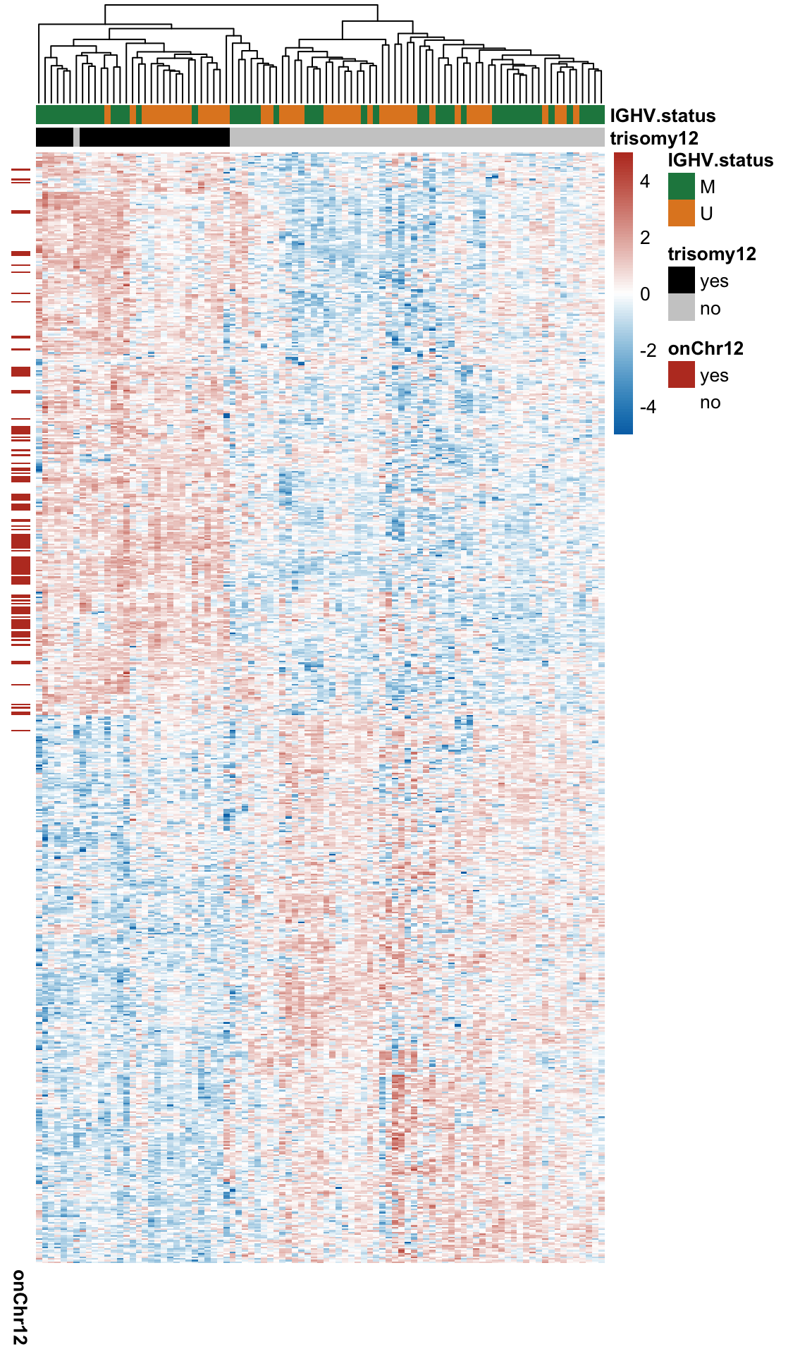
Summary of the chromosome distribution of genes that encode those DE proteins
plotTab <- filter(resList, adj.P.Val <=0.05) %>% mutate(change = ifelse(logFC>0,"Up regulated","Down regulated"),
                              chromosome = ifelse(Chr %in% "12","chr12","other")) %>%
  group_by(change, chromosome) %>% summarise(n = length(id))

sigNumPlot <- ggplot(plotTab, aes(x=change, y=n, fill = chromosome)) +
  geom_bar(stat = "identity", width = 0.8,
           position = position_dodge2(width = 6),
           col = "black") +
  geom_text(aes(label=n),
            position = position_dodge(width = 0.9),
            size=4, hjust=-0.1)  +
  scale_fill_manual(name = "", labels = c("chr12","other"), values = colList) +
  coord_flip(ylim = c(0,700), expand = FALSE) + xlab("") + ylab("Number of associations (5% FDR)") + theme_half +
  theme(legend.text = element_text(size=12))
sigNumPlot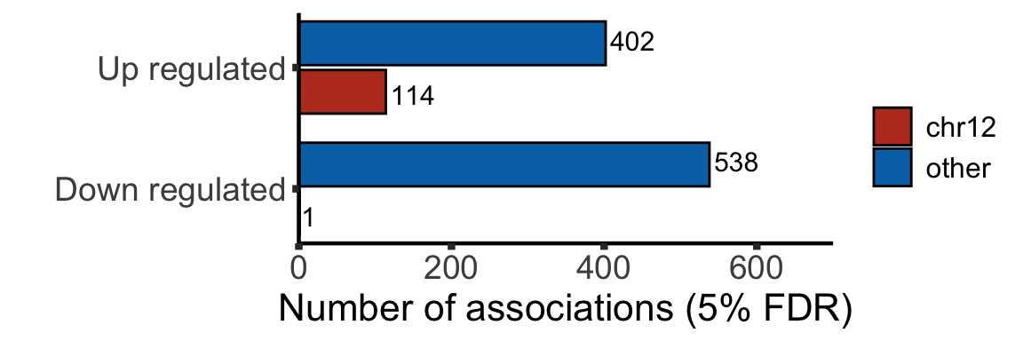
Volcano plot for differentially expressed proteins.
plotTab <- resList
nameList <- c("PTPN11", "BCL10", "SMAD2", "PYCARD", "STAT2", "CD72")
tri12Vocano <- plotVolcano(plotTab, fdrCut =0.05, x_lab=bquote("log"[2]*"(fold change)"), posCol = colList[1], negCol = colList[2],
plotTitle = "trisomy12 (present versus absent)", ifLabel = TRUE, labelList = nameList)
tri12Vocano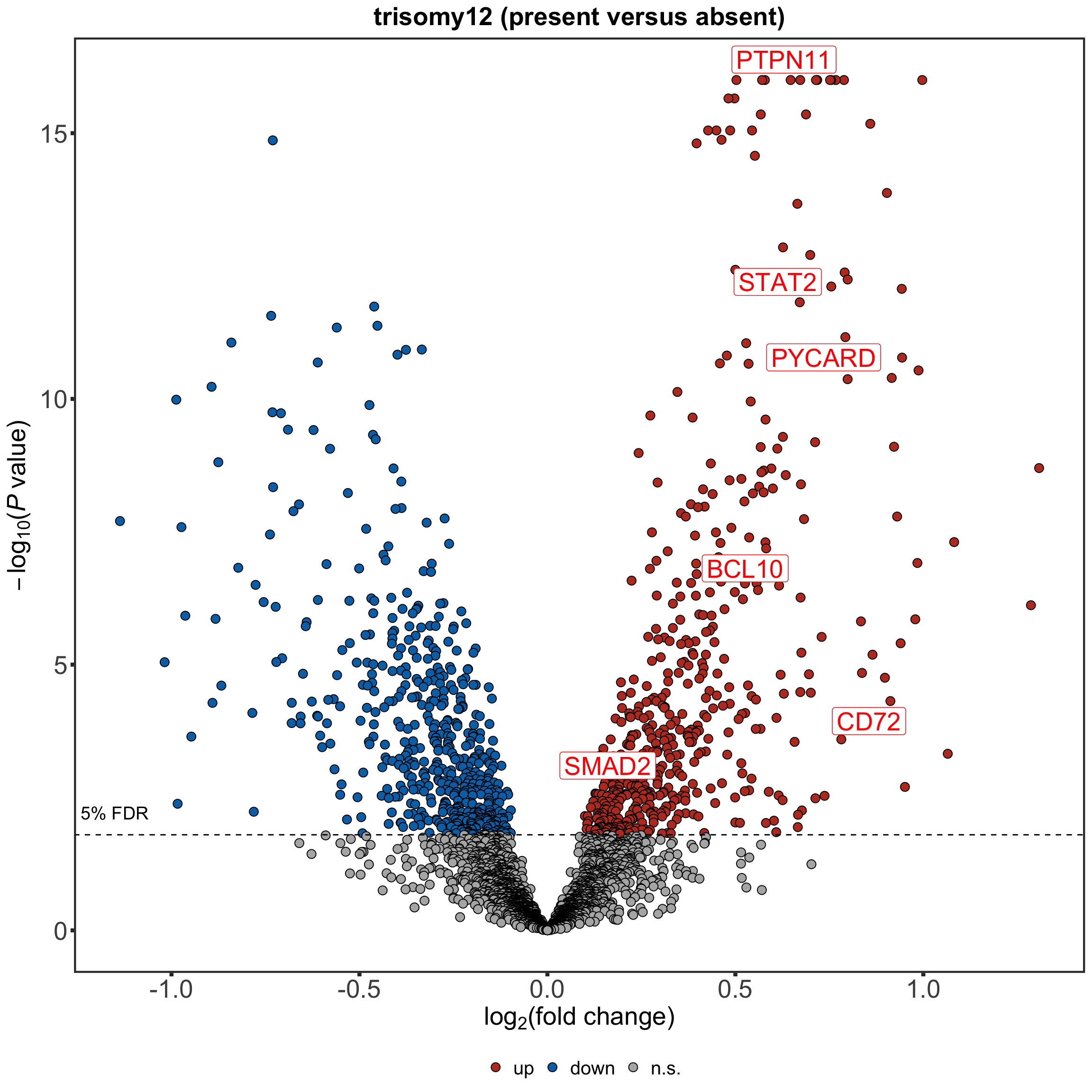 The proteins discussed in the manuscript are labelled.
Boxplot plot of selected genes
protTab <- sumToTidy(protCLL, rowID = "uniprotID", colID = "patID") %>%
  mutate(count = count_combat)
plotTab <- protTab %>% filter(hgnc_symbol %in% nameList) %>%
  mutate(trisomy12 = patMeta[match(patID, patMeta$Patient.ID),]$trisomy12) %>%
  mutate(status = ifelse(trisomy12 %in% 1,"trisomy12","other"),
         name = hgnc_symbol) %>%
  mutate(status = factor(status, levels = c("other","trisomy12")))
pList <- plotBox(plotTab, pValTabel = resList, y_lab = "Protein expression")
protBoxplot <- cowplot::plot_grid(plotlist= pList, ncol=3)
protBoxplot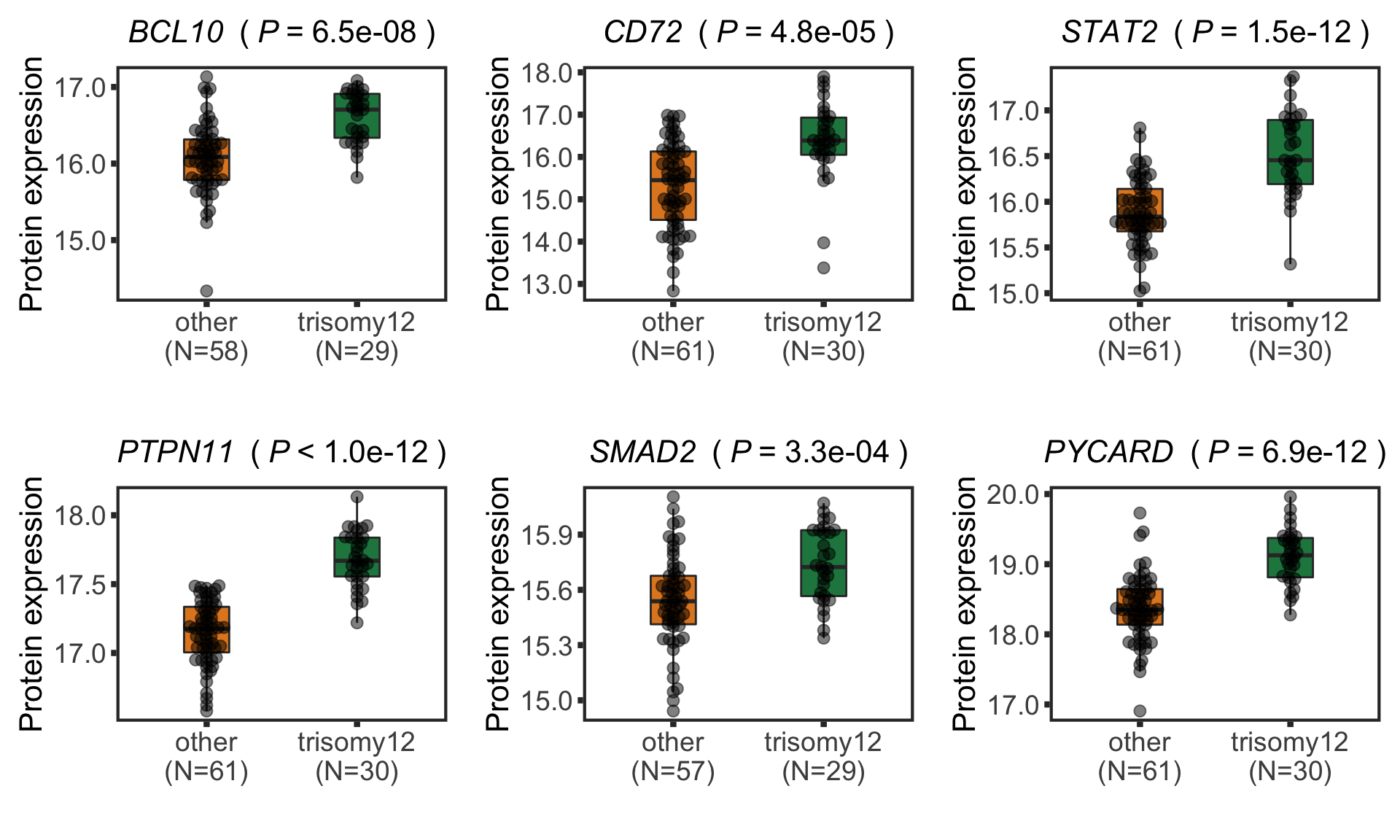
#ggsave("trisomy12_selected_protein.pdf", height = 6, width = 10)Gene set enrichment analysis to explore the pathway changes related to trisomy12
For all differentially expressed proteins
Barplot of enriched pathways using Hallmark gene set
gmts = list(H= "../data/gmts/h.all.v7.3.symbols.gmt",
            KEGG = "../data/gmts/c2.cp.kegg.v7.3.symbols.gmt",
            combine = "../data/gmts/hallmark_kegg_combine.gmt")
inputTab <- resList %>% filter(adj.P.Val < 0.05, Gene == "trisomy12") %>%
  mutate(name = rowData(protCLL[id,])$hgnc_symbol) %>% filter(!is.na(name)) %>%
  distinct(name, .keep_all = TRUE) %>%
  select(name, t) %>% data.frame() %>% column_to_rownames("name")
enRes <- list()
enRes[["Cancer Hallmark gene sets"]] <- runGSEA(inputTab, gmts$H, "page")

tri12Enrich <- plotEnrichmentBar(enRes[[1]], pCut =0.05, ifFDR= TRUE, setName = "",
                       title = names(enRes)[1], removePrefix = "HALLMARK_", insideLegend=TRUE, setMap = setMap) +
  theme(legend.position = "none")
tri12Enrich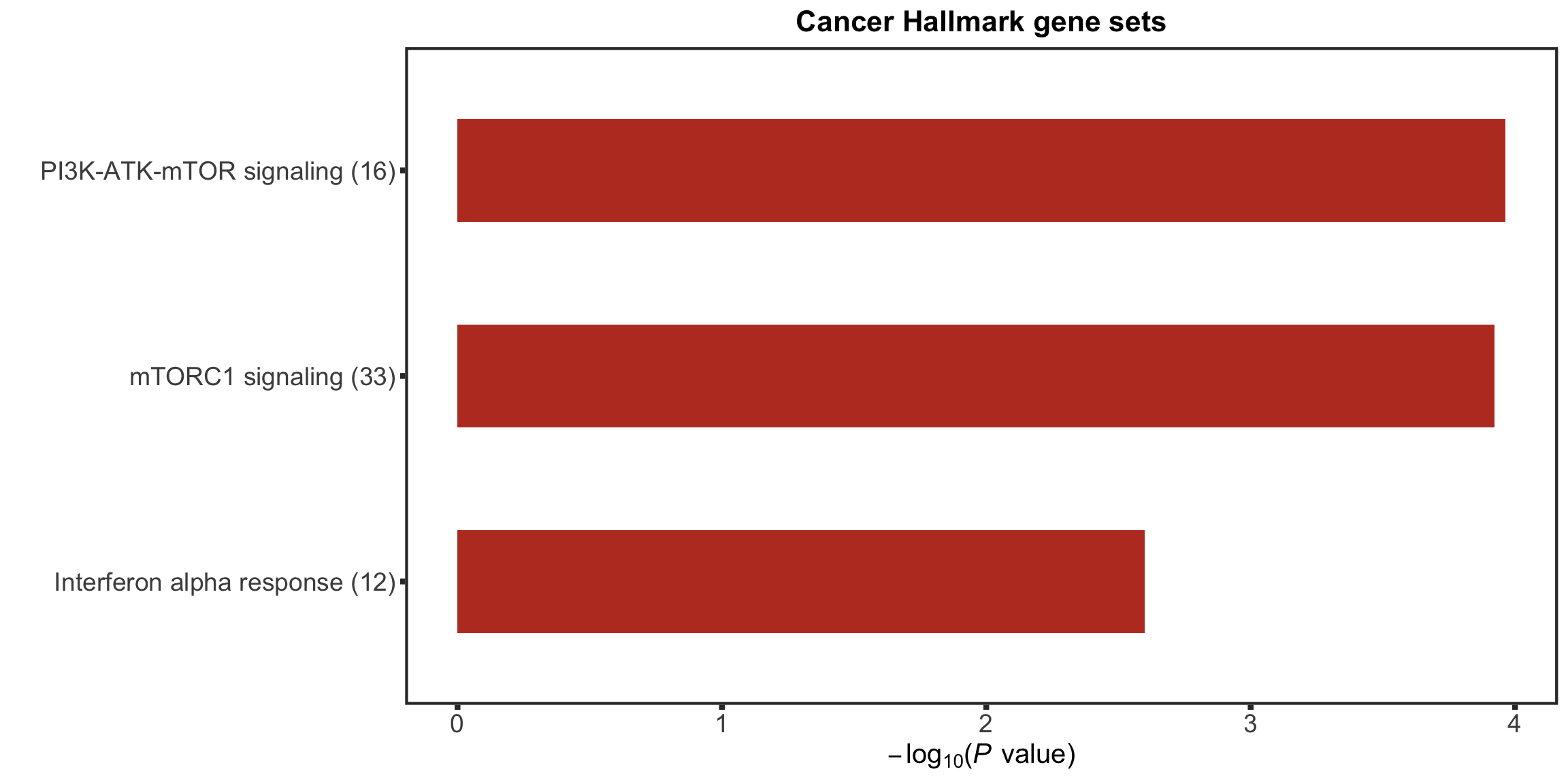
Barplot of enriched pathways using KEGG gene set
inputTab <- resList %>% filter(adj.P.Val < 0.05, Gene == "trisomy12") %>%
  mutate(name = rowData(protCLL[id,])$hgnc_symbol) %>% filter(!is.na(name)) %>%
  distinct(name, .keep_all = TRUE) %>%
  select(name, t) %>% data.frame() %>% column_to_rownames("name")
enRes <- list()
enRes[["KEGG gene sets"]] <- runGSEA(inputTab, gmts$KEGG, "page")

tri12EnrichKEGG <- plotEnrichmentBar(enRes[[1]], pCut =0.05, ifFDR= TRUE, setName =  "",
                       title = names(enRes)[1], removePrefix = "KEGG_", insideLegend=TRUE, setMap = setMap) +
  theme(legend.position = c(0.8,0.2))
For DE proteins encoded by genes on chromosome 12 (cis-effect)
We will use Fisher test to identify geneset that are over-rerepresented.
All protein coding genes in the genome will be used as background
#using all quantified proteins
rnaAll <- dds[rowData(dds)$biotype %in% "protein_coding" & !rowData(dds)$symbol %in% c("",NA),] #all protein coding gene as background
backList <- rowData(rnaAll)$symbol
resListTri12 <- mutate(resList, chr = rowData(protCLL[id,])$chromosome_name)
Enrichment results
protList <- filter(resListTri12, adj.P.Val < 0.05, t>0, chr == "12")$name

enRes <- runFisher(protList, backList, gmts$combine, pCut =0.05, ifFDR = TRUE,removePrefix = "KEGG_|HALLMARK_",
                   plotTitle = "trisomy12 cis-effect", insideLegend = TRUE,
                   setName = "", setMap = setMap, topN=5)
cisComEnrich <- enRes$enrichPlot + theme(plot.margin = margin(1,3,1,1, unit = "cm"))
cisComEnrich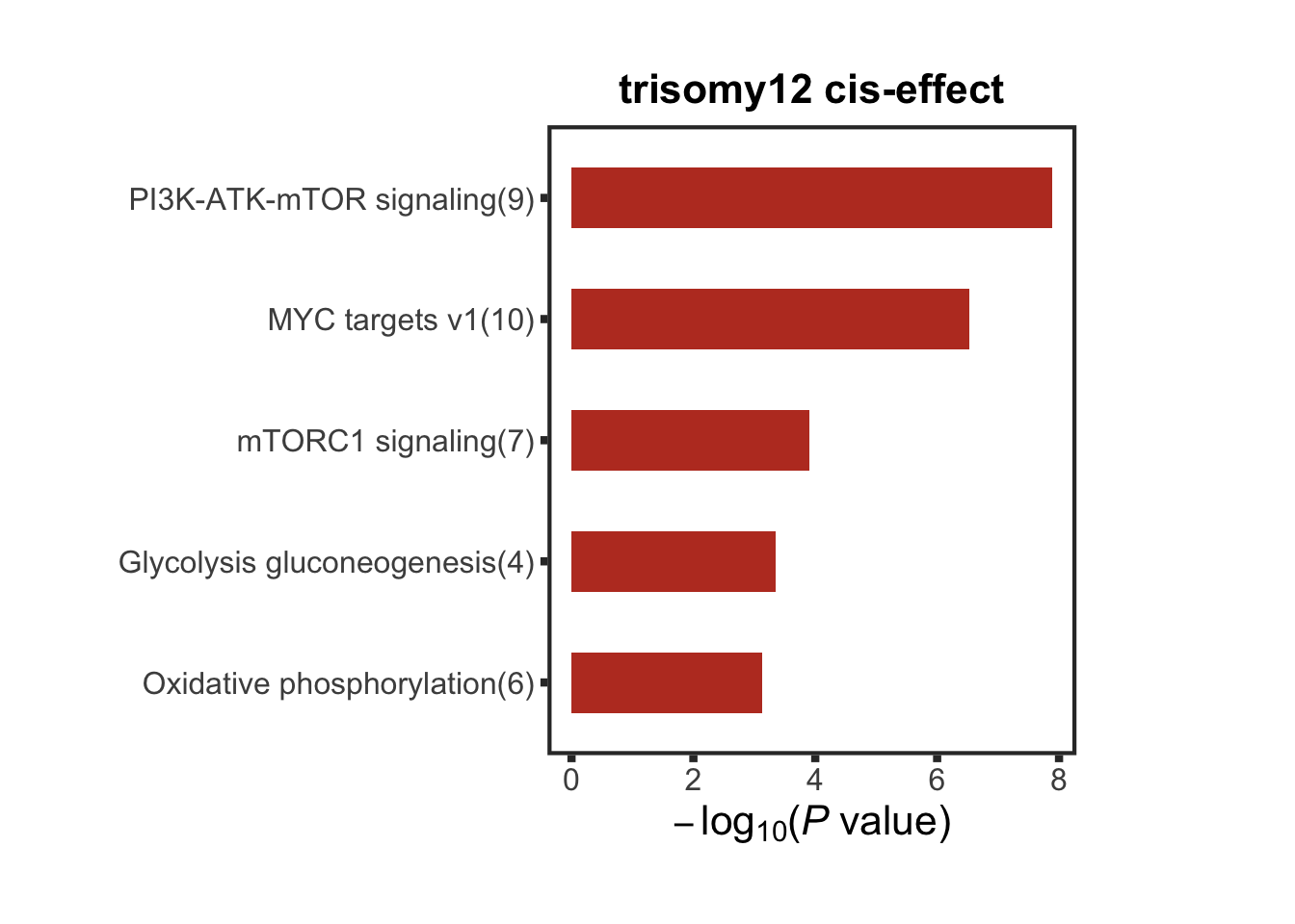
#ggsave("tri12_cisEnrich.pdf", height = 5, width = 7)For proteins not on chr12 (trans-effect)
protList <- filter(resListTri12, adj.P.Val < 0.05, t>0, chr != "12")$name

enRes <- runFisher(protList, backList, gmts$combine, pCut =0.05, ifFDR = TRUE,removePrefix = "KEGG_|HALLMARK_",
                   plotTitle = "trisomy12 trans-effect", insideLegend = TRUE,
                   setName = "", setMap = setMap, topN=5)
transComEnrich <- enRes$enrichPlot + theme(plot.margin = margin(1,3,1,1, unit = "cm"))
transComEnrich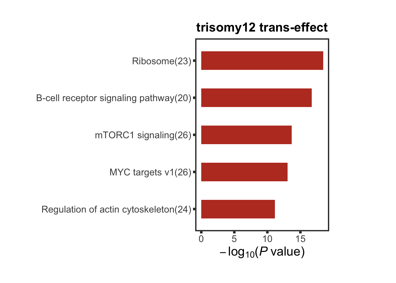
#ggsave("tri12_transEnrich.pdf", height = 5, width = 7)Heatmaps of protein expression in enriched pathways
resList.sig <- filter(resList, !is.na(name), adj.P.Val < 0.05, t>0) %>% distinct(name, .keep_all = TRUE)
upRNAlist <- filter(resListRNA, Gene == "trisomy12") %>% filter(t>0, adj.P.Val <= 0.05) %>% pull(name)
plotMat <- assays(protCLL)[["QRILC_combat"]][resList.sig$id,]
rownames(plotMat) <- rowData(protCLL[rownames(plotMat),])$hgnc_symbol
colAnno <- filter(patMeta, Patient.ID %in% colnames(protCLL)) %>%
  select(Patient.ID, trisomy12) %>%
  data.frame() %>% column_to_rownames("Patient.ID")
colAnno$trisomy12 <- ifelse(colAnno$trisomy12 %in% 1, "yes","no")

rowAnno <- rowData(protCLL)[resList.sig$id,c("chromosome_name","hgnc_symbol"),drop=FALSE] %>%
  data.frame(stringsAsFactors = FALSE) %>%
  mutate(`on Chr12` = ifelse(chromosome_name == "12","yes","no")) %>%
  mutate(`RNA up-regulated` = ifelse(hgnc_symbol %in% upRNAlist,"yes","no")) %>%
  select(hgnc_symbol, `on Chr12`, `RNA up-regulated`) %>% remove_rownames() %>% column_to_rownames("hgnc_symbol")

plotMat <- jyluMisc::mscale(plotMat, censor = 5)

annoCol <- list(trisomy12 = c(yes = "black",no = "grey90"),
                IGHV.status = c(M = colList[3], U = colList[4]),
                `on Chr12` = c(yes = colList[1],no = "grey90"),
                `RNA up-regulated` = c("yes" = colList[5], no = "grey90"))
#pdf("trisomy12_PI3K_heatmap.pdf", height=5, width=10)
plotSetHeatmap(resList.sig, gmts$H, "HALLMARK_PI3K_AKT_MTOR_SIGNALING", plotMat,
colAnno, rowAnno = rowAnno, annoCol = annoCol, highLight = nameList, plotName = "PI3K-AKT-mTOR signaling")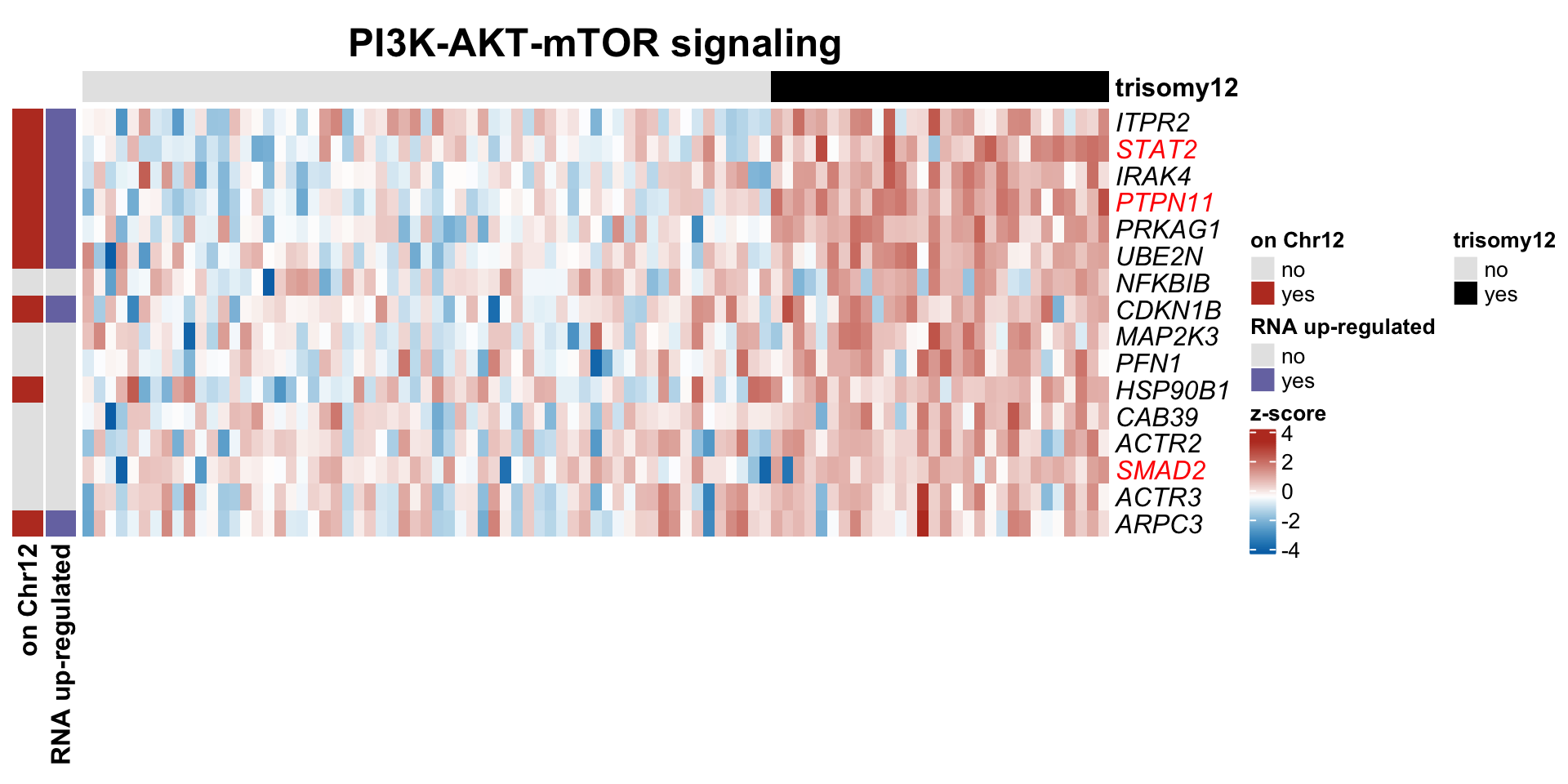
#dev.off()plotSetHeatmap(resList.sig, gmts$H, "HALLMARK_MTORC1_SIGNALING", plotMat, colAnno, rowAnno = rowAnno, annoCol = annoCol, plotName = "MTORC1 signaling",
highLight = nameList)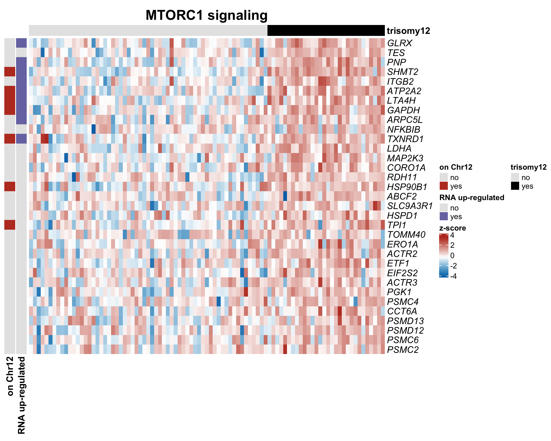
plotSetHeatmap(resList.sig, gmts$H, "HALLMARK_INTERFERON_ALPHA_RESPONSE", plotMat, colAnno, rowAnno = rowAnno, annoCol = annoCol, plotName = "Interferon alpha response",
                highLight = nameList)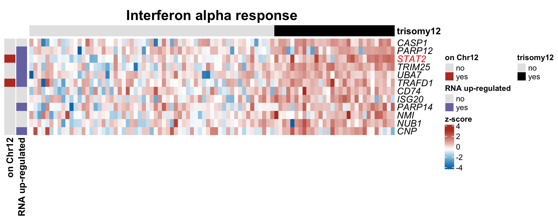
#pdf("trisomy12_BCR_heatmap.pdf", height=6, width=10)
plotSetHeatmap(resList.sig, gmts$KEGG, "KEGG_B_CELL_RECEPTOR_SIGNALING_PATHWAY", plotMat, highLight = nameList,
colAnno, rowAnno = rowAnno, annoCol = annoCol, plotName = "B-cell receptor signaling") 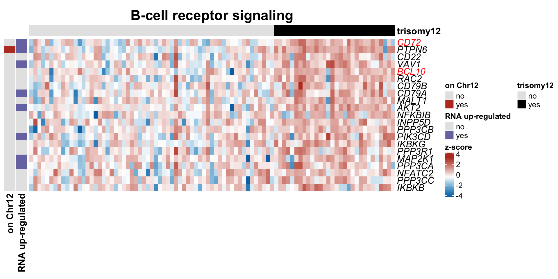
#dev.off()Compare protein expression with RNA expression related to trisomy12
Differentially expressed RNA related to trisomy12
Prepare RNA sequencing data
dds$trisomy12 <- factor(patMeta[match(dds$PatID, patMeta$Patient.ID),]$trisomy12)
dds$IGHV <- factor(patMeta[match(dds$PatID, patMeta$Patient.ID),]$IGHV.status)

ddsCLL <- dds[rownames(dds) %in% rowData(protCLL)$ensembl_gene_id, !is.na(dds$IGHV) & !is.na(dds$trisomy12)]
ddsCLL.vst <- ddsCLL
assay(ddsCLL.vst) <- log2(counts(ddsCLL, normalized = TRUE) + 1)
#ddsCLL.vst <- varianceStabilizingTransformation(ddsCLL)
Differential expression
resTab <- filter(resListRNA, Gene == "trisomy12")Boxplot of selected genes
plotTab <- assay(ddsCLL.vst[match(nameList, rowData(ddsCLL.vst)$symbol),]) %>%
  data.frame() %>% rownames_to_column("id") %>%
  mutate(name = rowData(ddsCLL.vst[id,])$symbol) %>%
  gather(key = "patID", value = "count", -id, -name) %>%
  mutate(trisomy12 = patMeta[match(patID, patMeta$Patient.ID),]$trisomy12) %>%
  mutate(status = ifelse(trisomy12 %in% 1,"trisomy12","other"))  %>%
  mutate(status = factor(status, levels = c("other","trisomy12")))


pList <- plotBox(plotTab, pValTabel = resTab, y_lab = "RNA expression")
cowplot::plot_grid(plotlist= pList, ncol=2)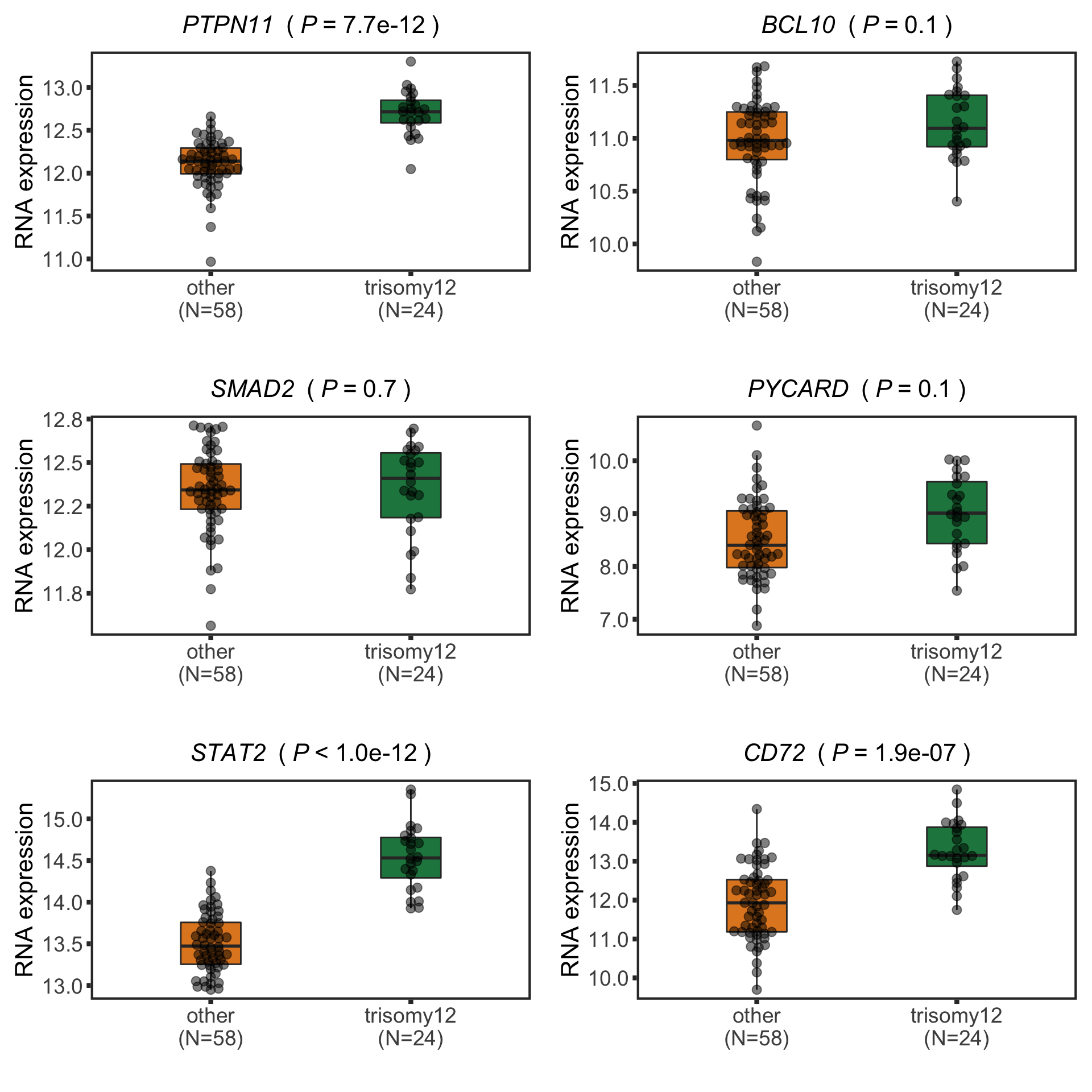
Correlations between RNA and protein expression
rnaMat <- assay(ddsCLL.vst)
protMat <- assays(protCLL)[["log2Norm_combat"]]
rownames(protMat) <- rowData(protCLL)$ensembl_gene_id
overSample <- intersect(colnames(rnaMat), colnames(protMat))
rnaMat <- rnaMat[,overSample]
protMat <- protMat[,overSample]

plotList <- lapply(nameList, function(n) {
  geneId <- rownames(ddsCLL.vst)[match(n, rowData(ddsCLL.vst)$symbol)]
  stopifnot(length(geneId) ==1)
  plotTab <- tibble(x=rnaMat[geneId,],y=protMat[geneId,])
  coef <- cor(plotTab$x, plotTab$y, use="pairwise.complete")
  annoPos <- ifelse (coef > 0, "left","right")
  plotCorScatter(plotTab, "x","y", showR2 = FALSE, annoPos = annoPos, x_lab = "RNA expression",
                 y_lab ="Protein expression", title = n,dotCol = colList[4], textCol = colList[1])
})
cowplot::plot_grid(plotlist = plotList, ncol =2)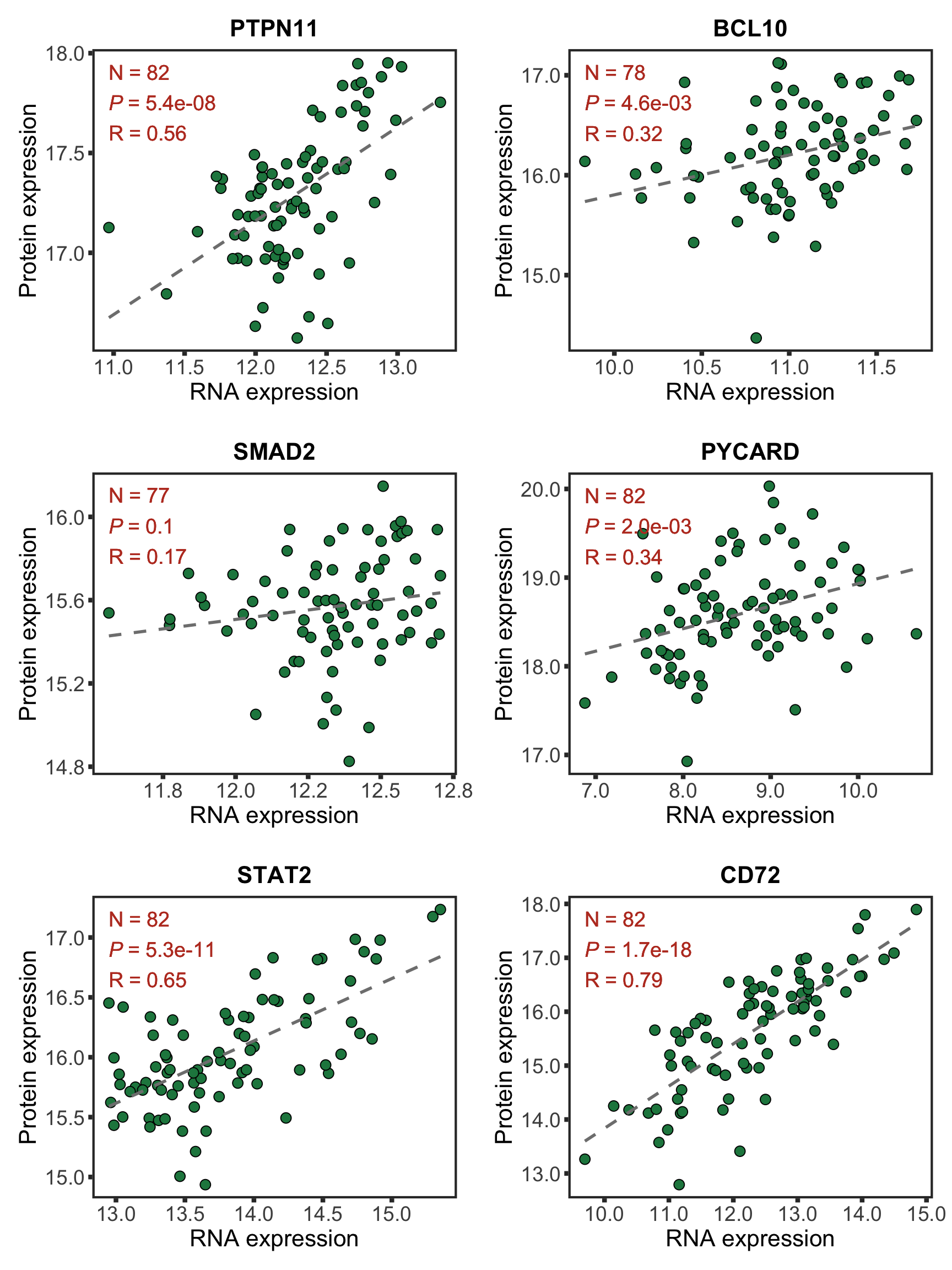
Gene dosage effect and protein buffering related to trisomy12
Visualizing gene dosage effect on protein and RNA level
Processing protein and RNA count data
protExprTab <- sumToTidy(protCLL) %>%
  filter(chromosome_name == "12") %>%
  mutate(id = ensembl_gene_id, patID = colID, expr = log2Norm_combat, type = "Protein") %>%
  select(id, patID, expr, type)

rnaExprTab <- counts(dds[rownames(dds) %in% protExprTab$id,
                            colnames(dds) %in% protExprTab$patID], normalized= TRUE) %>%
  as_tibble(rownames = "id") %>%
  pivot_longer(-id, names_to = "patID", values_to = "count") %>%
  mutate(expr = log2(count)) %>%
  select(id, patID, expr) %>% mutate(type = "RNA")

comExprTab <- bind_rows(rnaExprTab, protExprTab) %>%
  mutate(trisomy12 = patMeta[match(patID, patMeta$Patient.ID),]$trisomy12) %>%
  filter(!is.na(trisomy12)) %>% mutate(cnv = ifelse(trisomy12 %in% 1, "trisomy12","other"))
Proteins/RNAs on Chr12 have higher expressions in trisomy12 samples compared to other samples
plotTab <- comExprTab %>%
  group_by(id,type) %>% mutate(zscore = (expr-mean(expr))/sd(expr)) %>%
  group_by(id, cnv, type) %>% summarise(meanExpr = mean(zscore, na.rm=TRUE)) %>%
  ungroup()

dosagePlot <- ggplot(plotTab, aes(x=meanExpr, fill = cnv, col=cnv)) +
  geom_histogram(position = "identity", alpha=0.5, bins=30) + facet_wrap(~type, scale = "fixed") +
  scale_fill_manual(values = c(other = "grey80", trisomy12 = colList[1]), name = "") +
  scale_color_manual(values = c(other = "grey80", trisomy12 = colList[1]), name = "") +
  xlim(-1,1.5) +
  theme_full + xlab("Mean Z-score") +
  theme(strip.text = element_text(size =20),
        legend.position = c(0.1,0.9), legend.background = element_rect(fill = NA),
        legend.text = element_text(size=15))

dosagePlot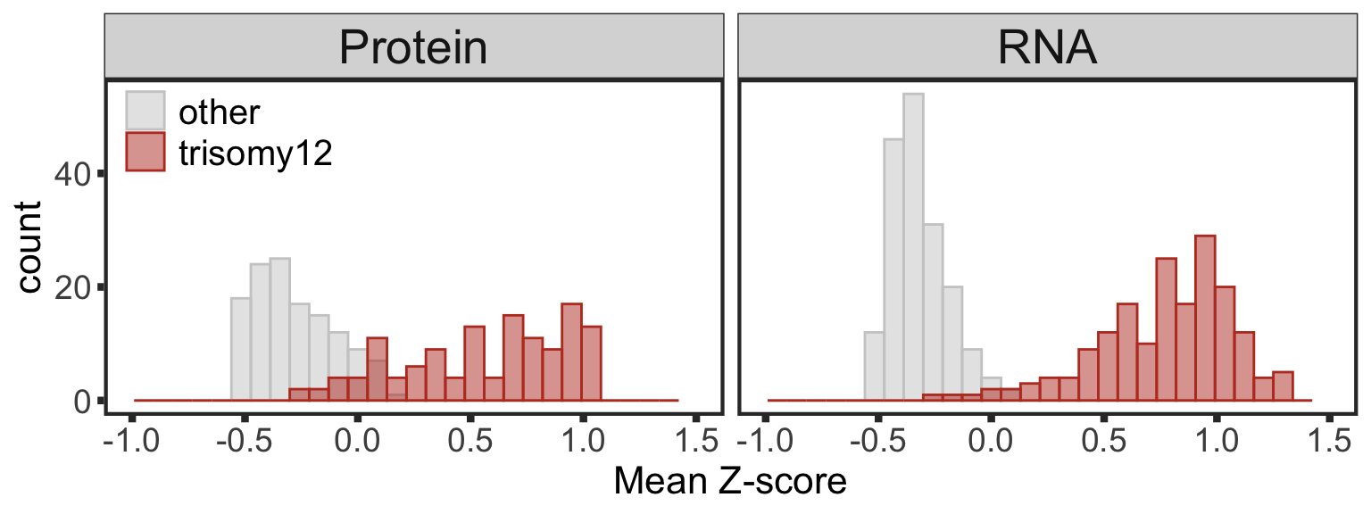
Analyzing protein buffering effect
Detect buffered and non-buffered proteins
Preprocessing protein and RNA data
#subset samples and genes
overSampe <- intersect(colnames(ddsCLL), colnames(protCLL))
overGene <- intersect(rownames(ddsCLL), rowData(protCLL)$ensembl_gene_id)
ddsSub <- ddsCLL[overGene, overSampe]
protSub <- protCLL[match(overGene, rowData(protCLL)$ensembl_gene_id),overSampe]
rowData(ddsSub)$uniprotID <- rownames(protSub)[match(rownames(ddsSub),rowData(protSub)$ensembl_gene_id)]

#vst
ddsSub.vst <- ddsSub
assay(ddsSub.vst) <- log2(counts(ddsSub, normalized=TRUE) +1)

rnaRes <- resListRNA %>% filter(Gene == "trisomy12") %>%
  mutate(chrom = rowData(dds[id,])$chromosome) %>%
  dplyr::rename(geneID = id, log2FC.rna = log2FC,
                pvalue.rna = P.Value, padj.rna = adj.P.Val, stat.rna= t) %>%
  arrange(pvalue.rna) %>% distinct(name, .keep_all = TRUE) %>%
  select(geneID, name, log2FC.rna, pvalue.rna, padj.rna, stat.rna, chrom)

protRes <- resList %>% filter(Gene == "trisomy12") %>%
    mutate(Chr = rowData(protCLL[id,])$chromosome_name) %>%
    #filter(Chr == "12") %>%
    #mutate(adj.P.Val = p.adjust(P.Value, method= "BH")) %>%
    dplyr::rename(uniprotID = id,
                  pvalue = P.Value, padj = adj.P.Val) %>%
    #mutate(geneID = rowData(protCLL[uniprotID,])$ensembl_gene_id) %>%
    select(name, uniprotID, log2FC, pvalue, padj, t) %>%
    dplyr::rename(stat =t) %>%
    arrange(pvalue) %>% distinct(name,.keep_all = TRUE) %>%
  as_tibble()

allRes <- left_join(protRes, rnaRes, by = "name") %>%
  filter(!is.na(stat), !is.na(stat.rna))
Identify buffered and non-buffered proteins by comparing protein expression changes and RNA expression changes
fdrCut <- 0.05

bufferTab <- allRes %>% filter(chrom == "12", stat.rna > 0) %>%
  ungroup() %>%
  mutate(stat.prot.sqrt = sqrt(stat),
         stat.prot.center = stat.prot.sqrt - mean(stat.prot.sqrt,na.rm= TRUE)) %>%
  mutate(score = -stat.prot.center*stat.rna,
         diffFC = log2FC.rna-log2FC) %>%
  mutate(ifBuffer = case_when(
    padj <= fdrCut & padj.rna <= fdrCut & stat > 0 ~ "non-Buffered",
    padj > fdrCut & padj.rna <= fdrCut ~ "Buffered",
    padj < fdrCut & padj.rna > fdrCut & stat > 0 ~ "Enhanced",
    TRUE ~ "Undetermined"
  )) %>%
  arrange(desc(score))
Table of comparison
bufferTab %>% select(name, geneID, ifBuffer, score, log2FC, padj, log2FC.rna, padj.rna) %>%
  mutate_if(is.numeric, formatC, digits=2) %>%
  DT::datatable()
Summary plot
sumTab <- bufferTab %>% group_by(ifBuffer) %>%
  summarise(n = length(name))

bufferPlot <- ggplot(sumTab, aes(x=ifBuffer, y = n)) +
  geom_bar(aes(fill = ifBuffer), stat="identity", width = 0.7) +
  geom_text(aes(label = paste0(n)),vjust=-0.5,col="black",size=5) +
  scale_fill_manual(values =c(Buffered = colList[1],
                              Enhanced = colList[4],
                              `non-Buffered` = colList[2],
                              Undetermined = "grey50")) +
  theme_half + theme(axis.text.x = element_text(angle = 90, hjust=1, vjust=0.5),
                     legend.position = "none") +
  ylab("Number of proteins") + ylim(0,120) +xlab("")
bufferPlot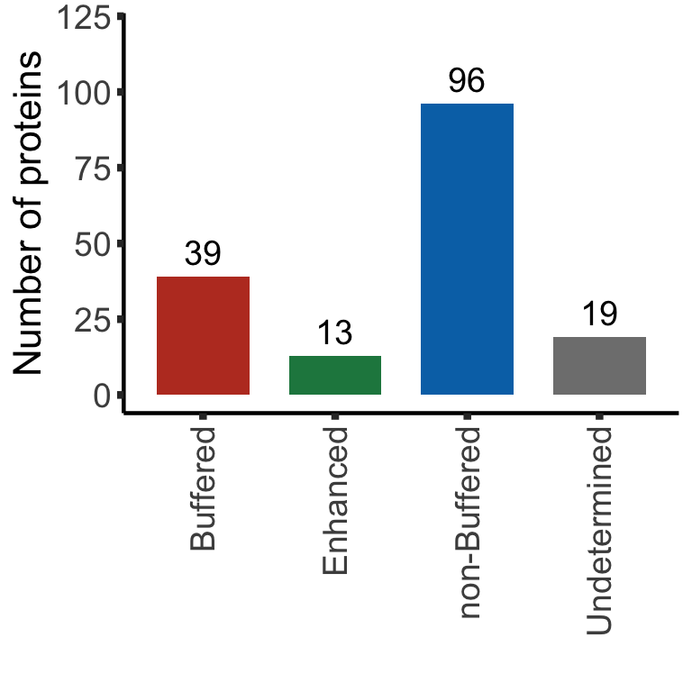
#ggsave("tri12_sum_buffer_number.pdf", width =4, height = 4)Enrichment of buffer and non-buffered proteins
Non-buffered prpteins
Using cancer hallmark genesets
rnaAll <- dds[rowData(dds)$biotype %in% "protein_coding" & !rowData(dds)$symbol %in% c("",NA),] #all protein coding gene as background

protList <- filter(bufferTab, ifBuffer == "non-Buffered")$name
refList <- rowData(rnaAll)$symbol
enRes <- runFisher(protList, refList, gmts$H, pCut =0.01, ifFDR = TRUE,removePrefix = "HALLMARK_",
                   plotTitle = "Non-buffered proteins", insideLegend = TRUE,
                   setName = "HALLMARK gene set", setMap = setMap)
bufferEnrich <- enRes$enrichPlot + theme(plot.margin = margin(1,3,1,1, unit = "cm"))
bufferEnrich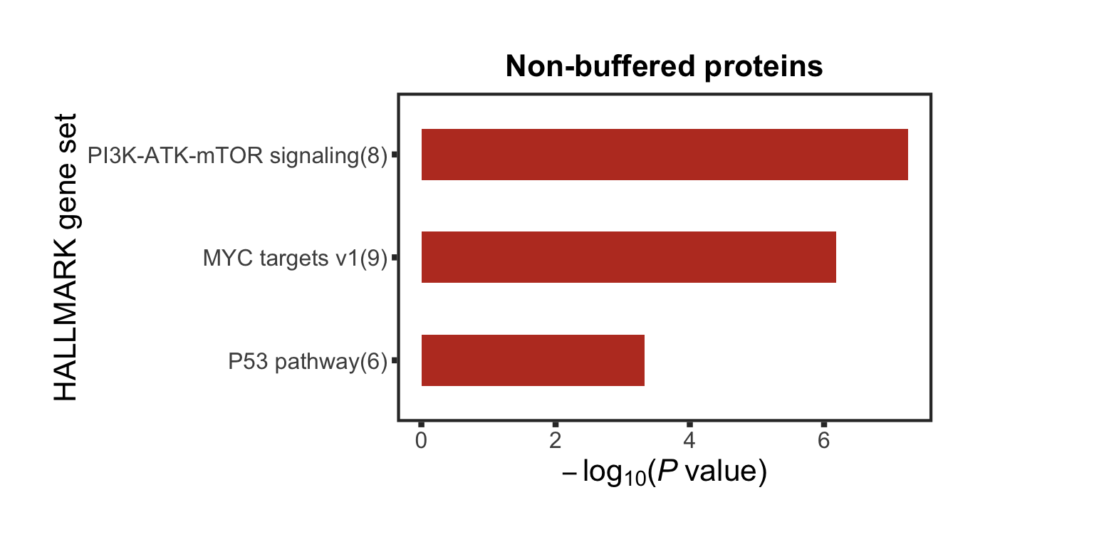
#ggsave("tri12_nonBuffer_enrich.pdf", height = 3.5, width = 7)Buffered proteins
protList <- filter(bufferTab, ifBuffer == "Buffered")$name
enRes <- runFisher(protList, refList, gmts$H, pCut =0.1, ifFDR = TRUE)
[1] "No sets passed the criteria"No enrichment
Compare the protein buffering effect between trisomy19 and trisomy12
load("../output/deResList.RData")
load("../output/deResListRNA.RData")
testTabProt <- resList %>% mutate(chr = rowData(protCLL[id,])$chromosome_name) %>%
  filter(Gene == paste0("trisomy",chr)) %>%
  select(name, log2FC, Gene) %>% mutate(type = "Protein")
testTabRNA <- resListRNA %>% mutate(chr = rowData(dds[id,])$chromosome) %>%
  filter(Gene == paste0("trisomy",chr)) %>%
  select(name, log2FC, Gene) %>% mutate(type = "RNA")
overGene <- intersect(testTabProt$name, testTabRNA$name)
testTab <- bind_rows(testTabProt, testTabRNA) %>%
  filter(name %in% overGene)
plotTab <- lapply(seq(-2,2, length.out = 50), function(foldCut) {
filTab <- mutate(testTab, pass = log2FC > foldCut) %>%
group_by(Gene, type) %>% summarise(n = sum(pass),per = sum(pass)/length(pass)) %>%
mutate(cut = foldCut)
}) %>% bind_rows() %>%
mutate(group =paste0(Gene,"_",type))Cummulative curve plot
ggplot(plotTab, aes(x=cut, y = per))+
  geom_line(aes(col = Gene, linetype = type),size=1) +
  scale_color_manual(values = c(trisomy12 = colList[1],trisomy19=colList[2]), name = "") +
  scale_linetype_discrete(name = "") +
  coord_cartesian(xlim=c(-0.5,1)) +
  ylab("Cumulative fraction") +
  xlab(bquote("log"[2]*"(fold change)")) +
  theme_full +
  theme(legend.position = c(0.80,0.80),
        axis.text = element_text(size=15),
        axis.title = element_text(size=15),
        legend.text = element_text(size=15),
        legend.background = element_rect(fill = NA))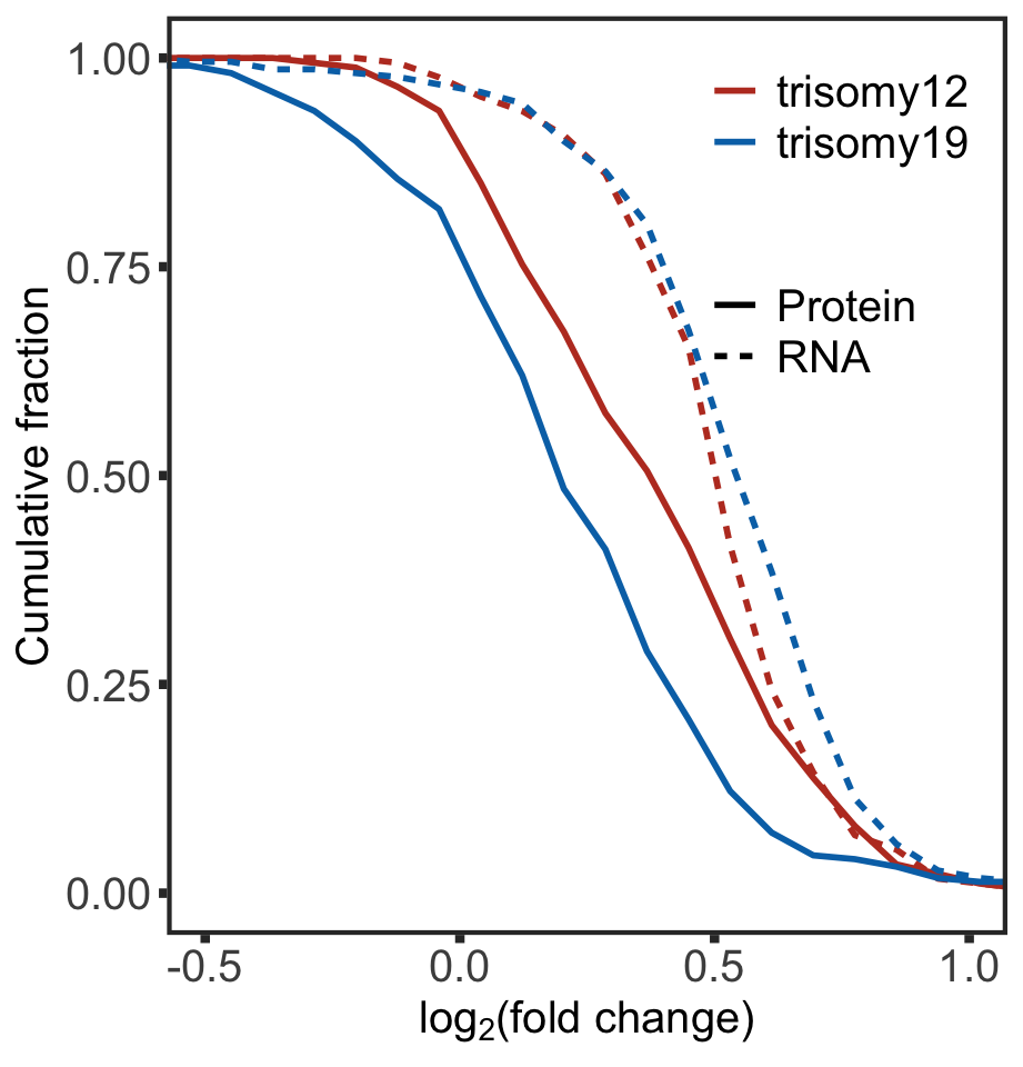
#ggsave("buffer_Tri12vsTri19.pdf", height = 5, width = 4.8)KS test to compare the RNA expression changes and protein expression changes between trisomy12 cases and trisomy19 cases
RNA level
testTab <- plotTab %>% filter(type == "RNA") %>%
  select(Gene, per,cut) %>% pivot_wider(names_from = Gene, values_from = per)
ks.test(testTab$trisomy12, testTab$trisomy19)
    Two-sample Kolmogorov-Smirnov test

data:  testTab$trisomy12 and testTab$trisomy19
D = 0.22, p-value = 0.1777
alternative hypothesis: two-sided
Protein level
testTab <- plotTab %>% filter(type == "Protein") %>%
  select(Gene, per,cut) %>% pivot_wider(names_from = Gene, values_from = per)
ks.test(testTab$trisomy12, testTab$trisomy19)
    Two-sample Kolmogorov-Smirnov test

data:  testTab$trisomy12 and testTab$trisomy19
D = 0.42, p-value = 0.0002955
alternative hypothesis: two-sided
Plot protein and RNA expression of genes togehter with their genomic coordinate information
patBack <- dplyr::filter(patMeta, Patient.ID %in% unique(allProtTab$patID)) %>%
  dplyr::select(Patient.ID, trisomy12) %>%
  dplyr::rename(patID = Patient.ID) %>%
  mutate_all(as.character) %>%
  mutate_at(vars(-patID),str_replace, "1","yes") %>%
  mutate_at(vars(-patID),str_replace, "0","no")
plotExprVar <- function(gene, chr, patBack, allBand, allLine, allProtTab, allRnaTab, protLine = NULL,
region = c(-Inf,Inf),ifTrend = FALSE, normalize = TRUE, maxVal =2, minVal=-2) {
#table for cyto band
bandTab <- filter(allBand, ChromID == chr, chromStart >= region[1], chromEnd <= region[2]) %>%
mutate(chromMid = chromMid)
#table for expression
plotProtTab <- filter(allProtTab, ChromID == chr, start_position >= region[1], end_position <= region[2]) %>%
mutate_if(is.factor,as.character)
plotRnaTab <- filter(allRnaTab, ChromID == chr, start_position >= region[1], end_position <= region[2]) %>%
mutate_if(is.factor,as.character)
#summarise group mean
plotProtTab <- plotProtTab %>%
mutate(group = patBack[match(patID, patBack$patID),][[gene]]) %>%
filter(!is.na(group)) %>%
group_by(id, group) %>% mutate(meanExpr = mean(expr, na.rm=TRUE)) %>%
distinct(group, id,.keep_all = TRUE) %>% ungroup()
plotRnaTab <- plotRnaTab %>%
mutate(group = patBack[match(patID, patBack$patID),][[gene]]) %>%
filter(!is.na(group)) %>%
group_by(id, group) %>% mutate(meanExpr = mean(expr, na.rm=TRUE)) %>%
distinct(group, id,.keep_all = TRUE) %>% ungroup()
if (!is.null(protLine)) {
bufferLineTab <- plotProtTab %>%
select(symbol, mid_position, meanExpr, group) %>%
filter(symbol %in% protLine) %>%
pivot_wider(names_from = group, values_from = meanExpr) %>%
mutate(lowVal = map2_dbl(yes, no, min),
highVal = map2_dbl(yes, no, max))
} else bufferLineTab <- NULL
xMax <- max(bandTab$chromEnd, na.rm = T)
#main plot for Protein
gPro <- ggplot() +
geom_rect(data=bandTab, mapping=aes(xmin=chromStart, xmax=chromEnd, ymin=minVal+0.5, ymax=maxVal-0.5,
fill=Colour, label = band), alpha=0.1) +
geom_text(data=bandTab, mapping=aes(label=band, x=chromMid), y=maxVal-0.5, hjust =1, angle = 90, size=2.5)
if (!is.null(protLine)) {
gPro <- gPro + geom_segment(data = bufferLineTab, aes(x=mid_position, xend = mid_position,
y=lowVal, yend = highVal), linetype = "dashed")
}
gPro <- gPro + geom_rect(data = plotProtTab,
mapping=aes(xmin=start_position,
xmax=end_position, ymin=meanExpr, ymax=meanExpr+0.1,
fill = group, label = symbol)) +
scale_x_continuous(expand=c(0,0),limits = c(0,xMax)) +
xlab("Genomic position [Mb]") +
ylab("Expression Z-score") +
scale_fill_manual(values = c(even = "white",odd = "grey50",
yes = colList[1], no = colList[4])) +
scale_color_manual(values = c(yes = colList[1],no = colList[4])) +
ggtitle(paste0("Protein expression","(",chr,")")) +
theme(plot.title = element_text(face = "bold", size = 10),
legend.position = "none",
panel.background = element_blank(),
panel.grid.major = element_line(colour="grey90", size=0.1))
if (ifTrend) {
gPro <- gPro + stat_smooth(data =filter(plotProtTab, expr >0),
mapping = aes(y=meanExpr, x= mid_position,
color = group),
geom="line",
formula = y ~ x, method = "loess", se=FALSE, span=0.5,
size =1, alpha=0.5)
}
#main plot for RNA
gRna <- ggplot() +
geom_rect(data=bandTab, mapping=aes(xmin=chromStart, xmax=chromEnd, ymin=minVal, ymax=maxVal,
fill=Colour, label = band), alpha=0.1) +
geom_text(data=bandTab, mapping=aes(label=band, x=chromMid), y=maxVal, hjust =1, angle = 90, size=2.5) +
geom_rect(data = plotRnaTab,
mapping=aes(xmin=start_position,
xmax=end_position, ymin=meanExpr, ymax=meanExpr+0.1,
fill = group, label = symbol)) +
scale_x_continuous(expand=c(0,0),limits = c(0,xMax)) +
xlab("Genomic position [Mb]") +
ylab("Expression Z-score") +
scale_fill_manual(values = c(even = "white",odd = "grey50",
yes = colList[1], no = colList[4])) +
scale_color_manual(values = c(yes = colList[1], no = colList[4])) +
ggtitle(paste0("RNA expression","(",chr,")")) +
theme(plot.title = element_text(face = "bold", size = 10),
legend.position = "none",
panel.background = element_blank(),
panel.grid.major = element_line(colour="grey90", size=0.1))
if (ifTrend) {
gRna <- gRna + stat_smooth(data =filter(plotRnaTab),
mapping = aes(y=meanExpr, x= mid_position,
color = group),
geom="line",
formula = y ~ x, method = "loess", se=FALSE, span=0.2,
size =1, alpha=0.5)
}
#for legend
## if the patient has CNV data
lgTab <- tibble(x= seq(6),y=seq(6),
Expression = c(rep("yes",3), rep("no",3)))
lg <- ggplot(lgTab, aes(x=x,y=y)) +
geom_point(aes(fill = Expression), shape =22,size=3) +
scale_fill_manual(values = c(yes = "darkred", no = "darkgreen"), name = gene) +
theme(legend.position = "bottom")
lg <- get_legend(lg)
return(list(plotPro = gPro, plotRNA = gRna, legend = lg))
}Normalize protein and RNA expression
normalized <- TRUE
#if perform normalization
if (normalized) {
  #for protein
  exprMat <- select(allProtTab,patID, id,expr) %>%
    distinct(patID, id, .keep_all = TRUE) %>%
    spread(key = patID, value =expr) %>% data.frame() %>%
    column_to_rownames("id") %>% as.matrix()
  qm <- jyluMisc::mscale(exprMat, useMad = F)
  normTab <- data.frame(qm) %>% rownames_to_column("id") %>%
    gather(key = "patID", value = "expr", -id)
  allProtTab <- select(allProtTab, -expr) %>% left_join(normTab, by = c("patID","id"))


  #for RNA
  exprMat <- select(allRnaTab,patID, id,expr) %>%
    distinct(patID, id, .keep_all = TRUE) %>%
    spread(key = patID, value =expr) %>% data.frame() %>%
    column_to_rownames("id") %>% as.matrix()
  qm <- jyluMisc::mscale(exprMat, useMad = F)
  normTab <- data.frame(qm) %>% rownames_to_column("id") %>%
    gather(key = "patID", value = "expr", -id)
  allRnaTab <- select(allRnaTab, -expr) %>% left_join(normTab, by = c("patID","id"))
}
g <- plotExprVar("trisomy12","chr12",patBack,allBand, allLine,
allProtTab, allRnaTab, ifTrend = TRUE)
plot_grid(g$plotRNA, g$plotPro, g$legend, ncol = 1, rel_heights = c(1,1,0.2))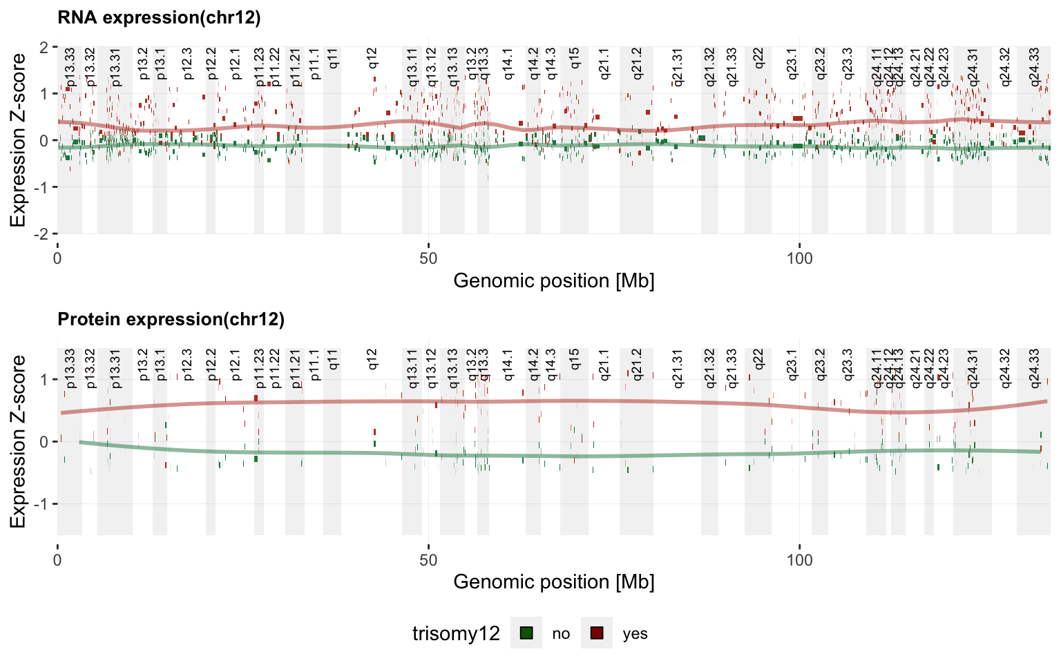
#ggsave("chr12Plot.pdf", height = 5, width = 8)Using circular heatmap to visuailize RNA and protein expressions of chr12 genes
Prepare data for plotting
Protein expression data
protChr12 <- protCLL[rowData(protCLL)$chromosome_name %in% "12",]

#subset for fast testing
#protChr12 <- protChr12[sample(rownames(protChr12), size = as.integer(nrow(protChr12)/5))]

protMat <- assays(protChr12)[["QRILC_combat"]]
rownames(protMat) <- rowData(protChr12)$hgnc_symbol
#column annotation
colAnno <- tibble(patID = colnames(protChr12),
                  trisomy12 = patMeta[match(patID, patMeta$Patient.ID),]$trisomy12) %>%
  mutate(trisomy12 = ifelse(trisomy12 %in% "1","Tri12","other")) %>%
  arrange(trisomy12) %>%
  data.frame() %>% column_to_rownames("patID")

protMat <- protMat[!duplicated(rownames(protMat)),rownames(colAnno)]
RNA expression data
rnaChr12 <- ddsCLL.vst[rowData(ddsCLL.vst)$symbol %in% rownames(protMat),]
rnaMat <- assay(rnaChr12)
rownames(rnaMat) <- rowData(rnaChr12)$symbol

colAnnoRNA <- tibble(patID = colnames(rnaChr12),
                  trisomy12 = patMeta[match(patID, patMeta$Patient.ID),]$trisomy12) %>%
  mutate(trisomy12 = ifelse(trisomy12 %in% "1","Tri12","other")) %>%
  arrange(trisomy12) %>%
  data.frame() %>% column_to_rownames("patID")


rnaMat <- rnaMat[!duplicated(rownames(rnaMat)) ,rownames(colAnnoRNA)]

#subset for commonly detected genes
overGene <- intersect(rownames(rnaMat), rownames(protMat))
protMat <- protMat[overGene,]
rnaMat <- rnaMat[overGene,]
Get chromosome band membership for each protein
library(biomaRt)
allID <- rowData(protChr12)$ensembl_gene_id
idToSymbol <- rowData(protChr12)[,c("ensembl_gene_id","hgnc_symbol")] %>% as_tibble()
mart<-useMart(biomart="ENSEMBL_MART_ENSEMBL",
              dataset="hsapiens_gene_ensembl",
              host="grch37.ensembl.org")

locAnno <- getBM(values = allID ,mart = mart,
      attributes = c("ensembl_gene_id","start_position","end_position"),
      filters = "ensembl_gene_id") %>%
  distinct(ensembl_gene_id, .keep_all = TRUE)

geneAnno <- tibble(id = allID) %>%
  left_join(locAnno, by = c(id= "ensembl_gene_id")) %>%
  left_join(idToSymbol, by = c(id = "ensembl_gene_id"))

stopifnot(all(!is.na(geneAnno$hgnc_symbol)))

chr12Band <- filter(allBand, ChromID == "chr12")
bandTab <- lapply(seq(nrow(geneAnno)), function(i) {
  rec <- geneAnno[i,]
  bandName <- mutate(chr12Band, within = chromStart < rec$start_position/10^6 & chromEnd > rec$start_position/10^6) %>%
    filter(within) %>% pull(band)
  tibble(id = rec$id, band = as.character(bandName))
}) %>% bind_rows()

geneAnno <- left_join(geneAnno, bandTab, by = "id") %>%
  arrange(start_position) %>%
  distinct(hgnc_symbol, .keep_all = TRUE) %>%
  mutate(band = factor(band, levels = unique(band)))


detach("package:biomaRt", unload=TRUE)
Prepare row annotation
#for annotate protein regulation
upProtList <- filter(resList, Gene == "trisomy12", t >0, adj.P.Val <= 0.05)$name
upRNAList <- filter(resListRNA, Gene == "trisomy12", t >0, adj.P.Val <= 0.05)$name

rowAnno <- tibble(symbol = rownames(protMat)) %>%
  left_join(dplyr::select(geneAnno, hgnc_symbol, band, start_position), by = c(symbol = "hgnc_symbol")) %>%
  mutate(direction = case_when(
    symbol %in% intersect(upProtList, upRNAList) ~ "both up",
    symbol %in% upProtList & !symbol %in% upRNAList ~ "protein up",
    symbol %in% upRNAList & !symbol %in% upProtList ~ "RNA up",
    TRUE ~ "none"
  )) %>%
  mutate(`protUp` = ifelse(direction %in% c("both up","protein up"),"yes","no"),
         `rnaUp` = ifelse(direction %in% c("both up","RNA up"), "yes","no")) %>%
  arrange(start_position) %>% data.frame() %>% column_to_rownames("symbol")
protMat <- protMat[rownames(rowAnno),]
rnaMat <- rnaMat[rownames(rowAnno),]
Plot heatmap using circos package (with gene names)
library(circlize)
library(ComplexHeatmap)

protMat <- mscale(protMat, censor = 5)
rnaMat <- mscale(rnaMat, censor =5)
pdf("heatmap_tri12_circle.pdf", height=10, width=10)

#global gap size
circos.par(gap.after = c(rep(2, length(unique(rowAnno$band))-1),6))


#protein heatmap
col_funProt = colorRamp2(c(-5, 0, 5), c(colList[2], "white", colList[1]))
circos.heatmap(protMat, split = rowAnno$band, cluster = FALSE, col = col_funProt, show.sector.labels = FALSE, rownames.side = "outside")

#column annotation of sample type for protein
nTri12 <- table(colAnno$trisomy12)["Tri12"]
nWT <- table(colAnno$trisomy12)[["other"]]
circos.track(track.index = get.current.track.index(), panel.fun = function(x, y) {
    if(CELL_META$sector.numeric.index == length(unique(rowAnno$band))) { # the last sector
        circos.rect(CELL_META$cell.xlim[2] + convert_x(1, "mm"), 0,
                    CELL_META$cell.xlim[2] + convert_x(7, "mm"), nWT,
                    col = NA, border = "grey60")
        circos.text(CELL_META$cell.xlim[2] + convert_x(4, "mm"), nWT/2,
                    "other", cex = 0.5, facing = "clockwise", font=2)

        circos.rect(CELL_META$cell.xlim[2] + convert_x(1, "mm"), nWT,
                    CELL_META$cell.xlim[2] + convert_x(7, "mm"), nWT+nTri12,
                    col = NA, border = "grey60")
        circos.text(CELL_META$cell.xlim[2] + convert_x(4, "mm"), nWT + nTri12/2,
                    "tri12", cex = 0.5, facing = "clockwise", font=2)
    }
}, bg.border = NA)

#annotation of prtein regulation
col_ProtDir = c(yes = colList[3], no = "grey90")
circos.heatmap(rowAnno$protUp, col = col_ProtDir, track.height = 0.02, bg.border = "grey50")

#annotation of rna regulation
col_RnaDir = c(yes = colList[5], no = "grey90")
circos.heatmap(rowAnno$rnaUp, col = col_RnaDir, track.height = 0.02, bg.border = "grey50")

#rna heatmap
col_funRna = colorRamp2(c(-5, 0, 5), c(colList[4], "white", colList[1]))
circos.heatmap(rnaMat, split = rowAnno$band, cluster = FALSE, col = col_funRna)

#column annotation of sample type for rna
nTri12 <- table(colAnnoRNA$trisomy12)["Tri12"]
nWT <- table(colAnnoRNA$trisomy12)[["other"]]
circos.track(track.index = get.current.track.index(), panel.fun = function(x, y) {
    if(CELL_META$sector.numeric.index == length(unique(rowAnno$band))) { # the last sector
        circos.rect(CELL_META$cell.xlim[2] + convert_x(1, "mm"), 0,
                    CELL_META$cell.xlim[2] + convert_x(5, "mm"), nWT,
                    col = NA, border = "grey60")
        circos.text(CELL_META$cell.xlim[2] + convert_x(3, "mm"), nWT/2,
                    "other", cex = 0.5, facing = "clockwise", font=2)

        circos.rect(CELL_META$cell.xlim[2] + convert_x(1, "mm"), nWT,
                    CELL_META$cell.xlim[2] + convert_x(5, "mm"), nWT+nTri12,
                    col = NA, border = "grey60")
        circos.text(CELL_META$cell.xlim[2] + convert_x(3, "mm"), nWT + nTri12/2,
                    "tri12", cex = 0.5, facing = "clockwise", font=2)
    }
}, bg.border = NA)

circos.track(ylim = c(0, 1), panel.fun = function(x, y) {
    circos.text(CELL_META$xcenter, CELL_META$ycenter,
        unique(rowAnno$band)[CELL_META$sector.numeric.index],
        facing = "clockwise", niceFacing = TRUE,  cex = 0.7, col = "grey50")
}, bg.border = NA, track.height = 0.06)


circos.clear()


dev.off()
pdf
2 Plot legend separately
#draw legend
#pdf("heatmap_tri12_circle_legend.pdf", height=5, width=5)

#draw legend

lgd_Prot = Legend(title = "Protein expression", col_fun = col_funProt, title_position = "lefttop-rot")
lgd_Rna = Legend(title = "RNA expression", col_fun = col_funRna, title_position = "lefttop-rot")
lgd_ProtDir = Legend(title = "Protein up-regulated ", at = names(col_ProtDir), legend_gp = gpar(fill = col_ProtDir))
lgd_RnaDir = Legend(title = "RNA up-regulated", at = names(col_RnaDir), legend_gp = gpar(fill = col_RnaDir))

lgd_list = packLegend(lgd_Prot, lgd_Rna, lgd_ProtDir, lgd_RnaDir, direction = "vertical")
grid.draw(lgd_list) 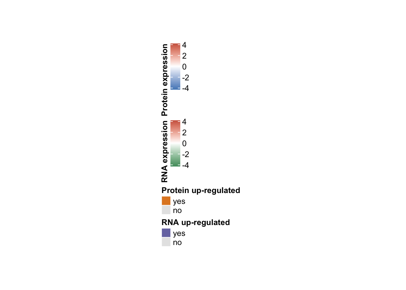
Protein complex analysis
Data preprocessing
Read stable protein complex pairs
int_pairs <- read_csv2("../output/int_pairs.csv")Whether complex formation affects protein buffering?
Compare log2 fold changes difference
testTab <- bufferTab %>% mutate(inComplex = ifelse(uniprotID %in% c(int_pairs$ProtA,int_pairs$ProtB),
                                                   "complex in","complex out")) %>%
  group_by(inComplex) %>% mutate(n = length(name)) %>%
  mutate(xLabel = sprintf("%s\n(N=%s)",inComplex,n))

tRes <- t.test(diffFC~inComplex, testTab)

pVal <- formatC(tRes$p.value, digits = 1, format="e")
pLab <- bquote(italic("P")~"="~.(pVal))

ggplot(testTab, aes(x=xLabel, y=diffFC)) +
  geom_violin(aes(fill = xLabel), trim=FALSE) +
  stat_summary(fun.data="mean_sdl", mult=1,
                 geom="errorbar", width=0.05) +
  stat_summary(fun.y=mean, geom="point") +
  scale_fill_manual(values = colList[4:5]) +
  theme_full +
  xlab("") + ylab("log2(RNA fold change) - log2(protein fold change)") +
  annotate("text", label = pLab , x=Inf, y=Inf, hjust=1.2, vjust=2,size=6) +
  theme(legend.position = "none",
        axis.text.y = element_text(size=15),
        axis.text.x = element_text(size=18),
axis.title = element_text(size=15)) 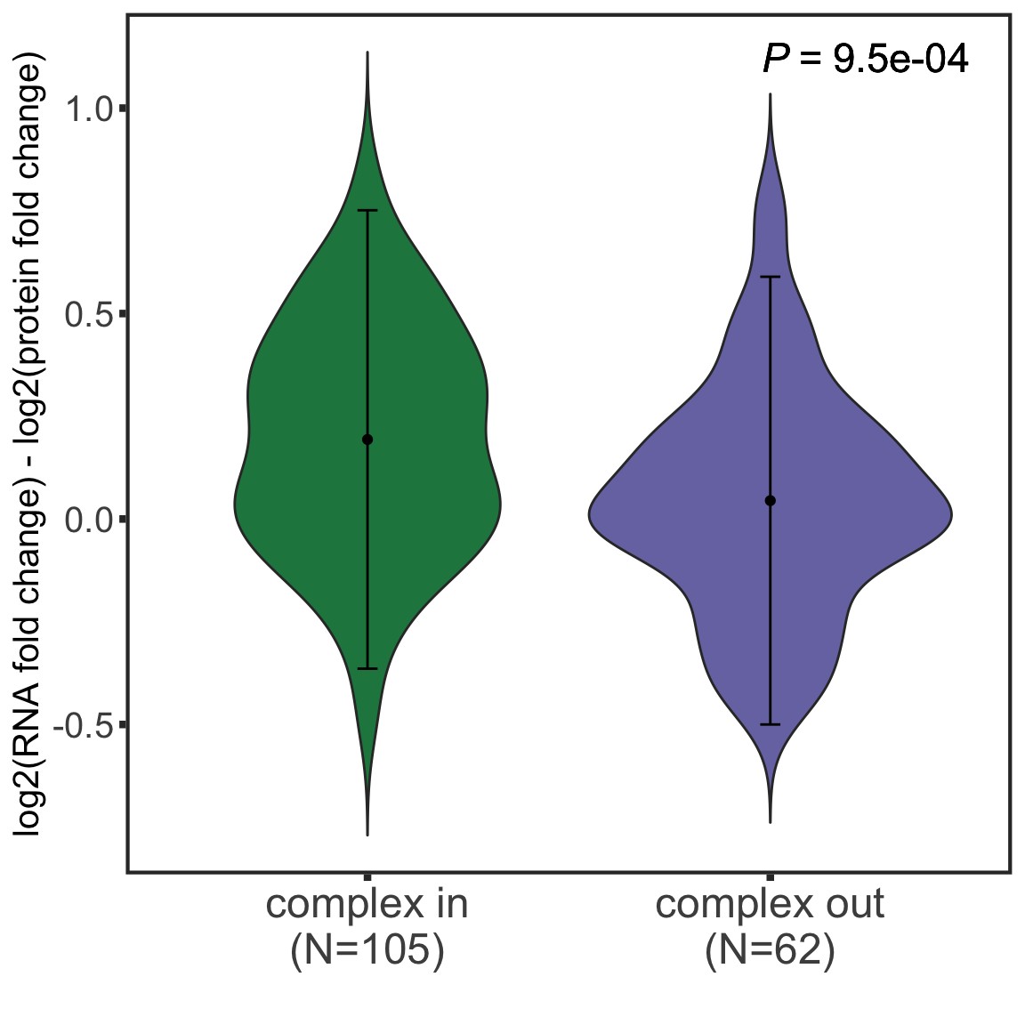
#ggsave("bufferComplexViolin.pdf", height = 6, width = 4.5)Construct protein-protein interaction network by connecting chr12 proteins and non-chr12 protein
comTab <- int_pairs %>% select(ProtA, ProtB, database) %>%
  mutate(chrA = rowData(protCLL[ProtA,])$chromosome_name,
         chrB = rowData(protCLL[ProtB,])$chromosome_name) %>%
  filter(!is.na(chrA), !is.na(chrB)) %>%
  filter((chrA == "12" & chrB != "12") | (chrA !="12" & chrB == "12")) %>%
  mutate(source = ifelse(chrA == 12, ProtA, ProtB),
         target = ifelse(chrA == 12, ProtB, ProtA)) %>%
  select(source, target, database)
fdrCut <- 0.05
resTab <- select(allRes, name, uniprotID, chrom, padj, padj.rna, log2FC,log2FC.rna) %>%
mutate(sigProt = padj <= fdrCut,
sigRna = padj.rna <=fdrCut,
upProt = sigProt & log2FC > 0,
upRna = sigRna & log2FC.rna > 0)
comTab <- comTab %>%
left_join(resTab, by = c(source = "uniprotID")) %>%
left_join(resTab, by = c(target = "uniprotID")) %>%
rename_all(funs(str_replace(., "x", "source"))) %>%
rename_all(funs(str_replace(., "y", "target"))) comTab.filter <- filter(comTab, upRna.source, upProt.source, upProt.target)#get node list
allNodes <- union(comTab.filter$name.source, comTab.filter$name.target)
nodeList <- data.frame(id = seq(length(allNodes))-1, name = allNodes, stringsAsFactors = FALSE) %>%
mutate(chromosome = ifelse(rowData(protCLL[match(name, rowData(protCLL)$hgnc_symbol),])$chromosome_name %in% "12",
"chr12","other"))
#get edge list
edgeList <- select(comTab.filter, name.source, name.target, database, upRna.target) %>%
dplyr::rename(Source = name.source, Target = name.target) %>%
mutate(Source = nodeList[match(Source,nodeList$name),]$id,
Target = nodeList[match(Target, nodeList$name),]$id,
sigRNA = ifelse(upRna.target,"yes","no")) %>%
data.frame(stringsAsFactors = FALSE)
net <- graph_from_data_frame(vertices = nodeList, d=edgeList, directed = FALSE)tidyNet <- as_tbl_graph(net)
complexNet <- ggraph(tidyNet, layout = "igraph", algorithm = "nicely") +
geom_edge_link(color = colList[3], width=1) +
geom_node_point(aes(color =chromosome, shape = chromosome), size=6) +
geom_node_text(aes(label = name), repel = TRUE, size=6) +
#scale_edge_linetype_manual(values = c(no = "dotted", yes = "solid"), name = "RNA up-regulated")+
scale_color_manual(values = c(chr12 = colList[1],other = colList[2])) +
scale_edge_color_brewer(palette = "Set2") +
theme_graph(base_family = "sans") + theme(legend.position = "bottom")
complexNet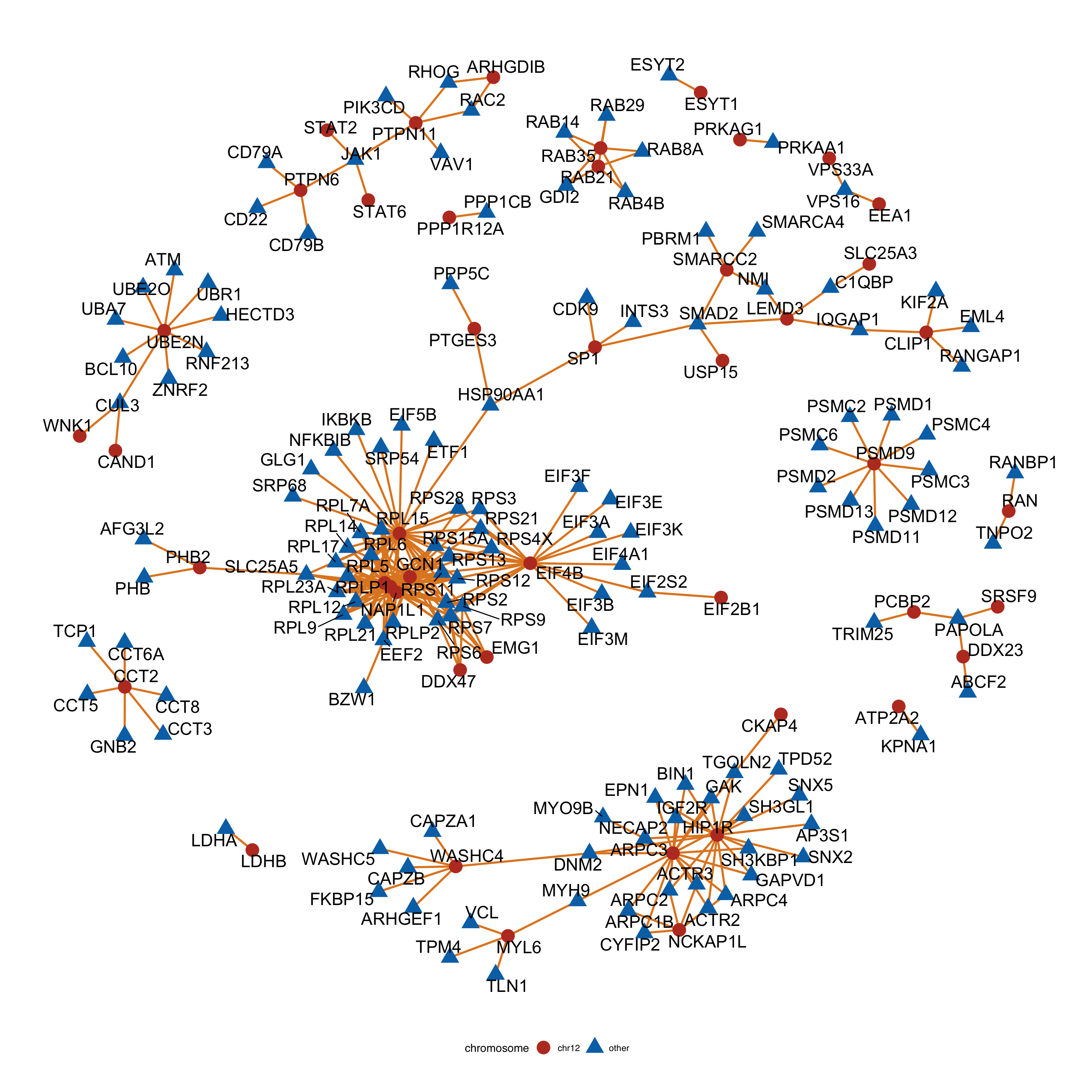
#ggsave("trisomy12Complex.pdf", height = 15, width = 15)Associate gene expression, protein expression and pathways on Chr12 and Chr19
load("../output/deResListRNA_allGene.RData")
load("../output/deResList.RData")
rnaRes <- resListRNA_allGene %>% filter(Gene == "trisomy12") %>%
  mutate(Chr = rowData(dds[id,])$chromosome) %>%
  filter(Chr == "12", adj.P.Val <= 0.05, t > 0) %>%
  distinct(name)

protRes <- resList %>% filter(Gene == "trisomy12") %>%
    mutate(Chr = rowData(protCLL[id,])$chromosome_name) %>%
    filter(Chr == "12", adj.P.Val <=0.05, t >0) %>%
    distinct(name)
Associations between PI3K/Akt/mTOR inhibitor responses and trisomy12
Prepare table
load("../data/screenData_enc.RData")
screenData <- screenData %>% filter(patientID %in% colnames(protCLL),
                                        Drug %in% c("Duvelisib","MK-2206","Rapamycin")) %>%
  group_by(patientID, Drug) %>% summarise(viab = mean(normVal.cor_auc)) %>%
  mutate(trisomy12 = patMeta[match(patientID, patMeta$Patient.ID),]$trisomy12,
         IGHV = patMeta[match(patientID, patMeta$Patient.ID),]$IGHV.status) %>%
  mutate(status = ifelse(trisomy12==1,"trisomy12","other"),
         IGHV = ifelse(IGHV=="M","M-CLL","U-CLL"),
         Drug = as.character(Drug))
Sample size
table(distinct(screenData, patientID, trisomy12)$trisomy12)
 0  1
59 23
T-test
All samples
tRes <- group_by(screenData, Drug) %>% nest() %>%
  mutate(m = map(data, ~t.test(viab~trisomy12,.))) %>%
  mutate(res = map(m, broom::tidy)) %>%
  unnest(res) %>%
  select(Drug, estimate, p.value)
tRes
# A tibble: 3 x 3
# Groups: Drug [3]
Drug estimate p.value
<chr> <dbl> <dbl>
1 Duvelisib 0.0787 0.0117
2 MK-2206 0.0324 0.00631
3 Rapamycin 0.0568 0.0139 IGHV stratified
tRes.ighv <- group_by(screenData, Drug, IGHV) %>% nest() %>%
  mutate(m = map(data, ~t.test(viab~trisomy12,.))) %>%
  mutate(res = map(m, broom::tidy)) %>%
  unnest(res) %>%
  select(Drug,IGHV, estimate, p.value)
tRes.ighv
# A tibble: 6 x 4
# Groups: Drug, IGHV [6]
Drug IGHV estimate p.value
<chr> <chr> <dbl> <dbl>
1 Duvelisib M-CLL 0.0438 0.340
2 MK-2206 M-CLL 0.0111 0.406
3 Rapamycin M-CLL 0.0507 0.217
4 Duvelisib U-CLL 0.103 0.000474
5 MK-2206 U-CLL 0.0517 0.00422
6 Rapamycin U-CLL 0.0637 0.0122 Visualization
All samples
Function for plot drug effect as boxplots
plotDrugBox <- function(screenData, tRes, y_lab = "Viability") {
  ymax <- max(screenData$viab)
  ymin <- min(screenData$viab)
  plotList <- lapply(unique(screenData$Drug), function(n) {
    eachTab <- filter(screenData, Drug == n) %>%
      group_by(status) %>% mutate(n=n()) %>% ungroup() %>%
      mutate(group = sprintf("%s\n(N=%s)",status,n)) %>%
      arrange(status) %>% mutate(group = factor(group, levels = unique(group)))

    pval <- formatNum(filter(tRes, Drug == n)$p.value, digits = 1, format="e")
    annoText <- bquote(.(n)~" ("~italic("P")~"="~.(pval)~")")


    ggplot(eachTab, aes(x=group, y = viab)) +
      geom_beeswarm(aes(col=IGHV), size =2.5,cex = 2, alpha=0.8) +
      geom_boxplot(fill = NA, width=0.3, outlier.shape = NA) +
      ggtitle(annoText)+
      #ggtitle(sprintf("%s (p = %s)",geneName, formatNum(pval, digits = 1, format = "e"))) +
      ylab(y_lab) + xlab("") +
      scale_color_manual(values = colList[2:3]) +
      scale_y_continuous(limits=c(ymin,ymax),labels = scales::number_format(accuracy = 0.1))+
      theme_full +
      theme(legend.position = "bottom",
            plot.title = element_text(hjust = 0.5),
            plot.margin = margin(0,20,0,20))

   })
  return(plotList)
}
All samples
pList <- plotDrugBox(screenData, tRes)
plot_grid(plotlist = pList, ncol=3)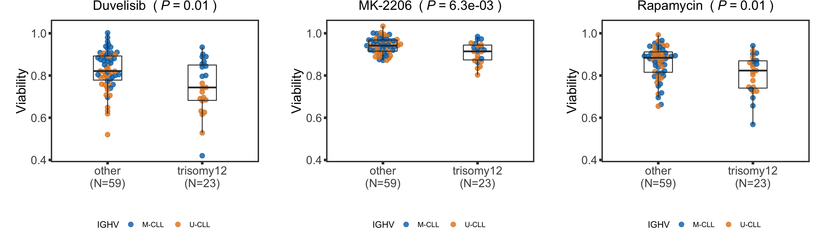
IGHV stratified
Function for plot drug effect as boxplots
plotDrugBoxIGHV <- function(screenData, tRes.ighv, y_lab = "Viability") {
  screenData <- mutate(screenData, drugIGHV =paste0(Drug,"_",IGHV))
  tRes.ighv <- mutate(tRes.ighv, drugIGHV = paste0(Drug, "_",IGHV))
  ymax <- max(screenData$viab)
  ymin <- min(screenData$viab)

  plotList <- lapply(unique(screenData$drugIGHV), function(n) {
    eachTab <- filter(screenData, drugIGHV == n) %>%
      group_by(status) %>% mutate(n=n()) %>% ungroup() %>%
      mutate(group = sprintf("%s\n(N=%s)",status,n)) %>%
      arrange(status) %>% mutate(group = factor(group, levels = unique(group)))
    drug <- unique(eachTab$Drug)
    ighv <- unique(eachTab$IGHV)
    pval <- formatNum(filter(tRes.ighv, drugIGHV == n)$p.value, digits = 1, format="e")
    annoText <- bquote(.(drug)~" ("~italic("P")~"="~.(pval)~","~.(ighv)~")")


    ggplot(eachTab, aes(x=group, y = viab)) +
      geom_beeswarm(aes(col=IGHV), size =2.5,cex = 2, alpha=0.8) +
      geom_boxplot(fill = NA, width=0.3, outlier.shape = NA) +
      ggtitle(annoText)+
      #ggtitle(sprintf("%s (p = %s)",geneName, formatNum(pval, digits = 1, format = "e"))) +
      ylab(y_lab) + xlab("") +
      scale_color_manual(values = c(`M-CLL` = colList[2], `U-CLL` = colList[3])) +
      scale_y_continuous(limits=c(ymin,ymax), labels = scales::number_format(accuracy = 0.1))+
      theme_full +
      theme(legend.position = "none",
            plot.title = element_text(hjust = 0.5),
            plot.margin = margin(20,20,20,20))

   })
  return(plotList)
}
pList <- plotDrugBoxIGHV(screenData, tRes.ighv)
plot_grid(plotlist = pList, ncol=3)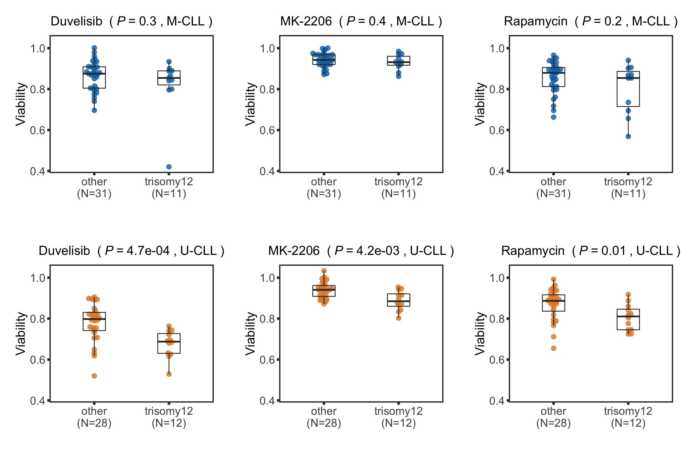
sessionInfo()R version 4.0.2 (2020-06-22)
Platform: x86_64-apple-darwin17.0 (64-bit)
Running under: macOS 10.16
Matrix products: default
BLAS: /Library/Frameworks/R.framework/Versions/4.0/Resources/lib/libRblas.dylib
LAPACK: /Library/Frameworks/R.framework/Versions/4.0/Resources/lib/libRlapack.dylib
locale:
[1] en_US.UTF-8/en_US.UTF-8/en_US.UTF-8/C/en_US.UTF-8/en_US.UTF-8
attached base packages:
[1] grid parallel stats4 stats graphics grDevices utils
[8] datasets methods base
other attached packages:
[1] circlize_0.4.12 piano_2.4.0
[3] latex2exp_0.4.0 forcats_0.5.1
[5] stringr_1.4.0 dplyr_1.0.5
[7] purrr_0.3.4 readr_1.4.0
[9] tidyr_1.1.3 tibble_3.1.0
[11] tidyverse_1.3.0 ggbeeswarm_0.6.0
[13] ComplexHeatmap_2.4.3 pheatmap_1.0.12
[15] proDA_1.2.0 ggraph_2.0.5
[17] ggplot2_3.3.3 igraph_1.2.6
[19] cowplot_1.1.1 tidygraph_1.2.0
[21] DESeq2_1.28.1 SummarizedExperiment_1.18.2
[23] DelayedArray_0.14.1 matrixStats_0.58.0
[25] Biobase_2.48.0 GenomicRanges_1.40.0
[27] GenomeInfoDb_1.24.2 IRanges_2.22.2
[29] S4Vectors_0.26.1 BiocGenerics_0.34.0
[31] limma_3.44.3
loaded via a namespace (and not attached):
[1] rappdirs_0.3.3 exactRankTests_0.8-31 bit64_4.0.5
[4] knitr_1.31 multcomp_1.4-16 data.table_1.14.0
[7] rpart_4.1-15 RCurl_1.98-1.2 generics_0.1.0
[10] TH.data_1.0-10 RSQLite_2.2.3 bit_4.0.4
[13] xml2_1.3.2 lubridate_1.7.10 httpuv_1.5.5
[16] assertthat_0.2.1 viridis_0.5.1 xfun_0.21
[19] hms_1.0.0 jquerylib_0.1.3 evaluate_0.14
[22] promises_1.2.0.1 fansi_0.4.2 progress_1.2.2
[25] caTools_1.18.1 dbplyr_2.1.0 readxl_1.3.1
[28] km.ci_0.5-2 DBI_1.1.1 geneplotter_1.66.0
[31] htmlwidgets_1.5.3 ellipsis_0.3.1 jyluMisc_0.1.5
[34] crosstalk_1.1.1 ggpubr_0.4.0 backports_1.2.1
[37] annotate_1.66.0 vctrs_0.3.6 abind_1.4-5
[40] cachem_1.0.4 withr_2.4.1 ggforce_0.3.3
[43] checkmate_2.0.0 prettyunits_1.1.1 cluster_2.1.1
[46] crayon_1.4.1 drc_3.0-1 relations_0.6-9
[49] genefilter_1.70.0 pkgconfig_2.0.3 slam_0.1-48
[52] labeling_0.4.2 tweenr_1.0.1 nlme_3.1-152
[55] vipor_0.4.5 nnet_7.3-15 rlang_0.4.10
[58] lifecycle_1.0.0 sandwich_3.0-0 BiocFileCache_1.12.1
[61] modelr_0.1.8 cellranger_1.1.0 rprojroot_2.0.2
[64] polyclip_1.10-0 Matrix_1.3-2 KMsurv_0.1-5
[67] carData_3.0-4 zoo_1.8-9 reprex_1.0.0
[70] base64enc_0.1-3 beeswarm_0.3.1 GlobalOptions_0.1.2
[73] png_0.1-7 viridisLite_0.3.0 rjson_0.2.20
[76] bitops_1.0-6 shinydashboard_0.7.1 KernSmooth_2.23-18
[79] visNetwork_2.0.9 blob_1.2.1 workflowr_1.6.2
[82] shape_1.4.5 maxstat_0.7-25 jpeg_0.1-8.1
[85] rstatix_0.7.0 ggsignif_0.6.1 scales_1.1.1
[88] memoise_2.0.0 magrittr_2.0.1 gplots_3.1.1
[91] zlibbioc_1.34.0 compiler_4.0.2 RColorBrewer_1.1-2
[94] plotrix_3.8-1 clue_0.3-58 cli_2.3.1
[97] XVector_0.28.0 htmlTable_2.1.0 Formula_1.2-4
[100] MASS_7.3-53.1 mgcv_1.8-34 tidyselect_1.1.0
[103] stringi_1.5.3 highr_0.8 yaml_2.2.1
[106] askpass_1.1 locfit_1.5-9.4 latticeExtra_0.6-29
[109] ggrepel_0.9.1 survMisc_0.5.5 sass_0.3.1
[112] fastmatch_1.1-0 tools_4.0.2 rio_0.5.26
[115] rstudioapi_0.13 foreign_0.8-81 git2r_0.28.0
[118] gridExtra_2.3 farver_2.1.0 digest_0.6.27
[121] shiny_1.6.0 Rcpp_1.0.6 car_3.0-10
[124] broom_0.7.5 later_1.1.0.1 httr_1.4.2
[127] survminer_0.4.9 AnnotationDbi_1.50.3 colorspace_2.0-0
[130] rvest_1.0.0 XML_3.99-0.5 fs_1.5.0
[133] splines_4.0.2 graphlayouts_0.7.1 xtable_1.8-4
[136] jsonlite_1.7.2 marray_1.66.0 R6_2.5.0
[139] sets_1.0-18 Hmisc_4.5-0 pillar_1.5.1
[142] htmltools_0.5.1.1 mime_0.10 glue_1.4.2
[145] fastmap_1.1.0 DT_0.17 BiocParallel_1.22.0
[148] codetools_0.2-18 fgsea_1.14.0 mvtnorm_1.1-1
[151] utf8_1.1.4 lattice_0.20-41 bslib_0.2.4
[154] curl_4.3 gtools_3.8.2 zip_2.1.1
[157] shinyjs_2.0.0 openxlsx_4.2.3 openssl_1.4.3
[160] survival_3.2-7 rmarkdown_2.7 munsell_0.5.0
[163] GetoptLong_1.0.5 GenomeInfoDbData_1.2.3 haven_2.3.1
[166] gtable_0.3.0