Section 8: Identifying protein biomarkers drug responses and clinical outcomes
Junyan Lu
2020-10-09
Last updated: 2021-05-06
Checks: 6 1
Knit directory: CLLproteomics_publish_revision/analysis/
This reproducible R Markdown analysis was created with workflowr (version 1.6.2). The Checks tab describes the reproducibility checks that were applied when the results were created. The Past versions tab lists the development history.
The R Markdown is untracked by Git. To know which version of the R Markdown file created these results, you’ll want to first commit it to the Git repo. If you’re still working on the analysis, you can ignore this warning. When you’re finished, you can run wflow_publish to commit the R Markdown file and build the HTML.
Great job! The global environment was empty. Objects defined in the global environment can affect the analysis in your R Markdown file in unknown ways. For reproduciblity it’s best to always run the code in an empty environment.
The command set.seed(20200227) was run prior to running the code in the R Markdown file. Setting a seed ensures that any results that rely on randomness, e.g. subsampling or permutations, are reproducible.
Great job! Recording the operating system, R version, and package versions is critical for reproducibility.
Nice! There were no cached chunks for this analysis, so you can be confident that you successfully produced the results during this run.
Great job! Using relative paths to the files within your workflowr project makes it easier to run your code on other machines.
Great! You are using Git for version control. Tracking code development and connecting the code version to the results is critical for reproducibility.
The results in this page were generated with repository version 3fb50c5. See the Past versions tab to see a history of the changes made to the R Markdown and HTML files.
Note that you need to be careful to ensure that all relevant files for the analysis have been committed to Git prior to generating the results (you can use wflow_publish or wflow_git_commit). workflowr only checks the R Markdown file, but you know if there are other scripts or data files that it depends on. Below is the status of the Git repository when the results were generated:
Ignored files:
    Ignored:    .DS_Store
    Ignored:    .Rhistory
    Ignored:    .Rproj.user/
    Ignored:    analysis/.DS_Store
    Ignored:    analysis/.Rhistory
    Ignored:    analysis/manuscript_S1_Overview_cache/
    Ignored:    analysis/manuscript_S2_genomicAssociation_cache/
    Ignored:    analysis/manuscript_S3_trisomy12_cache/
    Ignored:    analysis/manuscript_S4_IGHV_cache/
    Ignored:    analysis/manuscript_S5_trisomy19_cache/
    Ignored:    analysis/manuscript_S6_del11q_cache/
    Ignored:    code/.DS_Store
    Ignored:    code/.Rhistory
    Ignored:    data/.DS_Store
    Ignored:    output/.DS_Store

Untracked files:
    Untracked:  analysis/.trisomy12_norm.pdf
    Untracked:  analysis/IGHV_box.pdf
    Untracked:  analysis/IGHV_enrich.pdf
    Untracked:  analysis/IGHV_volcano.pdf
    Untracked:  analysis/bufferComplexViolin.pdf
    Untracked:  analysis/buffer_Tri12vsTri19.pdf
    Untracked:  analysis/cohortComposition_all.pdf
    Untracked:  analysis/drugBar.pdf
    Untracked:  analysis/dubelisib_tri12.pdf
    Untracked:  analysis/heatmap_tri12_circle.pdf
    Untracked:  analysis/manuscript_S1_Overview.Rmd
    Untracked:  analysis/manuscript_S2_genomicAssociation.Rmd
    Untracked:  analysis/manuscript_S3_trisomy12.Rmd
    Untracked:  analysis/manuscript_S4_IGHV.Rmd
    Untracked:  analysis/manuscript_S5_trisomy19.Rmd
    Untracked:  analysis/manuscript_S6_del11q.Rmd
    Untracked:  analysis/manuscript_S7_SF3B1.Rmd
    Untracked:  analysis/manuscript_S8_drugResponse_Outcomes.Rmd
    Untracked:  analysis/manuscript_S9_STAT2.Rmd
    Untracked:  analysis/plot_PC1_PC2.pdf
    Untracked:  analysis/protDrugTP53.pdf
    Untracked:  analysis/timsTOF_validate.Rmd
    Untracked:  analysis/tri12_transEnrich.pdf
    Untracked:  analysis/tri19_dosage_effect.pdf
    Untracked:  analysis/tri19_sum_buffer_number.pdf
    Untracked:  analysis/trisomy12_chr_summary.pdf
    Untracked:  code/utils.R
    Untracked:  data/Annotation file March 2021.xlsx
    Untracked:  data/CAS9results.xlsx
    Untracked:  data/CNV_onChrom.RData
    Untracked:  data/ComplexParticipantsPubMedIdentifiers_human.txt
    Untracked:  data/Fig1A.png
    Untracked:  data/IGLV321_SupplementalTables_R2.xlsx
    Untracked:  data/MOFAout.RData
    Untracked:  data/MOFAout_atLeast3.RData
    Untracked:  data/STATexprPCR.xlsx
    Untracked:  data/Western_blot_results_20210309_short.csv
    Untracked:  data/Western_blot_results_separate_blots.xlsx
    Untracked:  data/allComplexes.txt
    Untracked:  data/ddsrna_enc.RData
    Untracked:  data/exprCNV_enc.RData
    Untracked:  data/geneAnno.RData
    Untracked:  data/gmts/
    Untracked:  data/ic50.RData
    Untracked:  data/mofaIn.RData
    Untracked:  data/mofaIn_atLeast3.RData
    Untracked:  data/patMeta_enc.RData
    Untracked:  data/pepCLL_lumos_enc.RData
    Untracked:  data/protMOFA.RData
    Untracked:  data/proteins_in_complexes
    Untracked:  data/proteomic_LUMOS_2pep_enc.RData
    Untracked:  data/proteomic_explore_enc.RData
    Untracked:  data/proteomic_independent_all_enc.RData
    Untracked:  data/proteomic_independent_enc.RData
    Untracked:  data/proteomic_timsTOF_enc.RData
    Untracked:  data/screenData_enc.RData
    Untracked:  data/setToPathway.txt
    Untracked:  data/survival_enc.RData
    Untracked:  output/MSH6_splicing.svg
    Untracked:  output/SUGP1_splicing.svg
    Untracked:  output/deResList.RData
    Untracked:  output/deResListBatch2.RData
    Untracked:  output/deResListRNA.RData
    Untracked:  output/deResListRNA_allGene.RData
    Untracked:  output/deResList_WBC.RData
    Untracked:  output/deResList_batch1.RData
    Untracked:  output/deResList_batch3.RData
    Untracked:  output/deResList_independent.RData
    Untracked:  output/deResList_timsTOF.RData
    Untracked:  output/dxdCLL.RData
    Untracked:  output/dxdCLL2.RData
    Untracked:  output/exprCNV.RData
    Untracked:  output/geneAnno.RData
    Untracked:  output/int_pairs.csv
    Untracked:  output/lassoResults_CPS.RData
    Untracked:  output/resOutcome_batch1.RData
    Untracked:  output/resOutcome_batch13.RData
    Untracked:  output/resOutcome_batch2.RData
    Untracked:  output/resOutcome_batch3.RData

Unstaged changes:
    Modified:   analysis/_site.yml
    Deleted:    analysis/analysisSF3B1.Rmd
    Deleted:    analysis/comparePlatforms.Rmd
    Deleted:    analysis/compareProteomicsRNAseq.Rmd
    Deleted:    analysis/correlateCLLPD.Rmd
    Deleted:    analysis/correlateGenomic.Rmd
    Deleted:    analysis/correlateGenomic_removePC.Rmd
    Deleted:    analysis/correlateMIR.Rmd
    Deleted:    analysis/correlateMethylationCluster.Rmd
    Modified:   analysis/index.Rmd
    Deleted:    analysis/predictOutcome.Rmd
    Deleted:    analysis/processProteomics_LUMOS.Rmd
    Deleted:    analysis/processProteomics_timsTOF.Rmd
    Deleted:    analysis/qualityControl_LUMOS.Rmd
    Deleted:    analysis/qualityControl_timsTOF.Rmd
Note that any generated files, e.g. HTML, png, CSS, etc., are not included in this status report because it is ok for generated content to have uncommitted changes.
There are no past versions. Publish this analysis with wflow_publish() to start tracking its development.
Load packages and datasets
knitr::opts_chunk$set(echo = TRUE, warning = FALSE, message = FALSE, dev = c("png","pdf"))
library(limma)
library(pheatmap)
library(jyluMisc)
library(survival)
library(survminer)
library(maxstat)
library(igraph)
library(tidygraph)
library(ggraph)
library(glmnet)
library(SummarizedExperiment)
library(cowplot)
library(tidyverse)

load("../data/patMeta_enc.RData")
load("../data/ddsrna_enc.RData")
load("../data/proteomic_explore_enc.RData")
load("../output/deResList.RData") #precalculated differential expression
load("../data/survival_enc.RData")
load("../data/screenData_enc.RData")

#protCLL <- protCLL[rowData(protCLL)$uniqueMap,]
source("../code/utils.R")
Correlations between protein abundance and drug response
Preprocess datasets
Drug screening data from 1000CPS: low quality samples after QC are removed; the edge effect corrected viability values are used
viabMat <- screenData %>% filter(!lowQuality, ! Drug %in% c("DMSO","PBS"), patientID %in% colnames(protCLL)) %>%
  group_by(patientID, Drug) %>% summarise(viab = mean(normVal.adj.cor_auc)) %>%
  spread(key = patientID, value = viab) %>%
  data.frame(stringsAsFactors = FALSE) %>% column_to_rownames("Drug") %>%
  as.matrix()
Proteomics data
proMat <- assays(protCLL)[["count"]]
proMat <- proMat[,colnames(viabMat)]

#Remove proteins without much variance (to lower multi-testing burden)

#sds <- genefilter::rowSds(proMat,na.rm=TRUE)
#proMat <- proMat[sds > genefilter::shorth(sds),]
How many samples have both proteomics data and CPS1000 screen data
ncol(proMat)[1] 82Association test using univariate test
resTab.auc <- lapply(rownames(viabMat),function(drugName) {
  viab <- viabMat[drugName, ]
  batch <- protCLL[,colnames(viabMat)]$batch
  designMat <- model.matrix(~1+viab+batch)
  fit <- lmFit(proMat,  designMat)
  fit2 <- eBayes(fit)
  corRes <- topTable(fit2, number ="all", adjust.method = "BH", coef = "viab") %>% rownames_to_column("id") %>%
    mutate(symbol = rowData(protCLL[id,])$hgnc_symbol, Drug = drugName) %>%
    mutate(adj.P.Val = p.adjust(P.Value, method = "BH"))
}) %>% bind_rows() %>% arrange(P.Value)
Bar plot to show the number of significant associations (5% FDR)
#Select significant associations (10% FDR)
resTab.sig <- filter(resTab.auc, adj.P.Val <= 0.05) %>%
  select(Drug, symbol, id,logFC, P.Value, adj.P.Val)

plotTab <- resTab.sig %>%
  group_by(Drug) %>%
  summarise(n = length(id)) %>% ungroup()
ordTab <- group_by(plotTab, Drug) %>% summarise(total = sum(n)) %>%
  arrange(desc(total))
plotTab <- mutate(plotTab, Drug = factor(Drug, levels = ordTab$Drug)) %>%
  filter(n>0)

drugBar <- ggplot(plotTab, aes(x=Drug, y = n)) + geom_bar(stat="identity",fill=colList[4]) +
  geom_text(aes(label = paste0(n)),vjust=-1,col="black", size=6) +
  ylim(0,500)+ #annotate("text", label = "Number of associations (10% FDR)", x=Inf, y=Inf,hjust=1, vjust=1, size=6)+
  theme_half + theme(axis.text.x = element_text(angle = 90, hjust=1, vjust=0.5)) +
  ylab("Number of associations (5% FDR)") + xlab("")
Table of significant associations (5% FDR)
resTab.sig %>% mutate_if(is.numeric, formatC, digits=2, format= "e") %>%
  DT::datatable()
Correlation plot of selected protein-drug pairs
Stratified by IGHV and trisomy12
proMat.combat <- assays(protCLL)[["count_combat"]]
proMat.combat <- proMat.combat[,colnames(viabMat)]

pairList <- list(c("Cobimetinib","STAT2"),c("Trametinib", "PTPN11"), c("Ibrutinib","LYN"),c("Ibrutinib","ANXA2"))
plotList <- lapply(pairList, function(pair) {
  textCol <- "darkred"
  drugName <- pair[1]
  proteinName <- pair[2]
  id <- rownames(protCLL)[match(proteinName, rowData(protCLL)$hgnc_symbol)]
  plotTab <- tibble(patID = colnames(viabMat),
                    viab = viabMat[drugName,],
                    expr = proMat.combat[id,]) %>%
    mutate(IGHV = protCLL[,patID]$IGHV.status,
           trisomy12 = protCLL[,patID]$trisomy12) %>%
    mutate(trisomy12 = ifelse(trisomy12 ==1,"yes","no")) %>%
    filter(!is.na(viab),!is.na(expr))

  pval <- formatNum(filter(resTab.sig, Drug == drugName, symbol == proteinName)$P.Value, digits = 1, format = "e")
  Rval <- sprintf("%1.2f",cor(plotTab$viab, plotTab$expr))
  Nval <- nrow(plotTab)
  annoP <- bquote(italic("P")~"="~.(pval))
  annoN <- bquote(N~"="~.(Nval))
  annoCoef <- bquote(R~"="~.(Rval))

  corPlot <- ggplot(plotTab, aes(x = viab, y = expr)) +
    geom_point(aes(col = trisomy12, shape = IGHV), size=5) +
    scale_shape_manual(values = c(M = 19, U = 1)) +
    scale_color_manual(values = c(yes = colList[2], no = colList[3])) +
    geom_smooth(formula = y~x,method = "lm", se=FALSE, color = "grey50", linetype ="dashed" ) +
    ggtitle(sprintf("%s ~ %s", drugName, proteinName)) +
    ylab("Protein expression") + xlab("Viability after treatment") +
    theme_full +
    theme(legend.position = "bottom")

  if (Rval < 0) annoPos <- "right" else annoPos <- "left"

  if (annoPos == "right") {

    corPlot <- corPlot + annotate("text", x = max(plotTab$viab), y = Inf, label = annoN,
                                  hjust=1, vjust =2, size = 5, parse = FALSE, col= textCol) +
      annotate("text", x = max(plotTab$viab), y = Inf, label = annoP,
               hjust=1, vjust =4, size = 5, parse = FALSE, col= textCol) +
      annotate("text", x = max(plotTab$viab), y = Inf, label = annoCoef,
               hjust=1, vjust =6, size = 5, parse = FALSE, col= textCol)

  } else if (annoPos== "left") {
    corPlot <- corPlot + annotate("text", x = min(plotTab$viab), y = Inf, label = annoN,
                                  hjust=0, vjust =2, size = 5, parse = FALSE, col= textCol) +
      annotate("text", x = min(plotTab$viab), y = Inf, label = annoP,
               hjust=0, vjust =4, size = 5, parse = FALSE, col= textCol) +
      annotate("text", x = min(plotTab$viab), y = Inf, label = annoCoef,
               hjust=0, vjust =6, size = 5, parse = FALSE, col= textCol)
  }

  corPlot <- corPlot + ylab("Protein expression") + xlab("Viability after treatment") +
    scale_y_continuous(labels = scales::number_format(accuracy = 0.1)) +
    scale_x_continuous(labels = scales::number_format(accuracy = 0.1))

  corPlot
})


drugCor <- cowplot::plot_grid(plotlist = plotList, ncol =2)
drugCor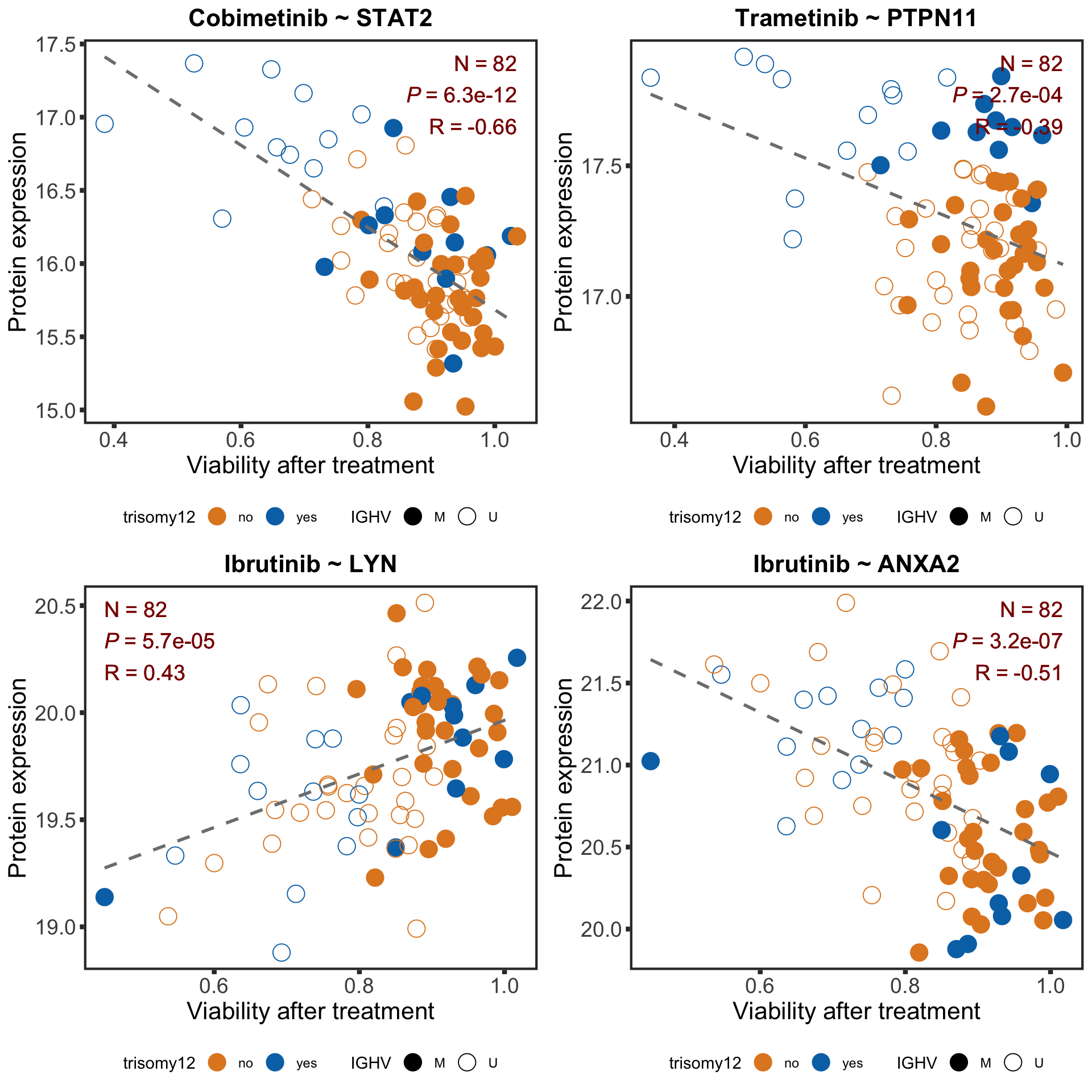
For TP53-MDM2 inhibitors, color the samples by their TP53 mutational status
pairListTP53 <- list(c("Nutlin-3a","USP5"),c("RO5963", "PHF23"))

plotList <- lapply(pairListTP53, function(pair) {
  textCol <- "darkred"
  drugName <- pair[1]
  proteinName <- pair[2]
  id <- rownames(protCLL)[match(proteinName, rowData(protCLL)$hgnc_symbol)]
  plotTab <- tibble(patID = colnames(viabMat),
                    viab = viabMat[drugName,],
                    expr = proMat.combat[id,]) %>%
    mutate(IGHV = protCLL[,patID]$IGHV.status,
           #trisomy12 = protCLL[,patID]$trisomy12,
           TP53 = patMeta[match(patID, patMeta$Patient.ID),]$TP53) %>%
    #mutate(trisomy12 = ifelse(trisomy12 ==1,"yes","no")) %>%
    mutate(TP53 = ifelse(TP53 ==1,"Mut","WT")) %>%
    filter(!is.na(viab),!is.na(expr))

  pval <- formatNum(filter(resTab.sig, Drug == drugName, symbol == proteinName)$P.Value, digits = 1, format = "e")
  Rval <- sprintf("%1.2f",cor(plotTab$viab, plotTab$expr))
  Nval <- nrow(plotTab)
  annoP <- bquote(italic("P")~"="~.(pval))
  annoN <- bquote(N~"="~.(Nval))
  annoCoef <- bquote(R~"="~.(Rval))

  corPlot <- ggplot(plotTab, aes(x = viab, y = expr)) +
    geom_point(aes(col = TP53, shape = IGHV), size=5) +
    scale_shape_manual(values = c(M = 19, U = 1)) +
    scale_color_manual(values = c(Mut = colList[2], WT = colList[3])) +
    geom_smooth(formula = y~x,method = "lm", se=FALSE, color = "grey50", linetype ="dashed" ) +
    ggtitle(sprintf("%s ~ %s", drugName, proteinName)) +
    ylab("Protein expression") + xlab("Viability after treatment") +
    theme_full +
    theme(legend.position = "bottom")

  if (Rval < 0) annoPos <- "right" else annoPos <- "left"

  if (annoPos == "right") {

    corPlot <- corPlot + annotate("text", x = max(plotTab$viab), y = Inf, label = annoN,
                                  hjust=1, vjust =2, size = 5, parse = FALSE, col= textCol) +
      annotate("text", x = max(plotTab$viab), y = Inf, label = annoP,
               hjust=1, vjust =4, size = 5, parse = FALSE, col= textCol) +
      annotate("text", x = max(plotTab$viab), y = Inf, label = annoCoef,
               hjust=1, vjust =6, size = 5, parse = FALSE, col= textCol)

  } else if (annoPos== "left") {
    corPlot <- corPlot + annotate("text", x = min(plotTab$viab), y = Inf, label = annoN,
                                  hjust=0, vjust =2, size = 5, parse = FALSE, col= textCol) +
      annotate("text", x = min(plotTab$viab), y = Inf, label = annoP,
               hjust=0, vjust =4, size = 5, parse = FALSE, col= textCol) +
      annotate("text", x = min(plotTab$viab), y = Inf, label = annoCoef,
               hjust=0, vjust =6, size = 5, parse = FALSE, col= textCol)
  }

  corPlot <- corPlot + ylab("Protein expression") + xlab("Viability after treatment") +
    scale_y_continuous(labels = scales::number_format(accuracy = 0.1)) +
    scale_x_continuous(labels = scales::number_format(accuracy = 0.1))

  corPlot
})


drugCorTP53 <- cowplot::plot_grid(plotlist = plotList, ncol =2)
drugCorTP53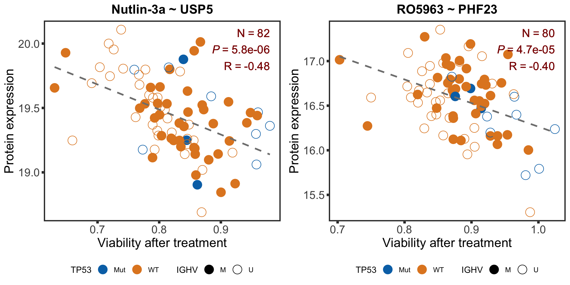
ggsave("protDrugTP53.pdf",height = 5, width = 10)Association test with blocking for IGHV and trisomy12
testList <- filter(resTab.auc, adj.P.Val <= 0.05)
resTab.auc.block <- lapply(seq(nrow(testList)),function(i) {
  pair <- testList[i,]
  expr <- proMat[pair$id,]
  viab <- viabMat[pair$Drug, ]
  ighv <- protCLL[,colnames(viabMat)]$IGHV.status
  tri12 <- protCLL[,colnames(viabMat)]$trisomy12
  batch <- protCLL[,colnames(viabMat)]$batch
  res <- anova(lm(viab~ighv+tri12+batch+expr))
  data.frame(id = pair$id, P.Value = res["expr",]$`Pr(>F)`, symbol = pair$symbol,
             Drug = pair$Drug,
             P.Value.IGHV = res["ighv",]$`Pr(>F)`,P.Value.trisomy12 = res["tri12",]$`Pr(>F)`,
             P.Value.noBlock = pair$P.Value,
             stringsAsFactors = FALSE)

}) %>% bind_rows() %>% mutate(adj.P.Val = p.adjust(P.Value, method = "BH")) %>% arrange(P.Value)
Assocations that are still significant
resList.sig.block <- filter(resTab.auc.block, adj.P.Val <= 0.05)
resList.sig.block %>% mutate_if(is.numeric, formatC, digits=2, format= "e") %>%
  DT::datatable()
The above mentioned pairs are still significant, indicate IGHV and trisomy12 independent assocations.
Barplot to show significant associations (5% FDR)
plotTab <- resList.sig.block %>% group_by(Drug) %>%
  summarise(n = length(id)) %>% ungroup()
ordTab <- group_by(plotTab, Drug) %>% summarise(total = sum(n)) %>%
  arrange(desc(total))
plotTab <- mutate(plotTab, Drug = factor(Drug, levels = ordTab$Drug)) %>%
  filter(n>0)

drugBar <- ggplot(plotTab, aes(x=Drug, y = n)) + geom_bar(stat="identity",fill=colList[4]) +
  geom_text(aes(label = paste0(n)),vjust=-1,col="black", size=6) +
  ylim(0,200)+ #annotate("text", label = "Number of associations (10% FDR)", x=Inf, y=Inf,hjust=1, vjust=1, size=6)+
  theme_half + theme(axis.text.x = element_text(angle = 90, hjust=1, vjust=0.5)) +
  ylab("Number of associations (5% FDR)") + xlab("")
Network plots to show significant associations (1% FDR)
1% FDR cut-off is chosen here for better visualization
dirTab <- select(resTab.sig, Drug, symbol, logFC) %>%
  mutate(correlation = ifelse(logFC>0,"positive","negative"))

comTab <- resList.sig.block %>%
  filter(adj.P.Val < 0.01) %>%
  select(symbol, Drug, adj.P.Val) %>%
  left_join(dirTab, by = c("Drug","symbol")) %>%
  mutate(source = symbol,
         target = Drug) %>%
  select(source, target, adj.P.Val, correlation)
#get node list
allNodes <- union(comTab$source, comTab$target)
nodeList <- data.frame(id = seq(length(allNodes))-1, name = allNodes, stringsAsFactors = FALSE) %>%
mutate(type = ifelse(name %in% comTab$source,"protein","drug"),
font = ifelse(name %in% comTab$source,"plain","bold"))
#get edge list
edgeList <- comTab %>%
dplyr::rename(Source = source, Target = target) %>%
mutate(Source = nodeList[match(Source,nodeList$name),]$id,
Target = nodeList[match(Target, nodeList$name),]$id) %>%
data.frame(stringsAsFactors = FALSE)
net <- graph_from_data_frame(vertices = nodeList, d=edgeList, directed = FALSE)tidyNet <- as_tbl_graph(net)
drugNet <- ggraph(tidyNet, layout = "igraph", algorithm = "fr") +
geom_edge_link(aes(color = correlation), width=1.5, edge_alpha=0.5) +
geom_node_point(aes(color = type, size = type)) +
geom_node_text(aes(label = name, fontface = font ), repel = FALSE, size=5) +
scale_size_manual(values = c(protein = 0, drug=25)) +
scale_color_manual(values = c(protein = colList[2],drug = "#D2FAD4")) +
scale_edge_color_manual(values = c("positive" = colList[1], "negative" = colList[2])) +
theme_graph(base_family = "sans") +
theme(legend.position = "bottom")
drugNet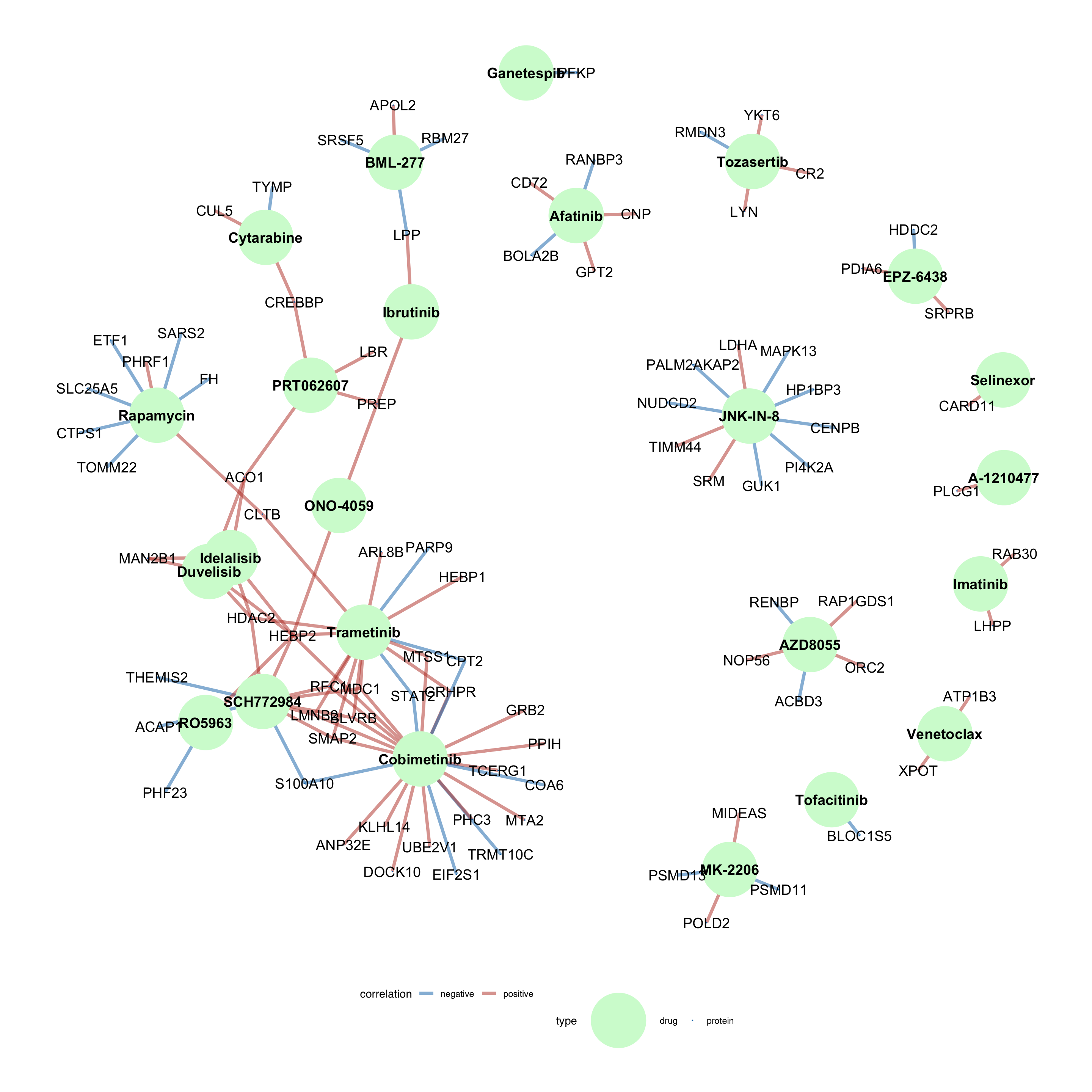
Using multi-variate model to test whether the protein expression can explain additional variance in drug response compared to genetic alone**
Prepare genomic annotations
geneMat <-  patMeta[match(colnames(proMat), patMeta$Patient.ID),] %>%
  select(Patient.ID, IGHV.status, del11q:U1) %>%
  mutate_if(is.factor, as.character) %>% mutate(IGHV.status = ifelse(IGHV.status == "M", 1,0)) %>%
  mutate_at(vars(-Patient.ID), as.numeric) %>% #assign a few unknown mutated cases to wildtype
  mutate_all(replace_na,0) %>%
  data.frame() %>% column_to_rownames("Patient.ID")


geneMat <- geneMat[,apply(geneMat,2, function(x) sum(x %in% 1, na.rm = TRUE))>=5] %>% as.matrix()
Genes that will be included in the multivariate model
colnames(geneMat) [1] "IGHV.status" "del11q" "del13q" "del17p" "trisomy12"
[6] "trisomy19" "NOTCH1" "ATM" "BRAF" "DDX3X"
[11] "EGR2" "SF3B1" "TP53" compareR2 <- function(Drug, protName, geneMat) {
viab <- viabMat[Drug,]
protID <- unique(filter(resTab.sig, symbol == protName)$id)
expr <- proMat[protID,]
tabGene <- data.frame(geneMat)
tabGene[["viab"]] <- viab
tabCom <- tabGene
tabCom[[protName]] <- expr
r2Prot <- summary(lm(viab~expr))$r.squared
r2Gene <- summary(lm(viab~., data=tabGene))$r.squared
r2Com <- summary(lm(viab~., data=tabCom))$r.squared
plotTab <- tibble(model = c(paste0(protName, " expression"), "genetics",sprintf("genetics + \n%s expression",protName)),
R2 = c(r2Prot, r2Gene, r2Com)) %>%
mutate(model= factor(model, levels = rev(model)))
ggplot(plotTab, aes(x=model, y = R2)) + geom_bar(aes(fill = model),stat="identity", width=0.6) + coord_flip() +
ggtitle(Drug) + ylab(bquote("Variance explained ("*R^2*")")) + xlab("") + ylim(0,0.7) +
scale_fill_manual(values = colList[4:6]) + theme_full +theme(legend.position = "none")
}plotList <- lapply(pairList, function(p) {
compareR2(p[1],p[2],geneMat)
})
#plotList[[1]] <- plotList[[1]] +ylab("")
plot_grid(plotlist= plotList, ncol= 1, align = "hv")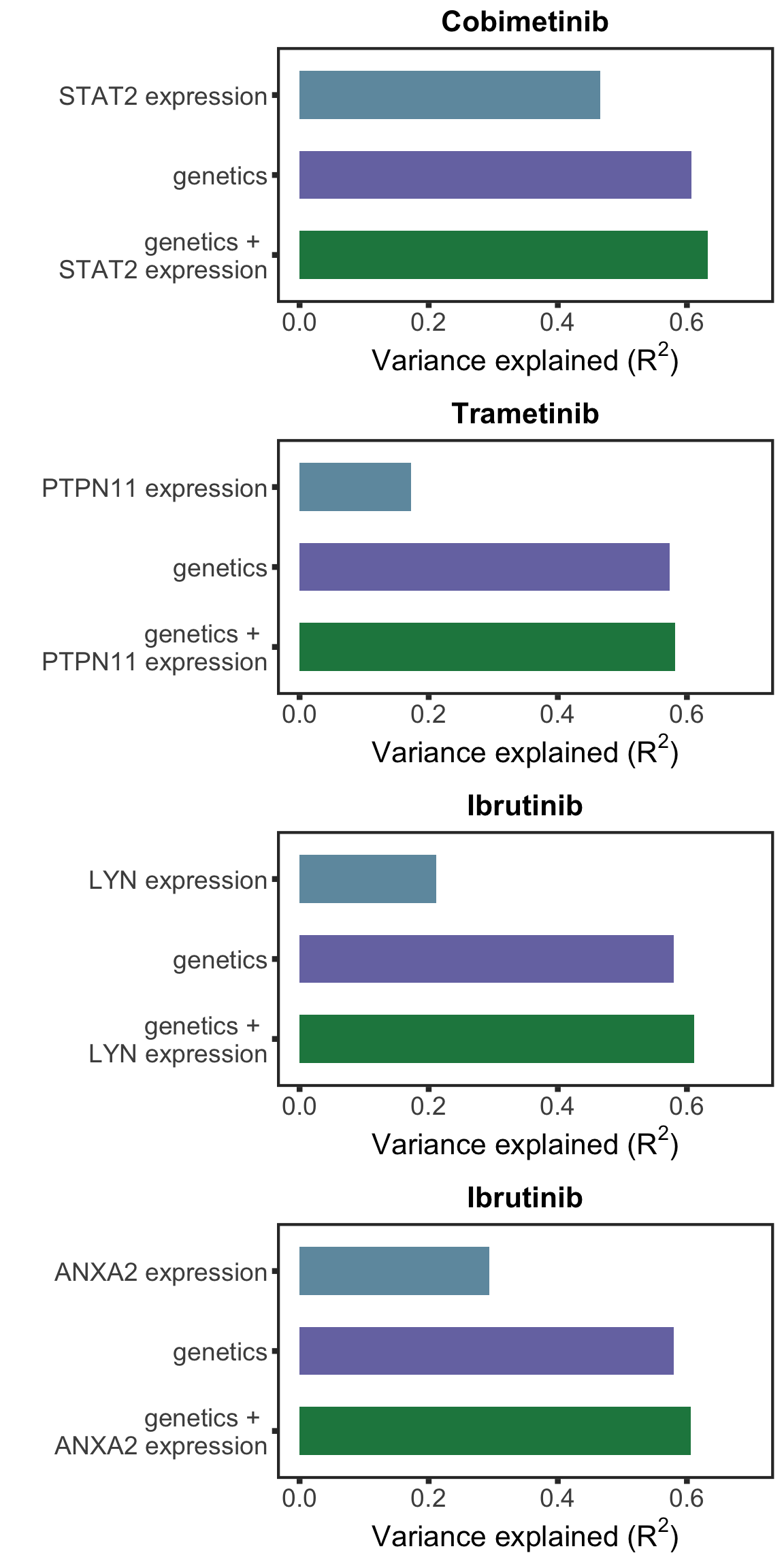
#ggsave("drugVarExp.pdf", height = 12, width = 6)plotListTP53 <- lapply(pairListTP53, function(p) {
compareR2(p[1],p[2],geneMat)
})
#plotList[[1]] <- plotList[[1]] +ylab("")
plot_grid(plotlist= plotListTP53, ncol= 1, align = "hv")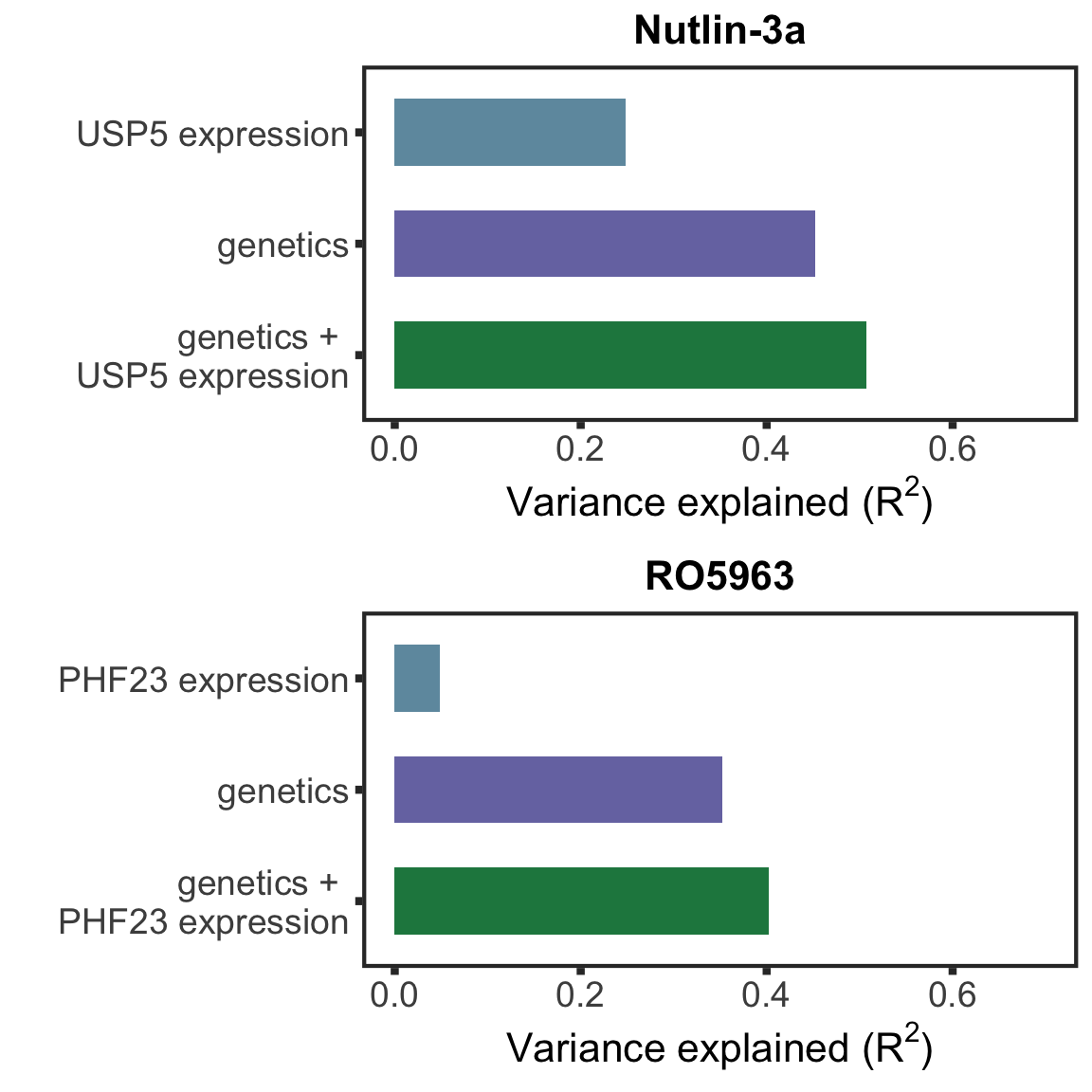
#ggsave("drugVarExpTP53.pdf", height = 6, width = 6)Protein markers for clincial outcomes
Uni-variate model to identify proteins associated with outcomes
protCLL.sub <- protCLL[!rowData(protCLL)$chromosome_name %in% c("X","Y"),]
protMat <- assays(protCLL.sub)[["count_combat"]]


survTab <- survT %>%
  select(patID, OS, died, TTT, treatedAfter, age,sex) %>%
  dplyr::rename(patientID = patID) %>%
  filter(patientID %in% colnames(protMat))
TTT events
table(survTab$treatedAfter)
FALSE  TRUE
   44    46
OS events
table(survTab$died)
FALSE  TRUE
   80    11
uniRes.ttt <- lapply(rownames(protMat), function(n) {
testTab <- mutate(survTab, expr = protMat[n, patientID])
com(testTab$expr, testTab$TTT, testTab$treatedAfter, TRUE) %>%
mutate(id = n)
}) %>% bind_rows() %>% mutate(p.adj = p.adjust(p, method = "BH")) %>%
arrange(p) %>% mutate(name = rowData(protCLL[id,])$hgnc_symbol) %>%
mutate(outcome = "TTT")
uniRes.os <- lapply(rownames(protMat), function(n) {
testTab <- mutate(survTab, expr = protMat[n, patientID])
com(testTab$expr, testTab$OS, testTab$died, TRUE) %>%
mutate(id = n)
}) %>% bind_rows() %>% mutate(p.adj = p.adjust(p, method = "BH")) %>%
arrange(p) %>% mutate(name = rowData(protCLL[id,])$hgnc_symbol) %>%
mutate(outcome = "OS")
uniRes <- bind_rows(uniRes.ttt, uniRes.os) %>%
mutate(p.adj = p.adjust(p, method = "BH"))A table showing significant associations
uniRes %>% filter(p.adj <= 0.05) %>% mutate_if(is.numeric, formatC, digits=2,format="e") %>%
  select(name, p, HR, p.adj, outcome) %>% DT::datatable()
Selecting protein markers independent of known risks using multi-vairate model
Prepare data
#table of known risks
riskTab <- select(survTab, patientID, age, sex) %>%
  left_join(patMeta[,c("Patient.ID","IGHV.status","TP53","trisomy12","del17p")], by = c(patientID = "Patient.ID")) %>%
  mutate(TP53 = as.numeric(as.character(TP53)),
         del17p = as.numeric(as.character(del17p))) %>%
  mutate(`TP53.del17p` = as.numeric(TP53 | del17p),
         IGHV = factor(ifelse(IGHV.status %in% "U",1,0))) %>%
  select(-TP53, -del17p,-IGHV.status) %>%
  mutate(age = age/10)
Multi-variate test
cTab.ttt <- lapply(filter(uniRes, outcome == "TTT", p.adj <=0.1)$id, function(n) {
  risk0 <- riskTab
  expr <- protMat[n,]
  expr <- (expr - mean(expr,na.rm=TRUE))/sd(expr,na.rm = TRUE)
  risk1 <- riskTab %>% mutate(protExpr = expr[patientID])
  res0 <- summary(runCox(survTab, risk0, "TTT","treatedAfter"))
  fullModel <- runCox(survTab, risk1, "TTT","treatedAfter")
  res1 <- summary(fullModel)
  tibble(id = n, c0 = res0$concordance[1], c1 = res1$concordance[1],
         se0 = res0$concordance[2],se1 = res1$concordance[2],
         ci0 = se0*1.96, ci1 = se1*1.96,
         p = res1$coefficients["protExpr",5],
         fullModel = list(fullModel))
}) %>% bind_rows() %>% mutate(diffC = c1-c0) %>%
  arrange(desc(diffC)) %>%
  mutate(name=rowData(protCLL[id,])$hgnc_symbol,
         outcome = "TTT")

cTab.os <- lapply(filter(uniRes, outcome == "OS", p.adj<=0.1)$id, function(n) {
  risk0 <- riskTab
  expr <- protMat[n,]
  expr <- (expr - mean(expr,na.rm=TRUE))/sd(expr,na.rm = TRUE)
  risk1 <- riskTab %>% mutate(protExpr = expr[patientID])
  res0 <- summary(runCox(survTab, risk0, "OS","died"))
  fullModel <- runCox(survTab, risk1, "OS","died")
  res1 <- summary(fullModel)

  tibble(id = n, c0 = res0$concordance[1], c1 = res1$concordance[1],
         se0 = res0$concordance[2],se1 = res1$concordance[2],
         ci0 = se0*1.96, ci1 = se1*1.96,
         p = res1$coefficients["protExpr",5],
         fullModel = list(fullModel))
}) %>% bind_rows() %>% mutate(diffC = c1-c0) %>%
  arrange(desc(diffC)) %>%
  mutate(name=rowData(protCLL[id,])$hgnc_symbol,
         outcome = "OS")

cTab <- bind_rows(cTab.ttt, cTab.os) %>%
  mutate(p.adj = p.adjust(p, method = "BH")) %>%
  arrange(p)
A table showing idependent protein markers
cTab %>% filter(p.adj <= 0.05) %>% mutate_if(is.numeric, formatC, digits=2,format="e") %>%
  select(name, p, p.adj, outcome) %>% DT::datatable()
Forest plot of several markers as examples
plotHazard <- function(survRes, protName, title = "", xLim = c(0.2,6)) {
  sumTab <- summary(survRes)$coefficients
  confTab <- summary(survRes)$conf.int
  #correct feature name
  nameOri <- rownames(sumTab)
  nameMod <- substr(nameOri, 1, nchar(nameOri) -1)
  plotTab <- tibble(feature = rownames(sumTab),
                    nameMod = substr(nameOri, 1, nchar(nameOri) -1),
                    HR = sumTab[,2],
                    p = sumTab[,5],
                    Upper = confTab[,4],
                    Lower = confTab[,3]) %>%
    mutate(feature = ifelse(nameMod %in% names(survRes$xlevels), nameMod, feature)) %>%
    mutate(feature = str_replace(feature, "[.]","/")) %>%
    mutate(feature = str_replace(feature, "[_]","-")) %>%
    mutate(feature = str_replace(feature, "IGHV","IGHV-U")) %>%
    mutate(candidate = ifelse(feature == "protExpr", "yes","no")) %>%
    mutate(feature = ifelse(feature == "protExpr", protName, feature)) %>%
    #arrange(desc(abs(p))) %>%
    mutate(feature = factor(feature, levels = feature)) #%>%
    #mutate(type = ifelse(HR >1 ,"up","down")) %>%
   # mutate(Upper = ifelse(Upper > 10, 10, Upper))

  p <- ggplot(plotTab, aes(x=feature, y = HR, color = candidate)) +
    geom_hline(yintercept = 1, linetype = "dotted") +
    geom_point(position = position_dodge(width=0.8), size=3) +
    geom_errorbar(aes(ymin = Lower, ymax = Upper), width = 0.3, size=1) +
    geom_text(position = position_nudge(x = 0.3),
              aes(y = HR, label =  sprintf("italic(P)~'='~'%s'",
                                           formatNum(p, digits = 1))),
              color = "black", size =5, parse = TRUE) +
    scale_color_manual(values = c(yes = "darkred", no = "black")) +
    ggtitle(title) + scale_y_log10(limits = xLim) +
    ylab("Hazard ratio") +
    coord_flip() +
    theme_full +
    theme(legend.position = "none", axis.title.y = element_blank())
  return(p)
}
NFKB2
protName <- "NFKB2"
outcomeName <- "TTT"
survRes <- filter(cTab, outcome == outcomeName , name == protName)$fullModel[[1]]
hr.prmt5 <- plotHazard(survRes, protName, outcomeName)
hr.prmt5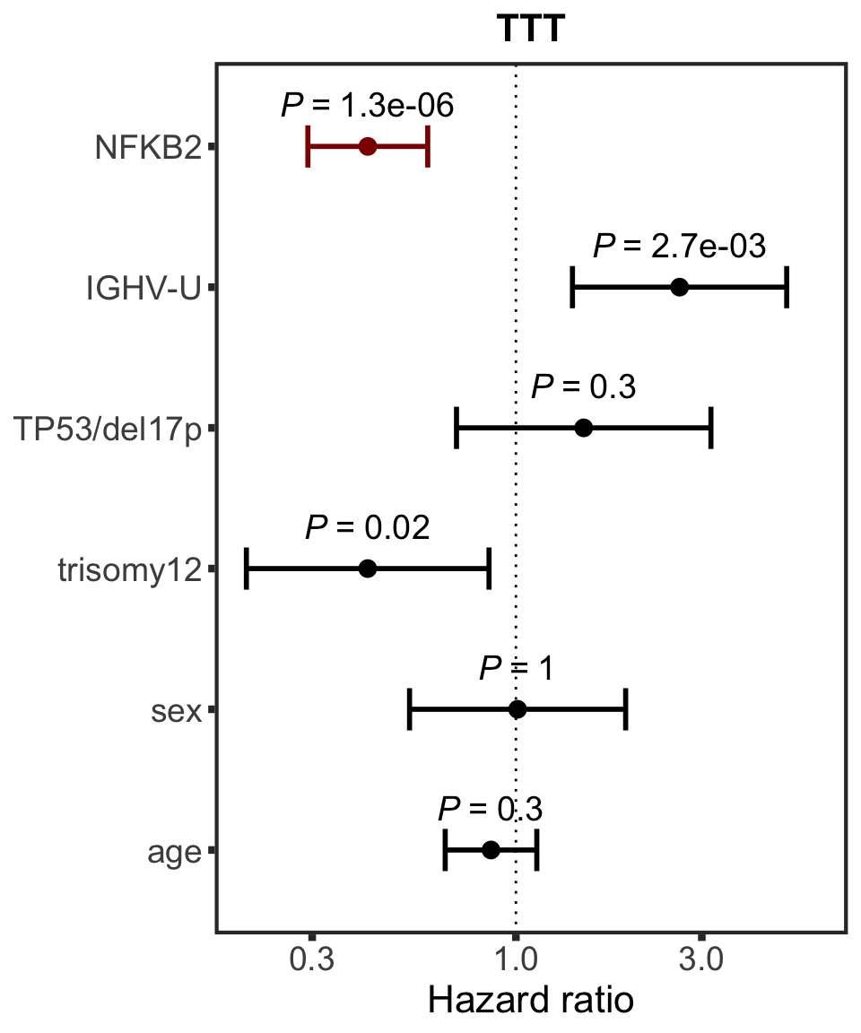
PURA
protName <- "PURA"
outcomeName <- "TTT"
survRes <- filter(cTab, outcome == outcomeName , name == protName)$fullModel[[1]]
hr.prmt5 <- plotHazard(survRes, protName, outcomeName)
hr.prmt5
PRMT5
protName <- "PRMT5"
outcomeName <- "TTT"
survRes <- filter(cTab, outcome == outcomeName , name == protName)$fullModel[[1]]
hr.prmt5 <- plotHazard(survRes, protName, "Time to treatment")
hr.prmt5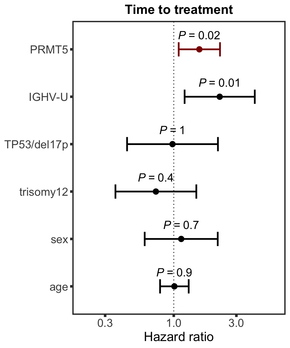
PYGB
protName <- "PYGB"
outcomeName <- "TTT"
survRes <- filter(cTab, outcome == outcomeName , name == protName)$fullModel[[1]]
hr.pygb <- plotHazard(survRes, protName, "Time to treatment")
hr.pygb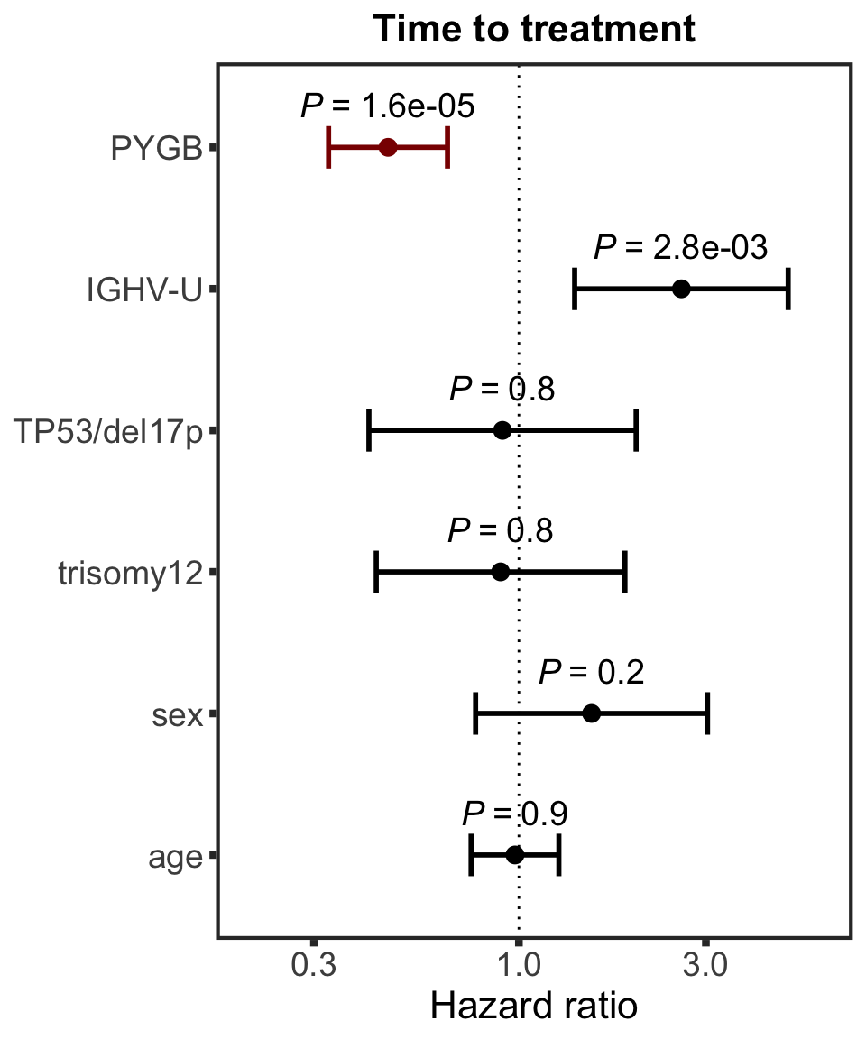
PES1
protName <- "PES1"
outcomeName <- "TTT"
survRes <- filter(cTab, outcome == outcomeName , name == protName)$fullModel[[1]]
hr.pes1 <- plotHazard(survRes, protName, "Time to treatment")
hr.pes1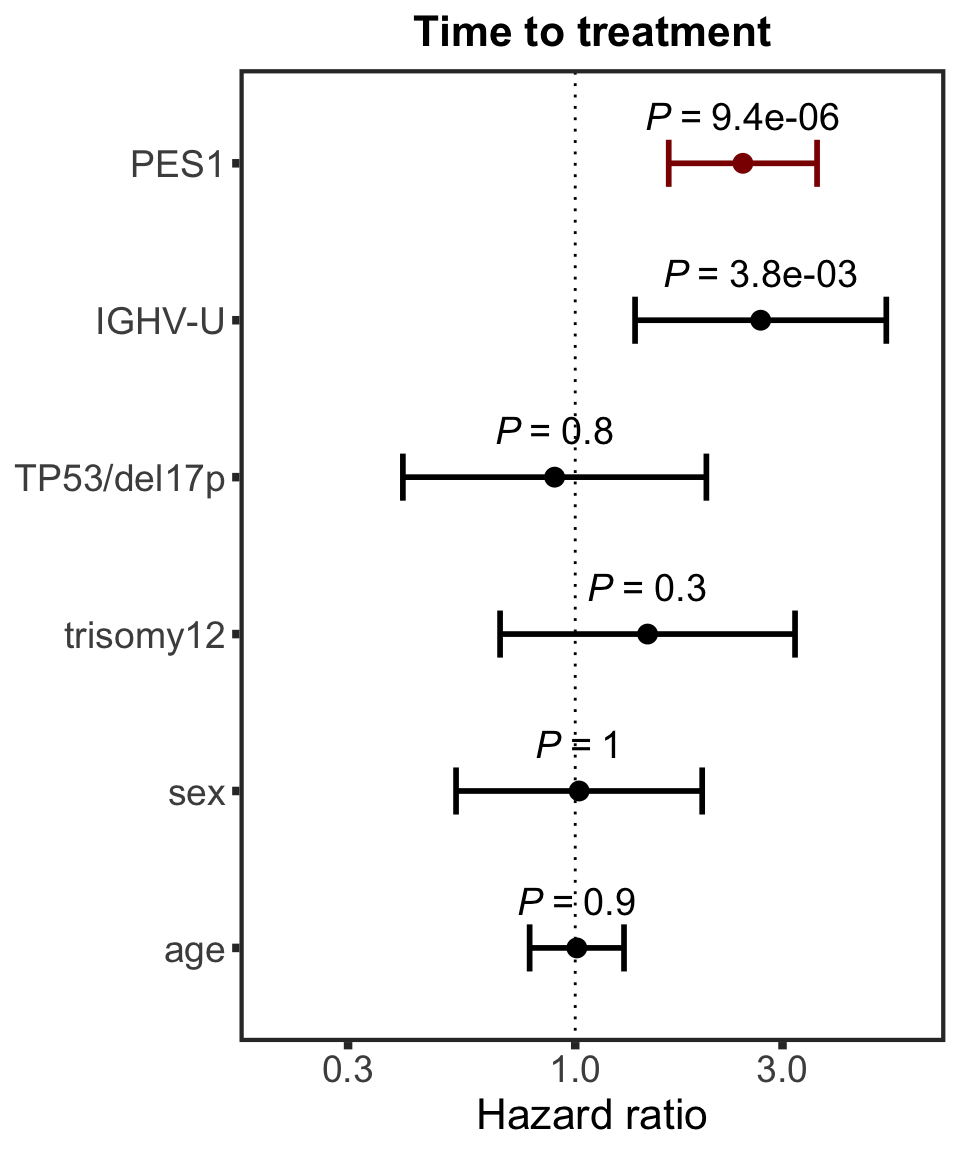
RRAS2
protName <- "RRAS2"
outcomeName <- "OS"
survRes <- filter(cTab, outcome == outcomeName , name == protName)$fullModel[[1]]
hr.rras <- plotHazard(survRes, protName, outcomeName)
hr.rras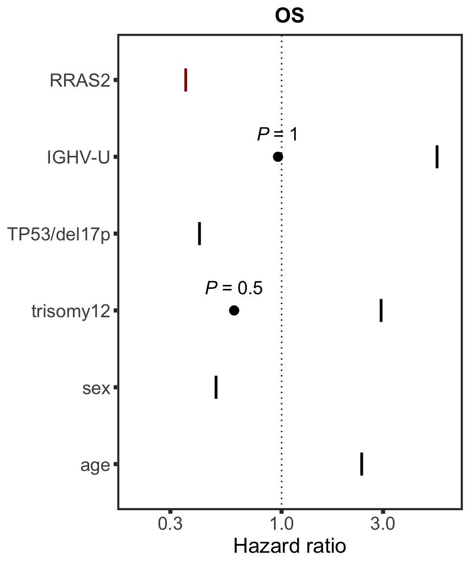
Clinical model without proteins (only including known risks in the multivariate model)
TTT
nullModelTTT <- runCox(survTab, riskTab, "TTT","treatedAfter")
pTTT<-plotHazard(nullModelTTT, "known risks", "TTT")
pTTT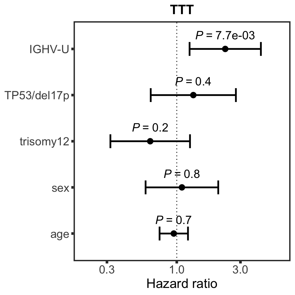
OS
nullModelOS <- runCox(survTab, riskTab, "OS","died")
pOS <- plotHazard(nullModelOS, "known risks", "OS", xLim = c(0.01,20))
pOS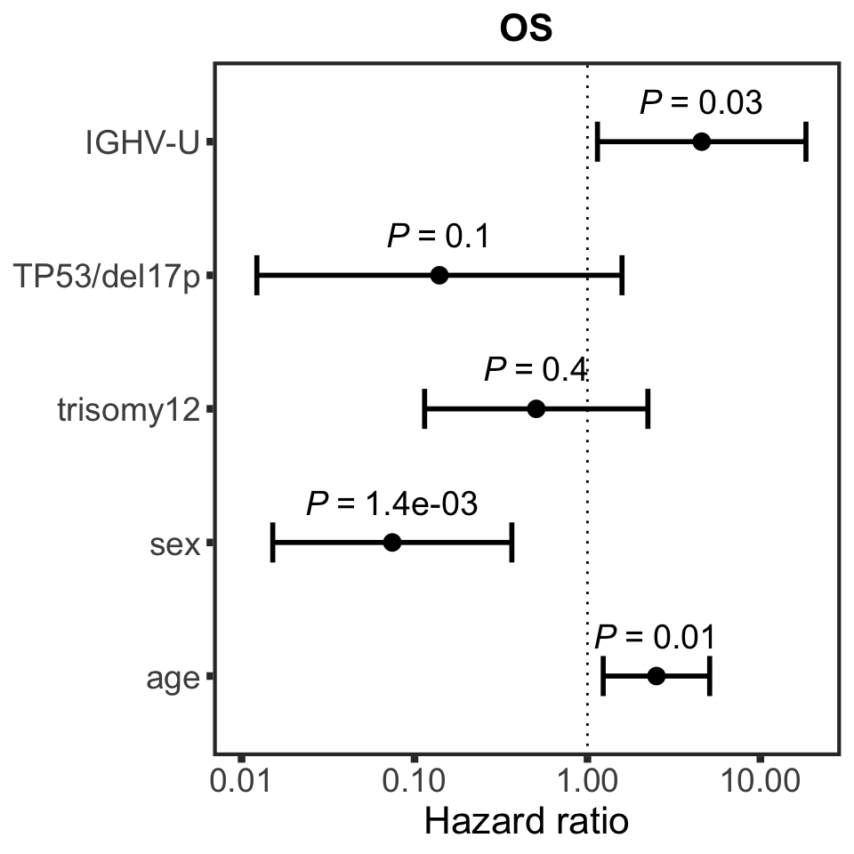
sessionInfo()R version 4.0.2 (2020-06-22)
Platform: x86_64-apple-darwin17.0 (64-bit)
Running under: macOS 10.16
Matrix products: default
BLAS: /Library/Frameworks/R.framework/Versions/4.0/Resources/lib/libRblas.dylib
LAPACK: /Library/Frameworks/R.framework/Versions/4.0/Resources/lib/libRlapack.dylib
locale:
[1] en_US.UTF-8/en_US.UTF-8/en_US.UTF-8/C/en_US.UTF-8/en_US.UTF-8
attached base packages:
[1] parallel stats4 stats graphics grDevices utils datasets
[8] methods base
other attached packages:
[1] ggbeeswarm_0.6.0 latex2exp_0.4.0
[3] forcats_0.5.1 stringr_1.4.0
[5] dplyr_1.0.5 purrr_0.3.4
[7] readr_1.4.0 tidyr_1.1.3
[9] tibble_3.1.0 tidyverse_1.3.0
[11] cowplot_1.1.1 SummarizedExperiment_1.18.2
[13] DelayedArray_0.14.1 matrixStats_0.58.0
[15] Biobase_2.48.0 GenomicRanges_1.40.0
[17] GenomeInfoDb_1.24.2 IRanges_2.22.2
[19] S4Vectors_0.26.1 BiocGenerics_0.34.0
[21] glmnet_4.1-1 Matrix_1.3-2
[23] ggraph_2.0.5 tidygraph_1.2.0
[25] igraph_1.2.6 maxstat_0.7-25
[27] survminer_0.4.9 ggpubr_0.4.0
[29] ggplot2_3.3.3 survival_3.2-7
[31] jyluMisc_0.1.5 pheatmap_1.0.12
[33] limma_3.44.3
loaded via a namespace (and not attached):
[1] utf8_1.1.4 shinydashboard_0.7.1 tidyselect_1.1.0
[4] htmlwidgets_1.5.3 grid_4.0.2 BiocParallel_1.22.0
[7] munsell_0.5.0 codetools_0.2-18 DT_0.17
[10] withr_2.4.1 colorspace_2.0-0 highr_0.8
[13] knitr_1.31 rstudioapi_0.13 ggsignif_0.6.1
[16] labeling_0.4.2 git2r_0.28.0 slam_0.1-48
[19] GenomeInfoDbData_1.2.3 KMsurv_0.1-5 polyclip_1.10-0
[22] farver_2.1.0 rprojroot_2.0.2 vctrs_0.3.6
[25] generics_0.1.0 TH.data_1.0-10 xfun_0.21
[28] sets_1.0-18 R6_2.5.0 graphlayouts_0.7.1
[31] bitops_1.0-6 fgsea_1.14.0 assertthat_0.2.1
[34] promises_1.2.0.1 scales_1.1.1 multcomp_1.4-16
[37] beeswarm_0.3.1 gtable_0.3.0 sandwich_3.0-0
[40] workflowr_1.6.2 rlang_0.4.10 splines_4.0.2
[43] rstatix_0.7.0 broom_0.7.5 yaml_2.2.1
[46] abind_1.4-5 modelr_0.1.8 crosstalk_1.1.1
[49] backports_1.2.1 httpuv_1.5.5 tools_4.0.2
[52] relations_0.6-9 ellipsis_0.3.1 gplots_3.1.1
[55] jquerylib_0.1.3 RColorBrewer_1.1-2 Rcpp_1.0.6
[58] visNetwork_2.0.9 zlibbioc_1.34.0 RCurl_1.98-1.2
[61] viridis_0.5.1 zoo_1.8-9 haven_2.3.1
[64] ggrepel_0.9.1 cluster_2.1.1 exactRankTests_0.8-31
[67] fs_1.5.0 magrittr_2.0.1 data.table_1.14.0
[70] openxlsx_4.2.3 reprex_1.0.0 mvtnorm_1.1-1
[73] hms_1.0.0 shinyjs_2.0.0 mime_0.10
[76] evaluate_0.14 xtable_1.8-4 rio_0.5.26
[79] readxl_1.3.1 gridExtra_2.3 shape_1.4.5
[82] compiler_4.0.2 KernSmooth_2.23-18 crayon_1.4.1
[85] htmltools_0.5.1.1 mgcv_1.8-34 later_1.1.0.1
[88] lubridate_1.7.10 DBI_1.1.1 tweenr_1.0.1
[91] dbplyr_2.1.0 MASS_7.3-53.1 car_3.0-10
[94] cli_2.3.1 marray_1.66.0 pkgconfig_2.0.3
[97] km.ci_0.5-2 foreign_0.8-81 piano_2.4.0
[100] xml2_1.3.2 foreach_1.5.1 vipor_0.4.5
[103] bslib_0.2.4 XVector_0.28.0 drc_3.0-1
[106] rvest_1.0.0 digest_0.6.27 rmarkdown_2.7
[109] cellranger_1.1.0 fastmatch_1.1-0 survMisc_0.5.5
[112] curl_4.3 shiny_1.6.0 gtools_3.8.2
[115] lifecycle_1.0.0 nlme_3.1-152 jsonlite_1.7.2
[118] carData_3.0-4 viridisLite_0.3.0 fansi_0.4.2
[121] pillar_1.5.1 lattice_0.20-41 fastmap_1.1.0
[124] httr_1.4.2 plotrix_3.8-1 glue_1.4.2
[127] zip_2.1.1 iterators_1.0.13 ggforce_0.3.3
[130] stringi_1.5.3 sass_0.3.1 caTools_1.18.1