Last updated: 2021-05-06

Checks: 5 2

Knit directory: CLLproteomics_publish_revision/analysis/

This reproducible R Markdown analysis was created with workflowr (version 1.6.2). The Checks tab describes the reproducibility checks that were applied when the results were created. The Past versions tab lists the development history.

R Markdown file: uncommitted changes

The R Markdown is untracked by Git. To know which version of the R Markdown file created these results, you’ll want to first commit it to the Git repo. If you’re still working on the analysis, you can ignore this warning. When you’re finished, you can run wflow_publish to commit the R Markdown file and build the HTML.

Environment: empty

Great job! The global environment was empty. Objects defined in the global environment can affect the analysis in your R Markdown file in unknown ways. For reproduciblity it’s best to always run the code in an empty environment.

Seed: set.seed(20200227)

The command set.seed(20200227) was run prior to running the code in the R Markdown file. Setting a seed ensures that any results that rely on randomness, e.g. subsampling or permutations, are reproducible.

Session information: recorded

Great job! Recording the operating system, R version, and package versions is critical for reproducibility.

Cache: detected

The following chunks had caches available:

unnamed-chunk-12
unnamed-chunk-19
unnamed-chunk-26
unnamed-chunk-4
unnamed-chunk-5

To ensure reproducibility of the results, delete the cache directory manuscript_S9_STAT2_cache and re-run the analysis. To have workflowr automatically delete the cache directory prior to building the file, set delete_cache = TRUE when running wflow_build() or wflow_publish().

File paths: relative

Great job! Using relative paths to the files within your workflowr project makes it easier to run your code on other machines.

Repository version: 3fb50c5

Great! You are using Git for version control. Tracking code development and connecting the code version to the results is critical for reproducibility.

The results in this page were generated with repository version 3fb50c5. See the Past versions tab to see a history of the changes made to the R Markdown and HTML files.

Note that you need to be careful to ensure that all relevant files for the analysis have been committed to Git prior to generating the results (you can use wflow_publish or wflow_git_commit). workflowr only checks the R Markdown file, but you know if there are other scripts or data files that it depends on. Below is the status of the Git repository when the results were generated:


Ignored files:
    Ignored:    .DS_Store
    Ignored:    .Rhistory
    Ignored:    .Rproj.user/
    Ignored:    analysis/.DS_Store
    Ignored:    analysis/.Rhistory
    Ignored:    analysis/manuscript_S1_Overview_cache/
    Ignored:    analysis/manuscript_S2_genomicAssociation_cache/
    Ignored:    analysis/manuscript_S3_trisomy12_cache/
    Ignored:    analysis/manuscript_S4_IGHV_cache/
    Ignored:    analysis/manuscript_S5_trisomy19_cache/
    Ignored:    analysis/manuscript_S6_del11q_cache/
    Ignored:    analysis/manuscript_S8_drugResponse_Outcomes_cache/
    Ignored:    analysis/manuscript_S9_STAT2_cache/
    Ignored:    code/.DS_Store
    Ignored:    code/.Rhistory
    Ignored:    data/.DS_Store
    Ignored:    output/.DS_Store

Untracked files:
    Untracked:  analysis/.trisomy12_norm.pdf
    Untracked:  analysis/IGHV_box.pdf
    Untracked:  analysis/IGHV_enrich.pdf
    Untracked:  analysis/IGHV_volcano.pdf
    Untracked:  analysis/bufferComplexViolin.pdf
    Untracked:  analysis/buffer_Tri12vsTri19.pdf
    Untracked:  analysis/cohortComposition_all.pdf
    Untracked:  analysis/drugBar.pdf
    Untracked:  analysis/dubelisib_tri12.pdf
    Untracked:  analysis/heatmap_tri12_circle.pdf
    Untracked:  analysis/manuscript_S1_Overview.Rmd
    Untracked:  analysis/manuscript_S2_genomicAssociation.Rmd
    Untracked:  analysis/manuscript_S3_trisomy12.Rmd
    Untracked:  analysis/manuscript_S4_IGHV.Rmd
    Untracked:  analysis/manuscript_S5_trisomy19.Rmd
    Untracked:  analysis/manuscript_S6_del11q.Rmd
    Untracked:  analysis/manuscript_S7_SF3B1.Rmd
    Untracked:  analysis/manuscript_S8_drugResponse_Outcomes.Rmd
    Untracked:  analysis/manuscript_S9_STAT2.Rmd
    Untracked:  analysis/plot_PC1_PC2.pdf
    Untracked:  analysis/protDrugTP53.pdf
    Untracked:  analysis/timsTOF_validate.Rmd
    Untracked:  analysis/tri12_transEnrich.pdf
    Untracked:  analysis/tri19_dosage_effect.pdf
    Untracked:  analysis/tri19_sum_buffer_number.pdf
    Untracked:  analysis/trisomy12_chr_summary.pdf
    Untracked:  code/utils.R
    Untracked:  data/Annotation file March 2021.xlsx
    Untracked:  data/CAS9results.xlsx
    Untracked:  data/CNV_onChrom.RData
    Untracked:  data/ComplexParticipantsPubMedIdentifiers_human.txt
    Untracked:  data/Fig1A.png
    Untracked:  data/IGLV321_SupplementalTables_R2.xlsx
    Untracked:  data/MOFAout.RData
    Untracked:  data/MOFAout_atLeast3.RData
    Untracked:  data/STATexprPCR.xlsx
    Untracked:  data/Western_blot_results_20210309_short.csv
    Untracked:  data/Western_blot_results_separate_blots.xlsx
    Untracked:  data/allComplexes.txt
    Untracked:  data/ddsrna_enc.RData
    Untracked:  data/exprCNV_enc.RData
    Untracked:  data/geneAnno.RData
    Untracked:  data/gmts/
    Untracked:  data/ic50.RData
    Untracked:  data/mofaIn.RData
    Untracked:  data/mofaIn_atLeast3.RData
    Untracked:  data/patMeta_enc.RData
    Untracked:  data/pepCLL_lumos_enc.RData
    Untracked:  data/protMOFA.RData
    Untracked:  data/proteins_in_complexes
    Untracked:  data/proteomic_LUMOS_2pep_enc.RData
    Untracked:  data/proteomic_explore_enc.RData
    Untracked:  data/proteomic_independent_all_enc.RData
    Untracked:  data/proteomic_independent_enc.RData
    Untracked:  data/proteomic_timsTOF_enc.RData
    Untracked:  data/screenData_enc.RData
    Untracked:  data/setToPathway.txt
    Untracked:  data/survival_enc.RData
    Untracked:  output/MSH6_splicing.svg
    Untracked:  output/SUGP1_splicing.svg
    Untracked:  output/deResList.RData
    Untracked:  output/deResListBatch2.RData
    Untracked:  output/deResListRNA.RData
    Untracked:  output/deResListRNA_allGene.RData
    Untracked:  output/deResList_WBC.RData
    Untracked:  output/deResList_batch1.RData
    Untracked:  output/deResList_batch3.RData
    Untracked:  output/deResList_independent.RData
    Untracked:  output/deResList_timsTOF.RData
    Untracked:  output/dxdCLL.RData
    Untracked:  output/dxdCLL2.RData
    Untracked:  output/exprCNV.RData
    Untracked:  output/geneAnno.RData
    Untracked:  output/int_pairs.csv
    Untracked:  output/lassoResults_CPS.RData
    Untracked:  output/resOutcome_batch1.RData
    Untracked:  output/resOutcome_batch13.RData
    Untracked:  output/resOutcome_batch2.RData
    Untracked:  output/resOutcome_batch3.RData

Unstaged changes:
    Modified:   analysis/_site.yml
    Deleted:    analysis/analysisSF3B1.Rmd
    Deleted:    analysis/comparePlatforms.Rmd
    Deleted:    analysis/compareProteomicsRNAseq.Rmd
    Deleted:    analysis/correlateCLLPD.Rmd
    Deleted:    analysis/correlateGenomic.Rmd
    Deleted:    analysis/correlateGenomic_removePC.Rmd
    Deleted:    analysis/correlateMIR.Rmd
    Deleted:    analysis/correlateMethylationCluster.Rmd
    Modified:   analysis/index.Rmd
    Deleted:    analysis/predictOutcome.Rmd
    Deleted:    analysis/processProteomics_LUMOS.Rmd
    Deleted:    analysis/processProteomics_timsTOF.Rmd
    Deleted:    analysis/qualityControl_LUMOS.Rmd
    Deleted:    analysis/qualityControl_timsTOF.Rmd

Note that any generated files, e.g. HTML, png, CSS, etc., are not included in this status report because it is ok for generated content to have uncommitted changes.

There are no past versions. Publish this analysis with wflow_publish() to start tracking its development.

Load packages and datasets

library(cowplot)
library(piano)
library(pheatmap)
library(ComplexHeatmap)
library(jyluMisc)
library(limma)
library(gtable)
library(ggbeeswarm)
library(glmnet)
library(SummarizedExperiment)
library(tidyverse)

#load datasets
load("../data/patMeta_enc.RData")
load("../data/ddsrna_enc.RData")
load("../data/proteomic_explore_enc.RData")
load("../output/deResList.RData") #precalculated differential expression
load("../data/screenData_enc.RData")

# source 
source("../code/utils.R")

Feature selection with LASSO on multi-omic data to explain STAT2 protein expression

Preprocessing multi-omic data

Proteomics data

expVar <- "STAT2"

protMat <- assays(protCLL)[["QRILC_combat"]]
rownames(protMat) <- rowData(protCLL)$hgnc_symbol

yVec <- protMat[expVar,]
protMat <- protMat[rownames(protMat) != expVar,]

## Pre-filter for significant associations
designMat <- model.matrix(~yVec)
fit <- lmFit(protMat, design = designMat)
fit2 <- eBayes(fit)
resTab <- topTable(fit2, number = Inf)
keepProt <- filter(resTab, adj.P.Val < 0.05)$ID
protMat <- t(protMat[keepProt, ])
dim(protMat)

[1]  91 474

responseList <- list()
responseList[["STAT2"]] <- yVec

colnames(protMat) <- paste0(colnames(protMat),"_protein")

RNAseq

#subset
ddsSub <- dds[,dds$PatID %in% colnames(protCLL)]

#only keep protein coding genes with symbol
ddsSub <- ddsSub[rowData(ddsSub)$biotype %in% "protein_coding" & rowData(ddsSub)$symbol %in% rowData(protCLL)$hgnc_symbol,]

#remove lowly expressed genes
ddsSub <- ddsSub[rowSums(counts(ddsSub, normalized = TRUE)) > 100,]

#voom transformation
ddsSub.vst <- varianceStabilizingTransformation(ddsSub)
exprMat <- assay(ddsSub.vst)

rnaMat <- exprMat
rownames(rnaMat) <- rowData(ddsSub.vst)$symbol
# Prefiltering
overSampe <- intersect(names(yVec), colnames(rnaMat))
designMat <- model.matrix(~ yVec[overSampe])
fit <- lmFit(rnaMat[,overSampe], design = designMat)
fit2 <- eBayes(fit)
resTab <- topTable(fit2, number = Inf) %>% data.frame() %>% rownames_to_column("ID")
keepRna <- filter(resTab, adj.P.Val < 0.05)$ID
rnaMat <- t(rnaMat[keepRna, ])
dim(rnaMat)

[1]  82 156

colnames(rnaMat) <- paste0(colnames(rnaMat),"_rna")

Genomic data

ighvMap <- c(M = 1, U=0)
methMap <- c(LP= 0, IP=0.5, HP=1 )

#genetics
genData <- filter(patMeta, Patient.ID %in% colnames(protCLL)) %>%
  dplyr::rename(IGHV = IGHV.status) %>%
  mutate_at(vars(-Patient.ID), as.character) %>%
  mutate(IGHV = ighvMap[IGHV]) %>%
  mutate_at(vars(-Patient.ID), as.numeric) %>%
  data.frame() %>% column_to_rownames("Patient.ID")

#remove gene with higher than 40% missing values
genData <- genData[,colSums(is.na(genData))/nrow(genData) <= 0.4]

#remove genes with less than 5 mutated cases
genData <- genData[,colSums(genData, na.rm = TRUE) >= 5]  

#fill the missing value with majority
genData <- apply(genData, 2, function(x) {
  xVec <- x
  avgVal <- mean(x,na.rm= TRUE)
  if (avgVal >= 0.5) {
    xVec[is.na(xVec)] <- 1
  } else xVec[is.na(xVec)] <- 0
  xVec
})

Drug responses

#choose the first sample
viabMat <- arrange(screenData, screenDate) %>%
  filter(diagnosis == "CLL", patientID %in% colnames(protCLL)) %>%
  distinct(patientID, Drug, concIndex, .keep_all = TRUE) %>%
  filter(! Drug %in% c("DMSO","PBS")) %>%
  mutate(id = paste0(Drug,"_",concIndex)) %>%
  select(patientID, id, normVal.adj.sigm) %>%
  spread(key = patientID, value = normVal.adj.sigm) %>%
  data.frame() %>% column_to_rownames("id") %>% 
  as.matrix() %>% t()

Feature selection with LASSO (L1) penalty

#Functions for running glm
runGlm <- function(X, y, method = "ridge", repeats=20, folds = 3, lambda = "lambda.1se") {
  modelList <- list()
  lambdaList <- c()
  varExplain <- c()
  coefMat <- matrix(NA, ncol(X), repeats)
  rownames(coefMat) <- colnames(X)

  if (method == "lasso"){
    alpha = 1
  } else if (method == "ridge") {
    alpha = 0
  }
  
  for (i in seq(repeats)) {
    if (ncol(X) > 2) {
      res <- cv.glmnet(X,y, type.measure = "mse", family="gaussian", 
                       nfolds = folds, alpha = alpha, standardize = FALSE)
      lambdaList <- c(lambdaList, res[[lambda]])
      modelList[[i]] <- res
      
      coefModel <- coef(res, s = lambda)[-1] #remove intercept row
      coefMat[,i] <- coefModel
      
      #calculate variance explained
      y.pred <- predict(res, s = lambda, newx = X)
      varExp <- cor(as.vector(y),as.vector(y.pred))^2
      varExplain[i] <- ifelse(is.na(varExp), 0, varExp) 
      
    } else {
      fitlm<-lm(y~., data.frame(X))
      varExp <- summary(fitlm)$r.squared
      varExplain <- c(varExplain, varExp)
      
    }

  }
  list(modelList = modelList, lambdaList = lambdaList, varExplain = varExplain, coefMat = coefMat)
}

#function for scaling predictors
dataScale <- function(x, censor = NULL, robust = FALSE) {
        #function to scale different variables
        if (length(unique(na.omit(x))) <=3){
          #a binary variable, change to -0.5 and 0.5 for 1 and 2
          x - 0.5
        } else {
          if (robust) {
          #continuous variable, centered by median and divied by 2*mad
          mScore <- (x-median(x,na.rm=TRUE))/mad(x,na.rm=TRUE)
            if (!is.null(censor)) {
              mScore[mScore > censor] <- censor
              mScore[mScore < -censor] <- -censor
            }
          mScore/2
          } else {
            mScore <- (x-mean(x,na.rm=TRUE))/(sd(x,na.rm=TRUE))
              if (!is.null(censor)) {
                mScore[mScore > censor] <- censor
                mScore[mScore < -censor] <- -censor
              }
          mScore/2
          }
        }
      }

#function to generate response vector and explainatory variable for each seahorse measurement
generateData <- function(responseList, inclSet,  onlyCombine = FALSE, censor = NULL, robust = FALSE) {
    
    allResponse <- list()
    allExplain <- list()

    for (measure in names(responseList)) {
      y <- responseList[[measure]]
      y <- y[!is.na(y)]
      
      #get overlapped samples for each dataset 
      overSample <- names(y)
      
      for (eachSet in inclSet) {
        overSample <- intersect(overSample,rownames(eachSet))
      }
      
      y <- dataScale(y[overSample], censor = censor, robust = robust)
      
      expTab <- list()
      
      if ("Gene" %in% names(inclSet)) {
        geneTab <- inclSet$Gene[overSample,]
        #at least 3 mutated sample
        geneTab <- geneTab[, colSums(geneTab) >= 3]
        vecName <- sprintf("genetic(%s)", ncol(geneTab))
        expTab[[vecName]] <- apply(geneTab,2,dataScale)
      }
      
      
      if ("RNA" %in% names(inclSet)){
        rnaMat <- inclSet$RNA[overSample, ]
        colnames(rnaMat) <- paste0("con.",colnames(rnaMat), sep = "")
        vecName <- sprintf("RNA(%s)", ncol(rnaMat))
        expTab[[vecName]] <- apply(rnaMat,2,dataScale, censor = censor, robust = robust)
        
      }
      
      if ("Protein" %in% names(inclSet)){
        protMat <- inclSet$Protein[overSample, ]
        colnames(protMat) <- paste0("con.",colnames(protMat), sep = "")
        vecName <- sprintf("Protein(%s)", ncol(protMat))
        expTab[[vecName]] <- apply(protMat,2,dataScale, censor = censor, robust = robust)
        
      }
        
      if ("Drug" %in% names(inclSet)){
        drugMat <- inclSet$Drug[overSample, ]
        colnames(drugMat) <- paste0("con.",colnames(drugMat), sep = "")
        vecName <- sprintf("Drug(%s)", ncol(drugMat))
        expTab[[vecName]] <- apply(drugMat,2,dataScale, censor = censor, robust = robust)
        
      }
      
      comboTab <- c()
      for (eachSet in names(expTab)){
        comboTab <- cbind(comboTab, expTab[[eachSet]])
      }
      vecName <- sprintf("all(%s)", ncol(comboTab))
      expTab[[vecName]] <- comboTab
      
      allResponse[[measure]] <- y
      allExplain[[measure]] <- expTab
    }
  if (onlyCombine) {
    #only return combined results, for feature selection
    allExplain <- lapply(allExplain, function(x) x[length(x)])
  }
    
  return(list(allResponse=allResponse, allExplain=allExplain))

}

Clean and integrate multi-omics data

inclSet<-list(Gene=genData, RNA = rnaMat, Protein = protMat)
cleanData <- generateData(responseList, inclSet, censor = 5)

#Function for multi-variate regression

runGlm <- function(X, y, method = "ridge", repeats=20, folds = 3) {
  modelList <- list()
  lambdaList <- c()
  varExplain <- c()
  coefMat <- matrix(NA, ncol(X), repeats)
  rownames(coefMat) <- colnames(X)

  if (method == "lasso"){
    alpha = 1
  } else if (method == "ridge") {
    alpha = 0
  }
  
  for (i in seq(repeats)) {
    if (ncol(X) > 2) {
      res <- cv.glmnet(X,y, type.measure = "mse", family="gaussian", 
                       nfolds = folds, alpha = alpha, standardize = FALSE)
      lambdaList <- c(lambdaList, res$lambda.min)
      modelList[[i]] <- res
      
      coefModel <- coef(res, s = "lambda.min")[-1] #remove intercept row
      coefMat[,i] <- coefModel
      
      #calculate variance explained
      y.pred <- predict(res, s = "lambda.min", newx = X)
      
      varExp <- 1-min(res$cvm)/res$cvm[1]
      #varExp <- cor(as.vector(y),as.vector(y.pred))^2
      varExplain[i] <- ifelse(is.na(varExp), 0, varExp) 
      
    } else {
      fitlm<-lm(y~., data.frame(X))
      varExp <- summary(fitlm)$r.squared
      varExplain <- c(varExplain, varExp)
      
    }

  }
  list(modelList = modelList, lambdaList = lambdaList, varExplain = varExplain, coefMat = coefMat)
}

set.seed(2021)
lassoResults <- list()
for (eachMeasure in names(cleanData$allResponse)) {
  dataResult <- list()
  for (eachDataset in names(cleanData$allExplain[[eachMeasure]])) {
    y <- cleanData$allResponse[[eachMeasure]]
    X <- cleanData$allExplain[[eachMeasure]][[eachDataset]]
  
   
    glmRes <- runGlm(X, y, method = "lasso", repeats = 50, folds = 3)
    dataResult[[eachDataset]] <- glmRes 
  }
  lassoResults[[eachMeasure]] <- dataResult
  
}

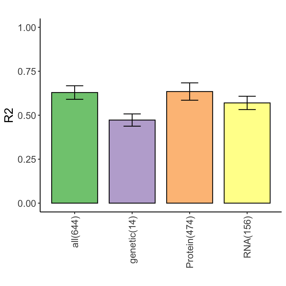
Variance explained for STAT2 expression by multi-omics datasets

Heatmap of selected features

library(gtable)
lassoPlot <- function(lassoOut, cleanData, freqCut = 1, coefCut = 0.01, setNumber = "last", legend = TRUE, labSuffix = " protein expression", scaleFac =1) {
  plotList <- list()
  if (setNumber == "last") {
    setNumber <- length(lassoOut[[1]])
  } else {
    setNumber <- setNumber
  }
  for (seaName in names(lassoOut)) {
    #for the barplot on the left of the heatmap
    barValue <- rowMeans(lassoOut[[seaName]][[setNumber]]$coefMat)
    freqValue <- rowMeans(abs(sign(lassoOut[[seaName]][[setNumber]]$coefMat)))
    barValue <- barValue[abs(barValue) >= coefCut & freqValue >= freqCut] # a certain threshold
    barValue <- barValue[order(barValue)]
    if(length(barValue) == 0) {
      plotList[[seaName]] <- NA
      next
    }

    #for the heatmap and scatter plot below the heatmap
    allData <- cleanData$allExplain[[seaName]][[setNumber]]
    seaValue <- cleanData$allResponse[[seaName]]*2 #back to Z-score
    
    tabValue <- allData[, names(barValue),drop=FALSE]
    ord <- order(seaValue)
    seaValue <- seaValue[ord]
    tabValue <- tabValue[ord, ,drop=FALSE]
    sampleIDs <- rownames(tabValue)
    tabValue <- as.tibble(tabValue)
    
    #change scaled binary back to catagorical
    for (eachCol in colnames(tabValue)) {
      if (strsplit(eachCol, split = "[.]")[[1]][1] != "con") {
        tabValue[[eachCol]] <- as.integer(as.factor(tabValue[[eachCol]]))
      }
      else {
        tabValue[[eachCol]] <- tabValue[[eachCol]]*2 #back to Z-score
      }
    }
    
    tabValue$Sample <- sampleIDs
    #Mark different rows for different scaling in heatmap
    matValue <- gather(tabValue, key = "Var",value = "Value", -Sample)
    matValue$Type <- "mut"
    
    #For continuious value
    matValue$Type[grep("con.",matValue$Var)] <- "con"
    
    #for methylation_cluster
    matValue$Type[grep("ConsCluster",matValue$Var)] <- "meth"
    
    #change the scale of the value, let them do not overlap with each other
    matValue[matValue$Type == "mut",]$Value = matValue[matValue$Type == "mut",]$Value + 10
    matValue[matValue$Type == "meth",]$Value = matValue[matValue$Type == "meth",]$Value + 20
    
    
    #color scale for viability
    idx <- matValue$Type == "con"
    
    myCol <- colorRampPalette(c(colList[2],'white',colList[1]), 
                   space = "Lab")
    if (sum(idx) != 0) {
      matValue[idx,]$Value = round(matValue[idx,]$Value,digits = 2)
      minViab <- min(matValue[idx,]$Value)
      maxViab <- max(matValue[idx,]$Value)
      limViab <- max(c(abs(minViab), abs(maxViab)))
      scaleSeq1 <- round(seq(-limViab, limViab,0.01), digits=2)
      color4viab <- setNames(myCol(length(scaleSeq1+1)), nm=scaleSeq1)
    } else {
      scaleSeq1 <- round(seq(0,1,0.01), digits=2)
      color4viab <- setNames(myCol(length(scaleSeq1+1)), nm=scaleSeq1)
    }
    

    
    #change continues measurement to discrete measurement
    matValue$Value <- factor(matValue$Value,levels = sort(unique(matValue$Value)))
    
    #change order of heatmap
    names(barValue) <-  gsub("con.", "", names(barValue))
    matValue$Var <- gsub("con.","",matValue$Var)
    matValue$Var <- factor(matValue$Var, levels = names(barValue))
    matValue$Sample <- factor(matValue$Sample, levels = names(seaValue))
    #plot the heatmap
    p1 <- ggplot(matValue, aes(x=Sample, y=Var)) + geom_tile(aes(fill=Value), color = "gray") + 
      theme_bw() + scale_y_discrete(expand=c(0,0),position = "right") + 
      theme(axis.text.y=element_text(hjust=0, size=10*scaleFac), axis.text.x=element_blank(), 
            axis.title = element_blank(),
            axis.ticks=element_blank(), panel.border=element_rect(colour="gainsboro"),  
            plot.title=element_blank(), panel.background=element_blank(), 
            panel.grid.major=element_blank(), panel.grid.minor=element_blank(),
            plot.margin = margin(0,0,0,0)) +  
      scale_fill_manual(name="Mutated",  values=c(color4viab, `11`="gray96", `12`='black', `21`='lightgreen', 
                                                       `22`='green',`23` = 'green4'),guide=FALSE) #+ ggtitle(seaName)
    
    #Plot the bar plot on the left of the heatmap
    barDF = data.frame(barValue, nm=factor(names(barValue),levels=names(barValue)))
    
    p2 <- ggplot(data=barDF, aes(x=nm, y=barValue)) + 
      geom_bar(stat="identity", fill=colList[6], colour="black", position = "identity", width=.66, size=0.2) + 
      theme_bw() + geom_hline(yintercept=0, size=0.3) + scale_x_discrete(expand=c(0,0.5)) + 
      scale_y_continuous(expand=c(0,0)) + coord_flip() + 
      theme(panel.grid.major=element_blank(), panel.background=element_blank(), axis.ticks.y = element_blank(),
            panel.grid.minor = element_blank(), 
            axis.text.x =element_text(size=8*scaleFac), 
            axis.text.y = element_blank(),
            axis.title = element_blank(),
            panel.border=element_blank(),plot.margin = margin(0,0,0,0))  + geom_vline(xintercept=c(0.5), color="black", size=0.6)
    
    #Plot the scatter plot under the heatmap
    
    # scatterplot below
    scatterDF = data.frame(X=factor(names(seaValue), levels=names(seaValue)), Y=seaValue)
    
    p3 <- ggplot(scatterDF, aes(x=X, y=Y)) + geom_point(shape=21, fill="dimgrey", colour="black", size=1.2) + 
      xlab(paste0(seaName, labSuffix)) + ylab("Z-score") +
      theme_bw() + 
      theme(panel.grid.minor=element_blank(), panel.grid.major.x=element_blank(), 
            axis.title=element_text(size=10*scaleFac), 
            axis.text.x=element_blank(), axis.ticks.x=element_blank(), 
            axis.text.y=element_text(size=8*scaleFac), 
            panel.border=element_rect(colour="dimgrey", size=0.1), 
            panel.background=element_rect(fill="gray96"),plot.margin = margin(0,0,0,0))
    
     
    dummyGrob <- ggplot() + theme_void()
    
    #Scale bar for continuous variable
    if (legend) {
       Vgg = ggplot(data=data.frame(x=1, y=as.numeric(names(color4viab))), aes(x=x, y=y, color=y)) + geom_point() + 
      scale_color_gradientn(name="Z-score", colours =color4viab) + 
      theme(legend.title=element_text(size=12*scaleFac), legend.text=element_text(size=10*scaleFac))
    barLegend <- plot_grid(gtable_filter(ggplotGrob(Vgg), "guide-box"))
    #Assemble all the plots togehter
    } else {
     barLegend <- dummyGrob  
    }
   
    
   
    gt <- egg::ggarrange(p2,p1,barLegend,dummyGrob, p3, dummyGrob, ncol=3, nrow=2, 
                         widths = c(0.6,2,0.3), padding = unit(0,"line"), clip = "off",
                         heights = c(length(unique(matValue$Var))/2,2),draw = FALSE)
    plotList[[seaName]] <- gt
  }
  return(plotList)
}

Genetics only

heatMaps <- lassoPlot(lassoResults, cleanData, freqCut = 1,setNumber = 1, legend = FALSE, scaleFac = 1)

heatMaps <- heatMaps[!is.na(heatMaps)]
geneLasso <- plot_grid(plotlist=heatMaps, ncol=1)
geneLasso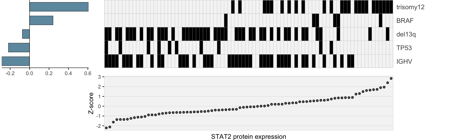

Combined

heatMaps <- lassoPlot(lassoResults, cleanData, freqCut = 1,setNumber = 4, legend = TRUE,  scaleFac = 1)

heatMaps <- heatMaps[!is.na(heatMaps)]
comLasso <- plot_grid(plotlist=heatMaps, ncol=1)
comLasso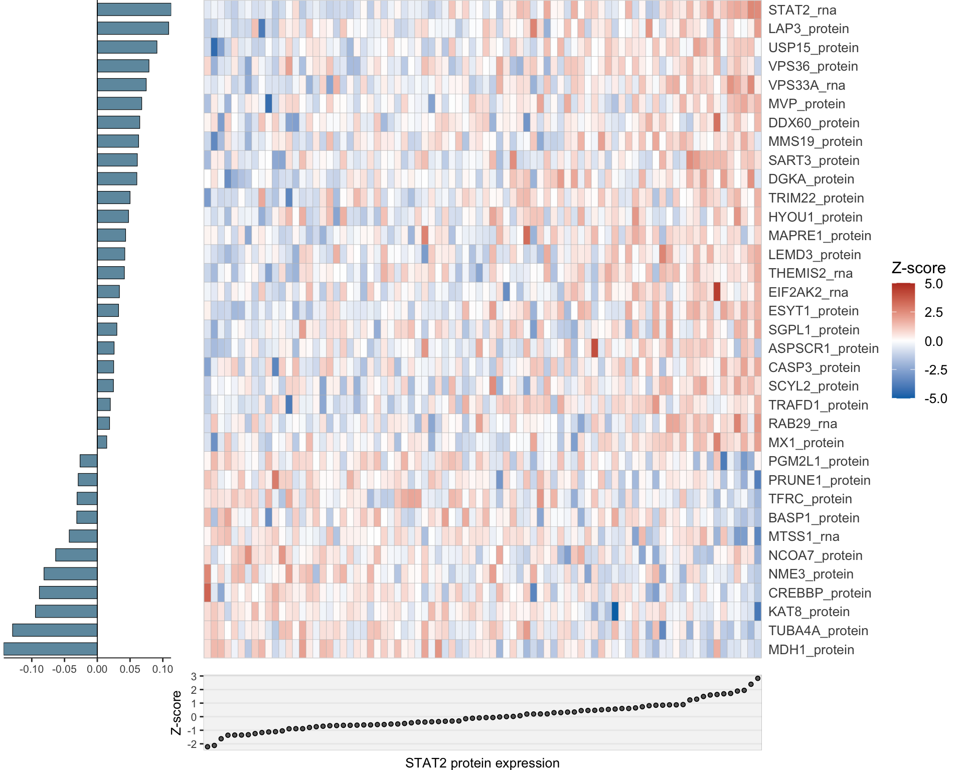

LASSO model with only protein and RNA combined

Clean and integrate multi-omics data

inclSet<-list(RNA = rnaMat, Protein = protMat)
cleanData <- generateData(responseList, inclSet, censor = 5)

set.seed(2020)
lassoResults <- list()
for (eachMeasure in names(cleanData$allResponse)) {
  dataResult <- list()
  for (eachDataset in names(cleanData$allExplain[[eachMeasure]])) {
    y <- cleanData$allResponse[[eachMeasure]]
    X <- cleanData$allExplain[[eachMeasure]][[eachDataset]]
  
   
    glmRes <- runGlm(X, y, method = "lasso", repeats = 50, folds = 3)
    dataResult[[eachDataset]] <- glmRes 
  }
  lassoResults[[eachMeasure]] <- dataResult
  
}

heatMaps <- lassoPlot(lassoResults, cleanData, freqCut = 1,setNumber = 3, legend = TRUE,  scaleFac = 1)

heatMaps <- heatMaps[!is.na(heatMaps)]
comLasso <- plot_grid(plotlist=heatMaps, ncol=1)
comLasso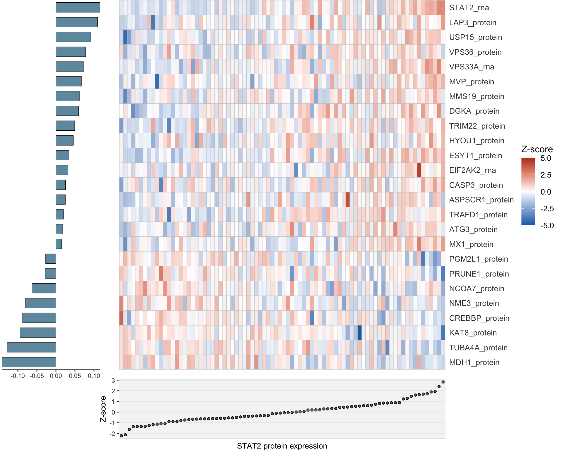

IGHV mutational status and trisomy12 status jointly determine STAT2 protein expression

ANOVA test on IGHV/trisomy12 status to STAT2 protein expression

plotTab <- tibble(patID = colnames(protCLL),
                  STAT2 = assays(protCLL)[["count_combat"]][rowData(protCLL)$hgnc_symbol == "STAT2",],
                  trisomy12 = protCLL$trisomy12,
                  IGHV=protCLL$IGHV.status) %>%
  filter(!is.na(IGHV), !is.na(trisomy12)) %>%
  mutate(trisomy12 = ifelse(trisomy12 == 0, "non-tri12","tri12")) %>%
  mutate(group = paste0(IGHV, "_", trisomy12))
stat2BoxProt <- ggplot(plotTab, aes(group, y=STAT2, fill = group)) + geom_boxplot() + geom_point() + theme_full +
  scale_fill_manual(values = colList) + theme(legend.position = "none") +
  xlab("") + ggtitle("STAT2 protein expression") +ylab("Normalized expression")

summary(lm(STAT2 ~ IGHV * trisomy12, plotTab))


Call:
lm(formula = STAT2 ~ IGHV * trisomy12, data = plotTab)

Residuals:
    Min      1Q  Median      3Q     Max 
-0.9044 -0.2317 -0.0275  0.2222  0.8272 

Coefficients:
                     Estimate Std. Error t value Pr(>|t|)    
(Intercept)          15.79174    0.06256 252.427  < 2e-16 ***
IGHVU                 0.18836    0.09073   2.076 0.040846 *  
trisomy12tri12        0.43065    0.11074   3.889 0.000196 ***
IGHVU:trisomy12tri12  0.41597    0.15789   2.634 0.009974 ** 
---
Signif. codes:  0 '***' 0.001 '**' 0.01 '*' 0.05 '.' 0.1 ' ' 1

Residual standard error: 0.3539 on 87 degrees of freedom
Multiple R-squared:  0.5157,    Adjusted R-squared:  0.499 
F-statistic: 30.87 on 3 and 87 DF,  p-value: 1.097e-13

STAT2 protein expression is strongly affected by IGHV and trisomy12 status, U-CLLs with trisomy12 shows significant up-regulation of STAT2

ANOVA test on IGHV/trisomy12 status to STAT2 RNA expression

plotTab <- tibble(patID = colnames(ddsSub.vst),
                  STAT2 = assay(ddsSub.vst)[rowData(ddsSub.vst)$symbol == "STAT2",],
                  trisomy12 = patMeta[match(patID, patMeta$Patient.ID),]$trisomy12,
                  IGHV=patMeta[match(patID, patMeta$Patient.ID),]$IGHV.status) %>%
  mutate(trisomy12 = ifelse(trisomy12 == 0, "non-tri12","tri12")) %>%
  mutate(group = paste0(IGHV, "_", trisomy12))

stat2BoxRNA <- ggplot(plotTab, aes(group, y=STAT2, fill = group)) + geom_boxplot() + geom_point() + theme_full +
  scale_fill_manual(values = colList) + theme(legend.position = "none") +
  xlab("") + ggtitle("STAT2 RNA expression") +ylab("Normalized expression")

summary(lm(STAT2 ~ IGHV * trisomy12, plotTab))


Call:
lm(formula = STAT2 ~ IGHV * trisomy12, data = plotTab)

Residuals:
     Min       1Q   Median       3Q      Max 
-0.73477 -0.23395 -0.03465  0.24535  0.75047 

Coefficients:
                     Estimate Std. Error t value Pr(>|t|)    
(Intercept)          13.63685    0.06136 222.229  < 2e-16 ***
IGHVU                -0.23968    0.08994  -2.665  0.00935 ** 
trisomy12tri12        0.78685    0.11616   6.774 2.12e-09 ***
IGHVU:trisomy12tri12  0.48696    0.16596   2.934  0.00439 ** 
---
Signif. codes:  0 '***' 0.001 '**' 0.01 '*' 0.05 '.' 0.1 ' ' 1

Residual standard error: 0.3417 on 78 degrees of freedom
Multiple R-squared:  0.6752,    Adjusted R-squared:  0.6627 
F-statistic: 54.05 on 3 and 78 DF,  p-value: < 2.2e-16

Visualize differences using boxplots

stat2Box <- plot_grid(stat2BoxProt, stat2BoxRNA)
stat2Box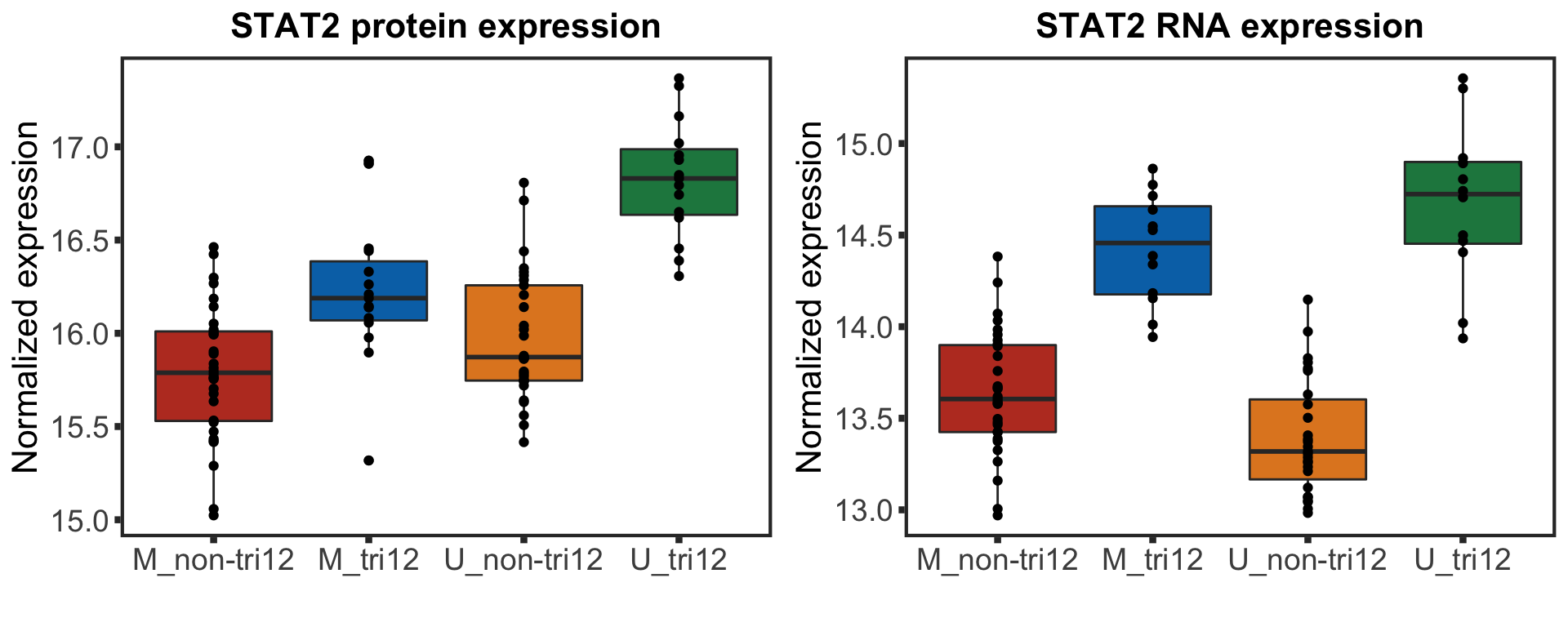

Pathway enrichment for RNA expressions correlated with STAT2 protein expression

expVar <- "STAT2"
protMat <- assays(protCLL)[["QRILC_combat"]]
rownames(protMat) <- rowData(protCLL)$hgnc_symbol
yVec <- protMat[expVar,]

Prepare data

#subset
ddsSub <- dds[,dds$PatID %in% names(yVec)]

#only keep protein coding genes with symbol
ddsSub <- ddsSub[rowData(ddsSub)$biotype %in% "protein_coding" & !rowData(ddsSub)$symbol %in% c("",NA),]

#remove lowly expressed genes
ddsSub <- ddsSub[rowSums(counts(ddsSub, normalized = TRUE)) > 100,]

#voom transformation
exprMat <- limma::voom(counts(ddsSub), lib.size = ddsSub$sizeFactor)$E
ddsSub.voom <- ddsSub
assay(ddsSub.voom) <- exprMat

rnaMat <- exprMat
rownames(rnaMat) <- rowData(ddsSub.voom)$symbol

overSampe <- intersect(names(yVec), colnames(rnaMat))

rnaMat <- rnaMat[,overSampe]
yVec <- yVec[overSampe]

Test

#buid design matirx
ighv <- patMeta[match(names(yVec),patMeta$Patient.ID),]$IGHV.status
tri12 <- patMeta[match(names(yVec),patMeta$Patient.ID),]$trisomy12

d0 <- model.matrix(~yVec)
d1 <- model.matrix(~ighv+tri12+yVec)

Without blocking for IGHV or trisomy12

fit <- lmFit(rnaMat, design = d0)
fit2 <- eBayes(fit)
resTab.noBlock <- topTable(fit2, number = Inf, coef = "yVec") %>% data.frame() %>% rownames_to_column("name")
resTab.noBlock.sig <- filter(resTab.noBlock, adj.P.Val < 0.1)

plotCorScatter <- function(plotTab, x_lab = "X", y_lab = "Y", title = "",
                           showR2 = FALSE, annoPos = "right",
                           dotCol = colList, textCol="darkred") {

  #prepare annotation values
  corRes <- cor.test(plotTab$x, plotTab$y)
  pval <- formatNum(corRes$p.value, digits = 1, format = "e")
  Rval <- formatNum(corRes$estimate, digits = 1, format = "e")
  R2val <- formatNum(corRes$estimate^2, digits = 1, format = "e")
  Nval <- nrow(plotTab)
  annoP <- bquote(italic("P")~"="~.(pval))

  if (showR2) {
    annoCoef <-  bquote(R^2~"="~.(R2val))
  } else {
    annoCoef <- bquote(R~"="~.(Rval))
  }
  annoN <- bquote(N~"="~.(Nval))

  corPlot <- ggplot(plotTab, aes(x = x, y = y)) + geom_point(aes(col = trisomy12, shape = IGHV), size=5) +
    scale_shape_manual(values = c(M = 19, U = 1)) + 
    scale_color_manual(values = c(yes = colList[2], no = colList[3])) +
    geom_smooth(formula = y~x,method = "lm", se=FALSE, color = "grey50", linetype ="dashed" ) 

  if (annoPos == "right") {

    corPlot <- corPlot + annotate("text", x = max(plotTab$x), y = Inf, label = annoN,
                                  hjust=1, vjust =2, size = 5, parse = FALSE, col= textCol) +
      annotate("text", x = max(plotTab$x), y = Inf, label = annoP,
               hjust=1, vjust =4, size = 5, parse = FALSE, col= textCol) +
      annotate("text", x = max(plotTab$x), y = Inf, label = annoCoef,
               hjust=1, vjust =6, size = 5, parse = FALSE, col= textCol)

  } else if (annoPos== "left") {
    corPlot <- corPlot + annotate("text", x = min(plotTab$x), y = Inf, label = annoN,
                                  hjust=0, vjust =2, size = 5, parse = FALSE, col= textCol) +
      annotate("text", x = min(plotTab$x), y = Inf, label = annoP,
               hjust=0, vjust =4, size = 5, parse = FALSE, col= textCol) +
      annotate("text", x = min(plotTab$x), y = Inf, label = annoCoef,
               hjust=0, vjust =6, size = 5, parse = FALSE, col= textCol)
  }
  corPlot <- corPlot + ylab(y_lab) + xlab(x_lab) + ggtitle(title) +
    scale_y_continuous(labels = scales::number_format(accuracy = 0.1)) +
    scale_x_continuous(labels = scales::number_format(accuracy = 0.1)) +
    theme_full + theme(legend.position = "bottom", plot.margin = margin(12,12,12,12))
  corPlot
}

Correlation between selected RNAs and STAT2 protein expression

geneList <- c("OAS2", "IFI44")
rnaSTAT2cor <- lapply(geneList, function(n) {
  plotTab <- tibble(x = yVec, y = rnaMat[n,], IGHV = ighv, tri12 = tri12) %>%
    mutate(trisomy12 = ifelse(tri12==1,"yes","no"))
  plotCorScatter(plotTab, annoPos = "left", x_lab = "STAT2 protein expression", y_lab = sprintf("%s RNA expression", n))
})
names(rnaSTAT2cor) <- geneList
plotRNAcor <- plot_grid(plotlist = rnaSTAT2cor)
plotRNAcor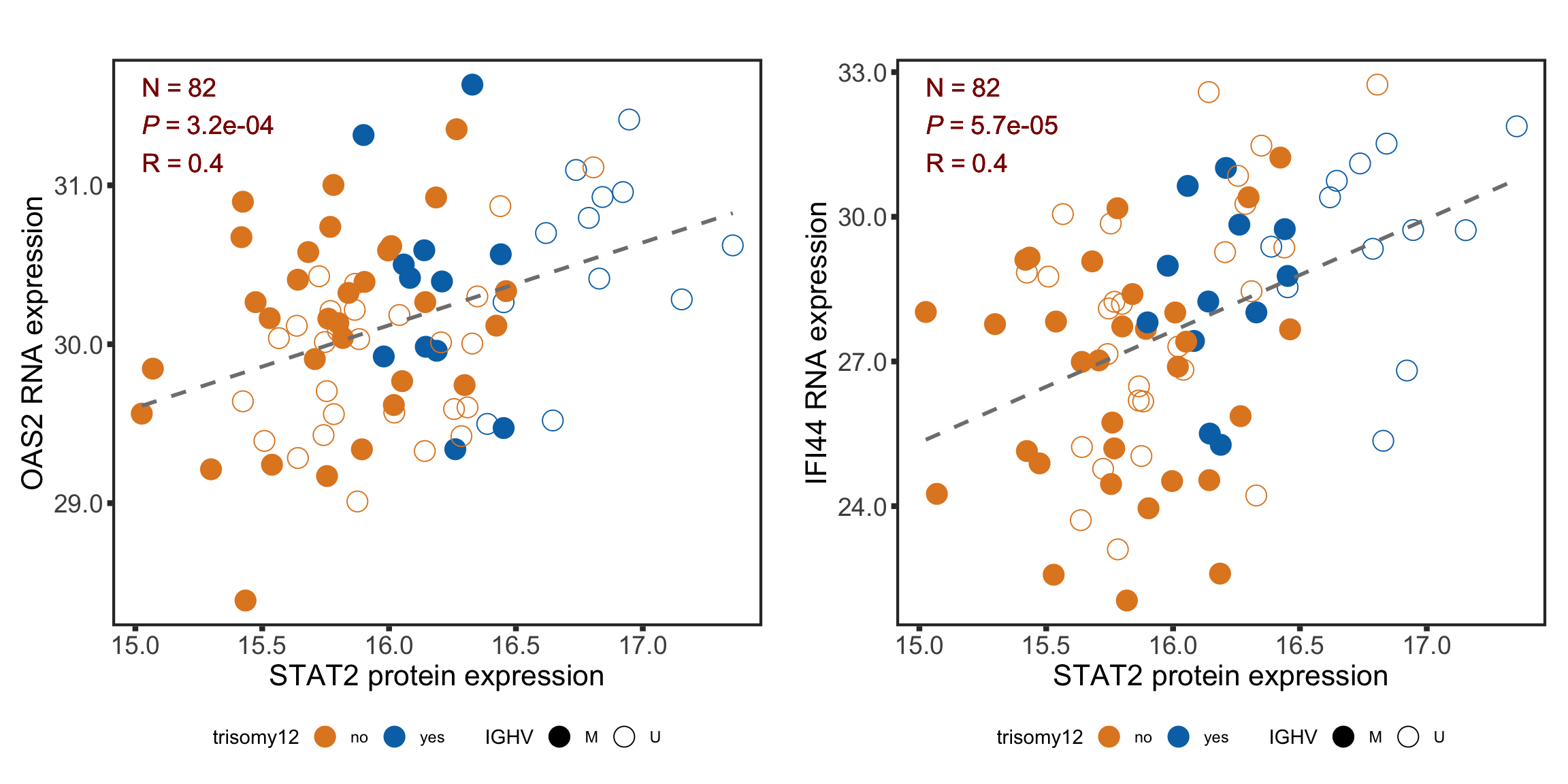

Visualize RNA expression using boxplots

geneList <- c("OAS2", "IFI44")
rnaSTAT2corBox <- lapply(geneList, function(n) {
  plotTab <- tibble(expr = rnaMat[n,], IGHV = ighv, tri12 = tri12) %>%
  mutate(trisomy12 = ifelse(tri12==1,"tri12","non-tri12")) %>%
  mutate(group = paste0(IGHV, "_", trisomy12))

ggplot(plotTab, aes(group, y=expr, fill = group)) + geom_boxplot() + geom_point() + theme_full +
  scale_fill_manual(values = colList) + theme(legend.position = "none") +
  xlab("") + ylab(sprintf("%s RNA expression",n)) + ggtitle(n)
})
names(rnaSTAT2corBox) <- geneList
plotRNAbox <- plot_grid(plotlist = rnaSTAT2corBox)
plotRNAbox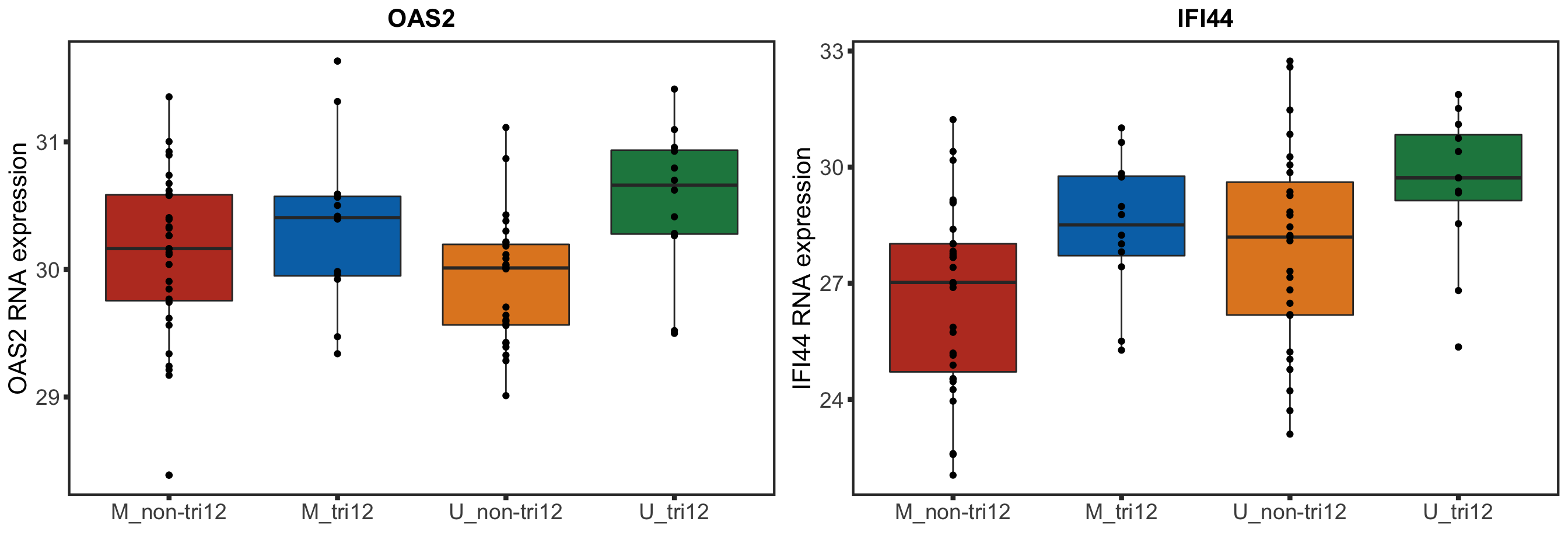

Gene enrichment analysis for RNA expressions associated with STAT2 protein expression level

gmts <- list(H = "../data/gmts/h.all.v6.2.symbols.gmt",
             KEGG = "../data/gmts/c2.cp.kegg.v6.2.symbols.gmt")

enRes <-  runCamera(rnaMat, d0, gmts$H,
            removePrefix = "HALLMARK_", pCut = 0.1, ifFDR = TRUE, setMap=setMap)
enRes$enrichPlot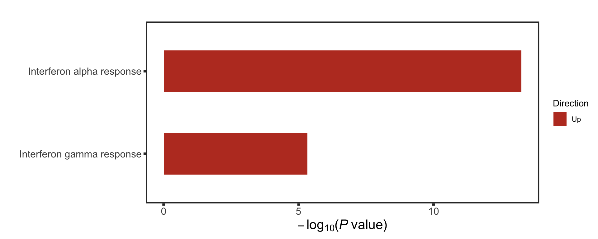

Heatmap showing the RNA expression of genes belong to the enriched pathways

colAnno <- tibble(id = names(yVec),  STAT2= yVec, IGHV = ighv, trisomy12 = tri12) %>%
  mutate(trisomy12 = ifelse(trisomy12 ==1,"yes","no")) %>%
  data.frame() %>% column_to_rownames("id")
annoCol <- list(trisomy12 = c(yes = "black",no = "grey80"),
                IGHV = c(M = colList[4], U = colList[3]),
                STAT2 = circlize::colorRamp2(c(min(colAnno$STAT2),max(colAnno$STAT2)), 
                                             c("white", "green")))

nameList <- c("STAT2","IFI44","OAS1","OAS2", "IFI30")
plotSetHeatmap(resTab.noBlock.sig, gmts$H, "HALLMARK_INTERFERON_ALPHA_RESPONSE", rnaMat, colAnno = colAnno, annoCol = annoCol, highLight = nameList)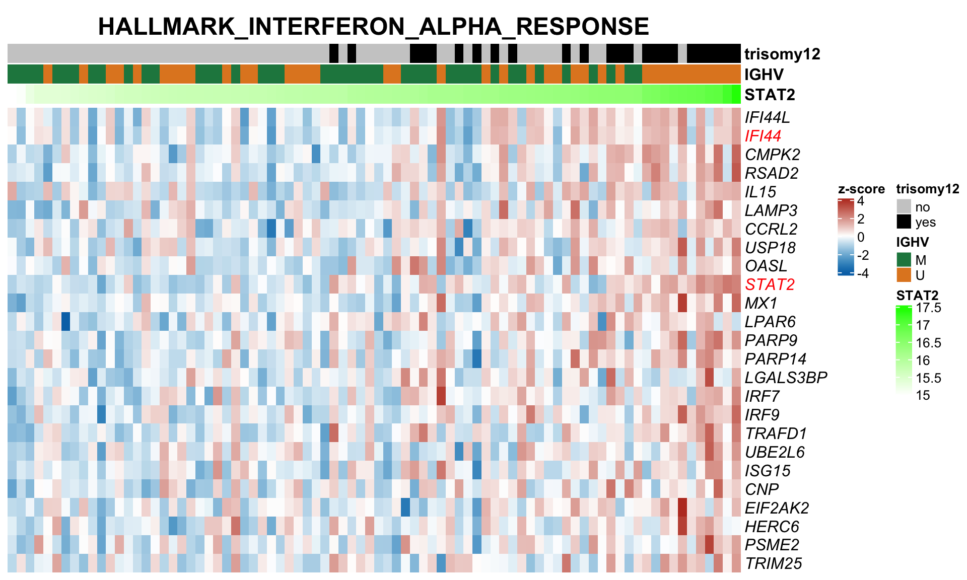

plotSetHeatmap(resTab.noBlock.sig, gmts$H, "HALLMARK_INTERFERON_GAMMA_RESPONSE", rnaMat, colAnno = colAnno, annoCol = annoCol,highLight = nameList)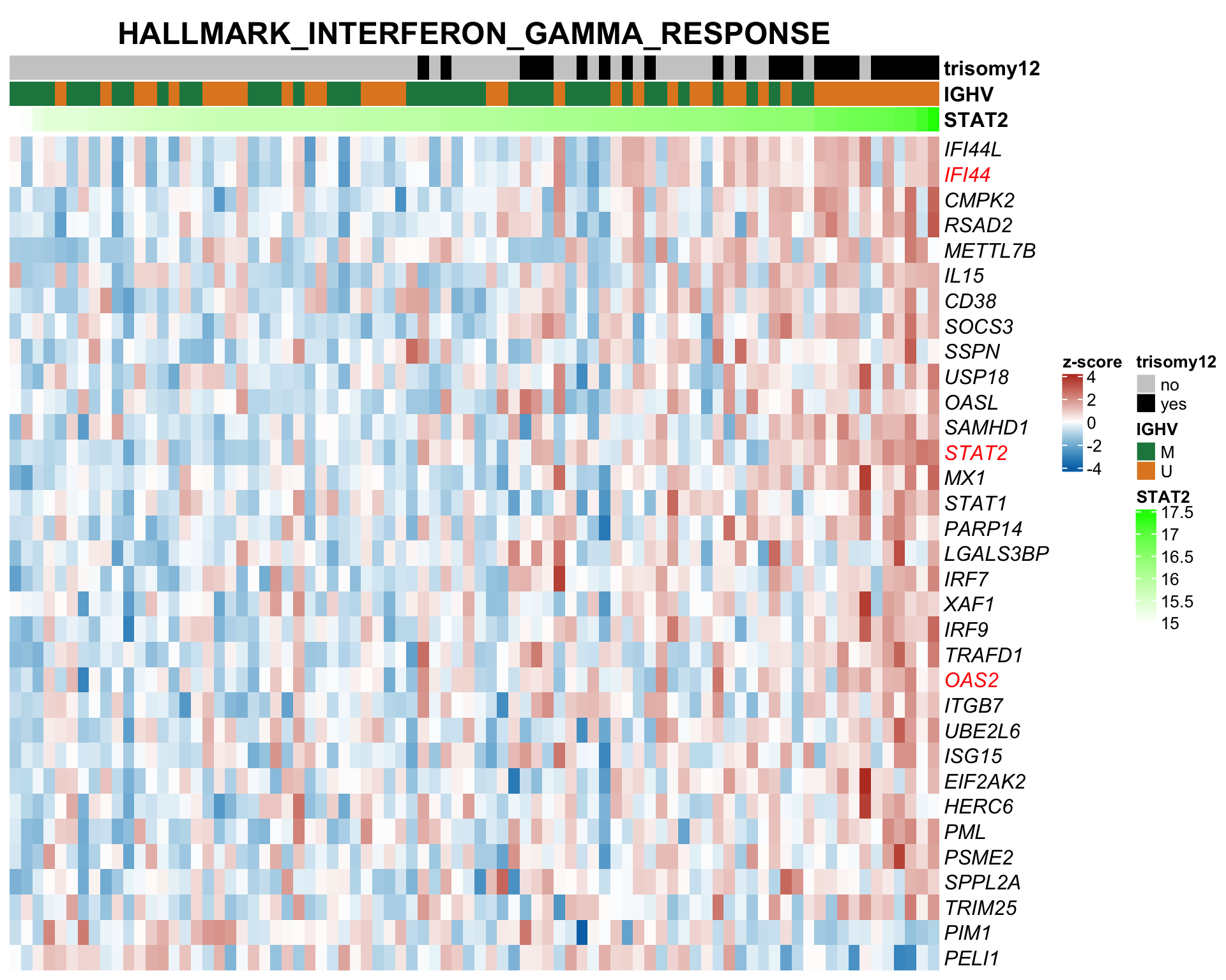

With blocking for IGHV and trisomy12

fit <- lmFit(rnaMat, design = d1)
fit2 <- eBayes(fit)
resTab.block <- topTable(fit2, number = Inf, coef = "yVec") %>% data.frame() %>% rownames_to_column("name")
resTab.block.sig <- filter(resTab.block, P.Value < 0.01)

Gene set enrichment analysis

enRes <-  runCamera(rnaMat, d1, gmts$H, contrast  = "yVec",
            removePrefix = "HALLMARK_", pCut = 0.05, ifFDR = TRUE, plotTitle = "RNA enrichment", setMap = setMap)
rnaEnrich <- enRes$enrichPlot
rnaEnrich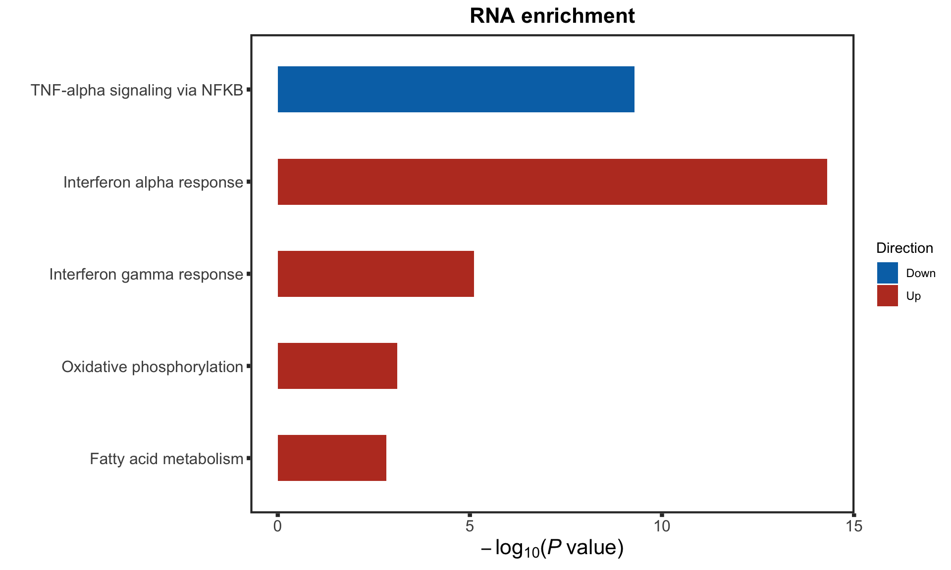

Pathway enrichment for protein expressions correlated with STAT2 protein level

Identify protein expression that are correlated with STAT2 protein expression

expVar <- "STAT2"
protMat <- assays(protCLL)[["QRILC_combat"]]
rownames(protMat) <- rowData(protCLL)$hgnc_symbol
yVec <- protMat[expVar,]
protMat <- protMat[rownames(protMat) != expVar,]

#buid design matirx
ighv <- patMeta[match(names(yVec),patMeta$Patient.ID),]$IGHV.status
tri12 <- patMeta[match(names(yVec),patMeta$Patient.ID),]$trisomy12

d0 <- model.matrix(~yVec)
d1 <- model.matrix(~ighv+tri12+yVec)

Without blocking for IGHV status and trisomy12

fit <- lmFit(protMat, design = d0)
fit2 <- eBayes(fit)
resTab.noBlock <- topTable(fit2, number = Inf, coef = "yVec") %>% data.frame() %>% mutate(name = ID)
resTab.noBlock.sig <- filter(resTab.noBlock, adj.P.Val < 0.1)

Correlation between selected proteins and STAT2 protein expression

geneList <- c("OAS1", "OAS2", "IFI30" )
geneList <- c("OAS2")

protSTAT2cor <- lapply(geneList, function(n) {
  plotTab <- tibble(x = yVec, y = protMat[n,], IGHV = ighv, tri12 = tri12) %>%
    mutate(trisomy12 = ifelse(tri12==1,"yes","no"))
  plotCorScatter(plotTab, annoPos = "left", x_lab = "STAT2 protein expression", y_lab = sprintf("%s protein expression", n)) 
})
names(protSTAT2cor) <- geneList
plot_grid(plotlist = protSTAT2cor, ncol=1)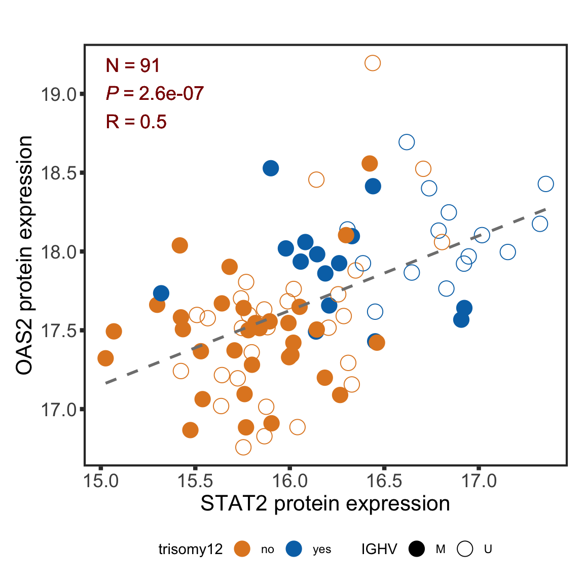

Boxplots

protSTAT2corBox <- lapply(geneList, function(n) {
  plotTab <- tibble(expr = protMat[n,], IGHV = ighv, tri12 = tri12) %>%
  mutate(trisomy12 = ifelse(tri12==1,"tri12","non-tri12")) %>%
  filter(!is.na(IGHV), !is.na(trisomy12)) %>%
  mutate(group = paste0(IGHV, "_", trisomy12))

  ggplot(plotTab, aes(group, y=expr, fill = group)) + geom_boxplot() + geom_point() + theme_full +
    scale_fill_manual(values = colList) + theme(legend.position = "none") +
    xlab("") + ylab(sprintf("%s protein expression",n)) + ggtitle(n)
})
names(protSTAT2corBox) <- geneList
plot_grid(plotlist = protSTAT2corBox, ncol=3)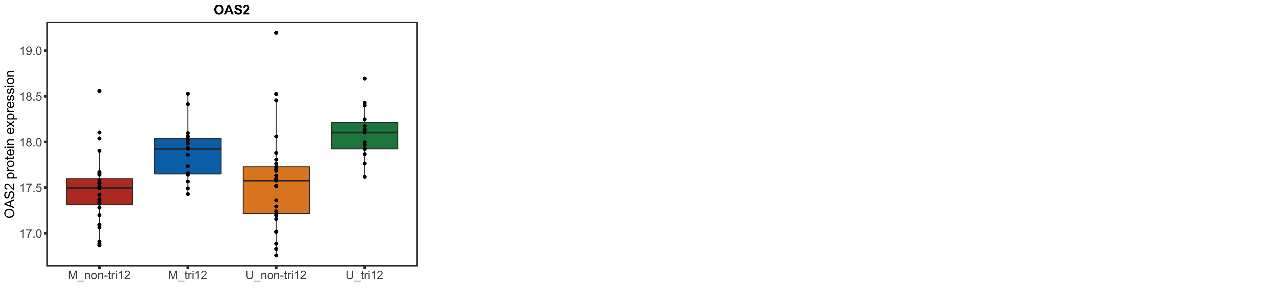

Gene set enrichment analysis

enRes <-  runCamera(protMat, d0, gmts$H,
            removePrefix = "HALLMARK_", pCut = 0.1, ifFDR = TRUE, setMap = setMap)
enRes$enrichPlot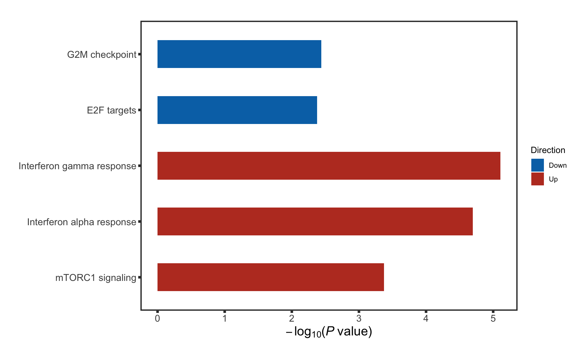

plotSetHeatmap(resTab.noBlock.sig, gmts$H, "HALLMARK_INTERFERON_ALPHA_RESPONSE", protMat, colAnno = colAnno, annoCol = annoCol, highLight = nameList)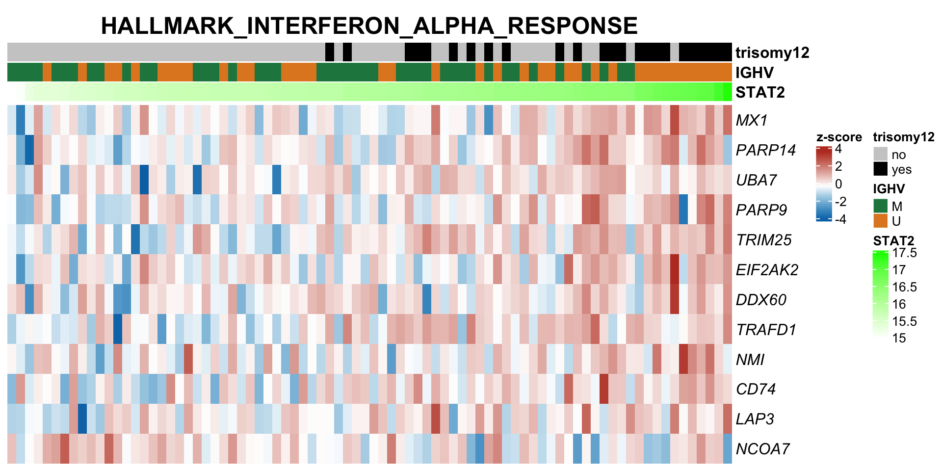

plotSetHeatmap(resTab.noBlock.sig, gmts$H, "HALLMARK_INTERFERON_GAMMA_RESPONSE", protMat, colAnno = colAnno, annoCol = annoCol, highLight = nameList)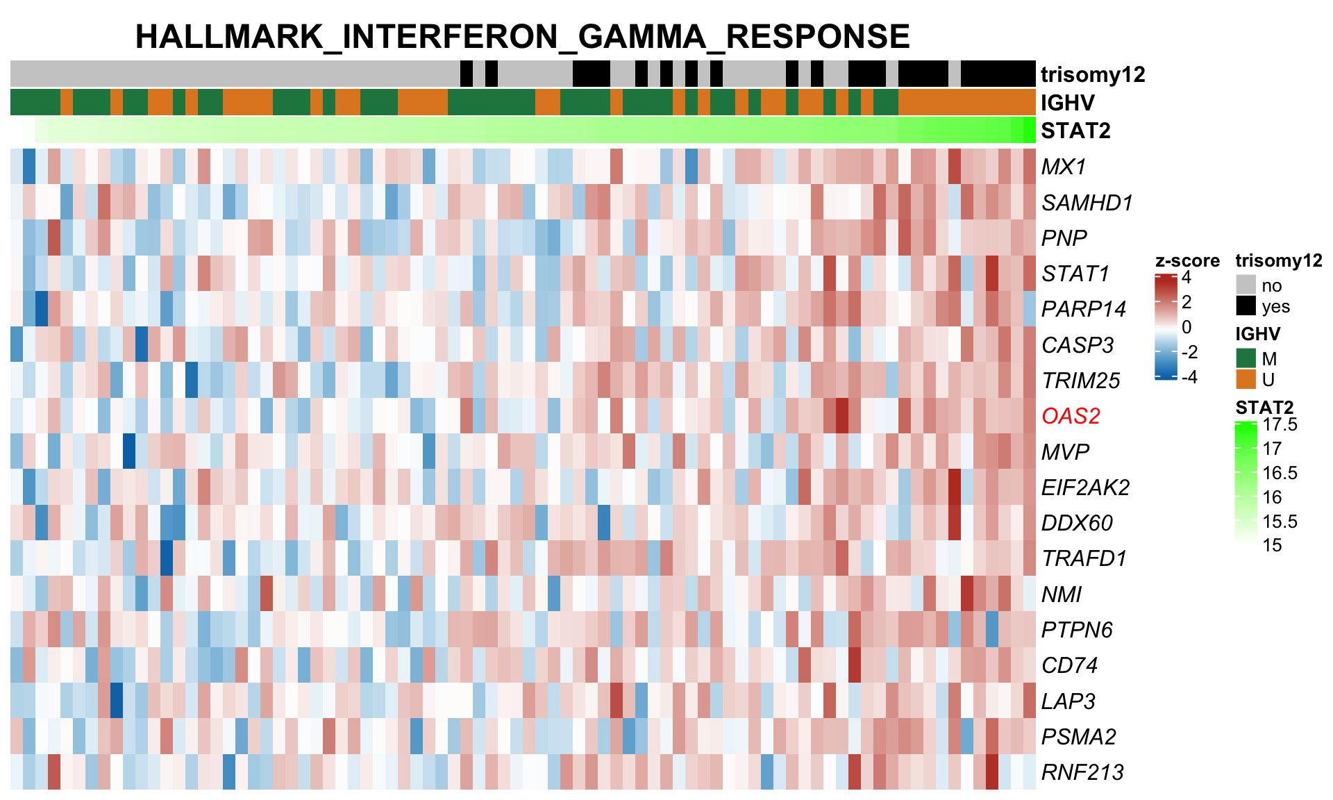

With blocking for IGHV and trisomy12

fit <- lmFit(protMat, design = d1)
fit2 <- eBayes(fit)
resTab.block <- topTable(fit2, number = Inf, coef = "yVec") %>% data.frame() %>% mutate(name=ID)
hist(resTab.block$P.Value)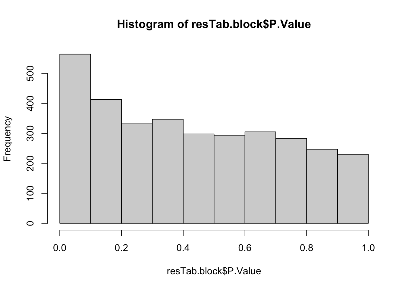

resTab.block.sig <- filter(resTab.block, P.Value < 0.01)

enRes <-  runCamera(protMat, d1, gmts$H, contrast  = "yVec",
            removePrefix = "HALLMARK_", pCut = 0.05, ifFDR = TRUE, plotTitle = "Protein enrichment", setMap = setMap)
protEnrich <- enRes$enrichPlot
protEnrich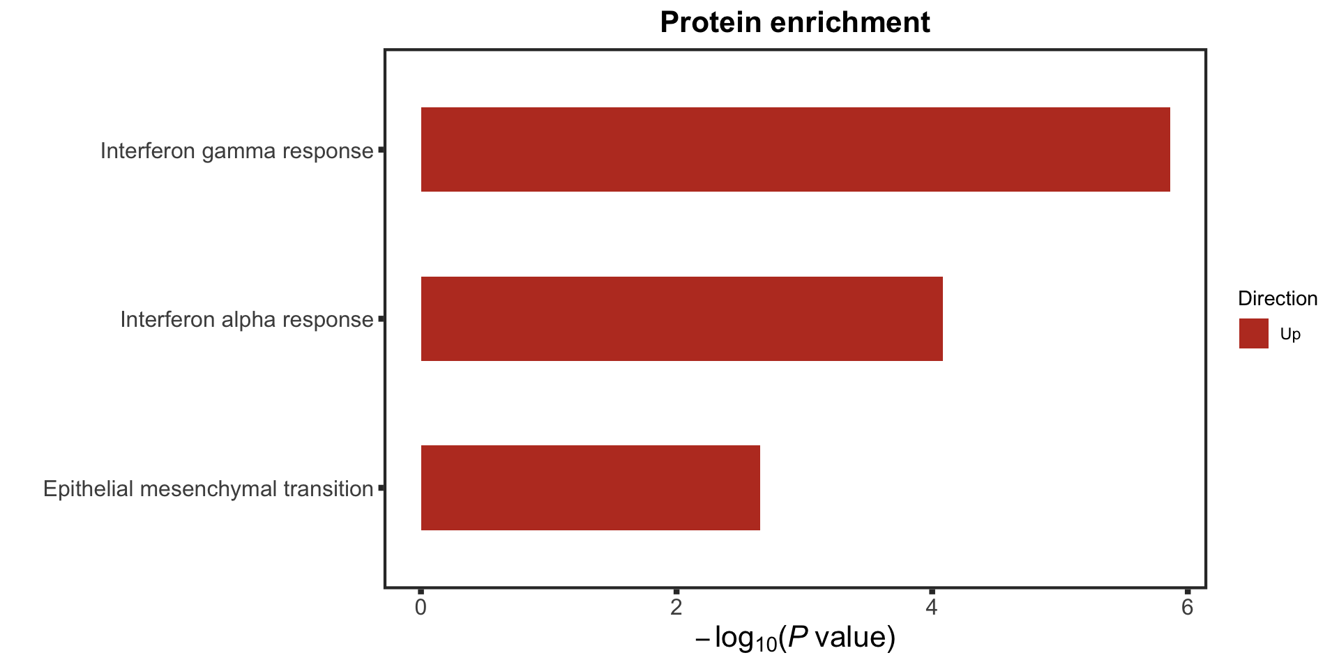

Western blot validation of STAT2 expression

Read in western results

wesTab <- readxl::read_xlsx("../data/Western_blot_results_separate_blots.xlsx") %>%
  separate(`IGHV_Tri12`, c("IGHV","trisomy12"),"_") %>%
  mutate(trisomy12 = ifelse(trisomy12 == "WT","non-tri12","tri12")) %>%
  dplyr::rename(intensity = `STAT2 Total`) %>%
  mutate(logIntensity = log10(intensity))

Associations with IGHV and trisomy12

IGHV

tRes <- car::Anova(lm(intensity~IGHV + Blot, wesTab))
pval <- tRes$`Pr(>F)`[1]

Boxplot

plotTab <- filter(wesTab) %>%
  mutate(status = ifelse(IGHV=="M","M-CLL","U-CLL")) %>%
  group_by(status) %>% mutate(n=n()) %>% ungroup() %>%
  mutate(group = sprintf("%s\n(N=%s)",status,n)) %>%
  arrange(status) %>% mutate(group = factor(group, levels = unique(group)))

pval <- formatNum(pval, digits = 2)
titleText <- bquote("STAT2 protein expression by Western Blot analysis"~" ( ANOVA "~italic("P")~"="~.(pval)~")")
pValText <-  bquote(italic("P")~"-value ="~.(pval))
ggplot(plotTab, aes(x=group, y = intensity)) +
  geom_boxplot(width=0.3, aes(fill = status), outlier.shape = NA) +
  annotate(geom = "text" ,label = pValText, x= 1.5, y=Inf, vjust=2, col = colList[1]) +
  geom_beeswarm(aes(shape = Blot), size =2.5,cex = 2, alpha=0.5) +
  ggtitle("STAT2 protein expression by Western Blot analysis")+
  #ggtitle(sprintf("%s (p = %s)",geneName, formatNum(pval, digits = 1, format = "e"))) +
  ylab("Normalized intensity") + xlab("") +
  scale_fill_manual(values = colList[3:5], name = "") +
  theme_full +
  theme(legend.position = "bottom",
        plot.title = element_text(hjust = 0.5, size=13),
        plot.margin = margin(10,10,10,10))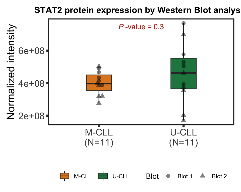

trisomy12

tRes <- car::Anova(lm(intensity~trisomy12 + Blot, wesTab))
pval <- tRes$`Pr(>F)`[1]

Boxplot

plotTab <- filter(wesTab) %>%
  mutate(status = trisomy12) %>%
  group_by(status) %>% mutate(n=n()) %>% ungroup() %>%
  mutate(group = sprintf("%s\n(N=%s)",status,n)) %>%
  arrange(status) %>% mutate(group = factor(group, levels = unique(group)))

pval <- formatNum(pval, digits = 2)
titleText <- bquote("STAT2 protein expression by Western Blot analysis"~" ( ANOVA "~italic("P")~"="~.(pval)~")")
pValText <-  bquote(italic("P")~"-value ="~.(pval))
ggplot(plotTab, aes(x=group, y = intensity)) +
  geom_boxplot(width=0.3, aes(fill = status), outlier.shape = NA) +
  annotate(geom = "text" ,label = pValText, x= 1.5, y=Inf,vjust=2, col = colList[1]) +
  geom_beeswarm(aes(shape = Blot), size =2.5,cex = 2, alpha=0.5) +
  ggtitle("STAT2 protein expression by Western Blot analysis")+
  #ggtitle(sprintf("%s (p = %s)",geneName, formatNum(pval, digits = 1, format = "e"))) +
  ylab("Normalized intensity") + xlab("") +
  scale_fill_manual(values = colList[3:5], name = "") +
  theme_full +
  theme(legend.position = "bottom",
        plot.title = element_text(hjust = 0.5, size=13),
        plot.margin = margin(10,10,10,10))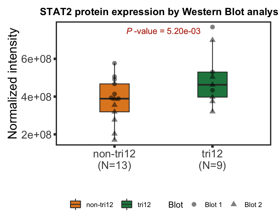

Joint IGHV and trisomy12

plotTab <- wesTab %>%
  mutate(group = paste0(IGHV, "_", trisomy12))

stat2BoxWest <- ggplot(plotTab, aes(group, y=intensity, fill = group)) + geom_boxplot() + 
  geom_beeswarm(aes(shape = Blot), size =2.5,cex = 2, alpha=0.5) +
  theme_full +
  scale_fill_manual(values = colList, name = "") + theme(legend.position = "bottom") +
  xlab("") + ggtitle("STAT2 protein expression by Western Blot analysis") +ylab("Normalized intensity")

stat2BoxWest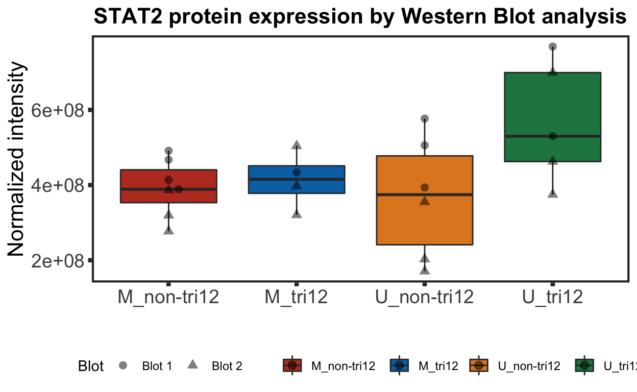

Analysis of the PCR results of CLL cell lines with and without STAT2 knockouts

Load datasets

tab1 <- readxl::read_xlsx("../data/CAS9results.xlsx", sheet = 1) %>% mutate(control = "ACTB") 
tab2 <- readxl::read_xlsx("../data/CAS9results.xlsx", sheet = 2) %>% mutate(control = "GAPDH")
pcrTab <- bind_rows(tab1, tab2) %>% separate(name, into = c("cellLine","sgRNA","treatment","IFN"), sep = "[_ ]", remove = FALSE) %>%
  pivot_longer(contains("fold change"), names_to = "replicate",values_to = "foldChange") %>%
  mutate(replicate=str_replace(replicate, "fold change replicate ","R"),
         IFN = ifelse(treatment == "+", "IFN", "no IFN"),
         trisomy12 = ifelse(cellLine %in% c("MEC-1","HG-3"), "no" ,"yes"),
         sgTreat= paste0(sgRNA," ",treatment," IFN")) %>%
  select(-treatment) %>%
  mutate(sgRNA = factor(sgRNA, levels = c("NTC","34A","36D")),
         Gene = factor(Gene, levels = c("STAT2","OAS1","OAS2"))) %>%
  arrange(sgRNA, Gene) %>%
  mutate(sgTreat = factor(sgTreat, levels = unique(sgTreat))) %>%
  mutate(log2foldChange = log2(foldChange))
geneSymbol <- c(bquote(italic("STAT2")),bquote(italic("OAS1")), bquote(italic("OAS2")))

GAPDH as control

plotTab <- pcrTab %>% filter(control == "GAPDH")

barGAPDH <- ggplot(plotTab, aes(x=sgTreat, y=log2foldChange)) +
  geom_bar(aes(fill = Gene), position = "dodge", stat = "summary", fun.y = "mean") +
  geom_point(aes(dodge=Gene), col = "black", position = position_dodge(width = 0.9)) +
  scale_fill_manual(values = colList, labels = geneSymbol) +
  facet_wrap(~cellLine, scale = "free_x", ncol=2 ) +
  xlab("") + ylab(bquote("log"[2]*"(fold change) relative to control in RNA expression")) +
  #scale_y_continuous() +
  geom_hline(yintercept = 0, linetype = "dashed", col = "grey50") +
  theme_half +
  theme(axis.text.x = element_text(angle = 90, hjust=1, vjust=0.5),
        strip.text = element_text(size=12, face= "bold"),
        legend.position = "right")
barGAPDH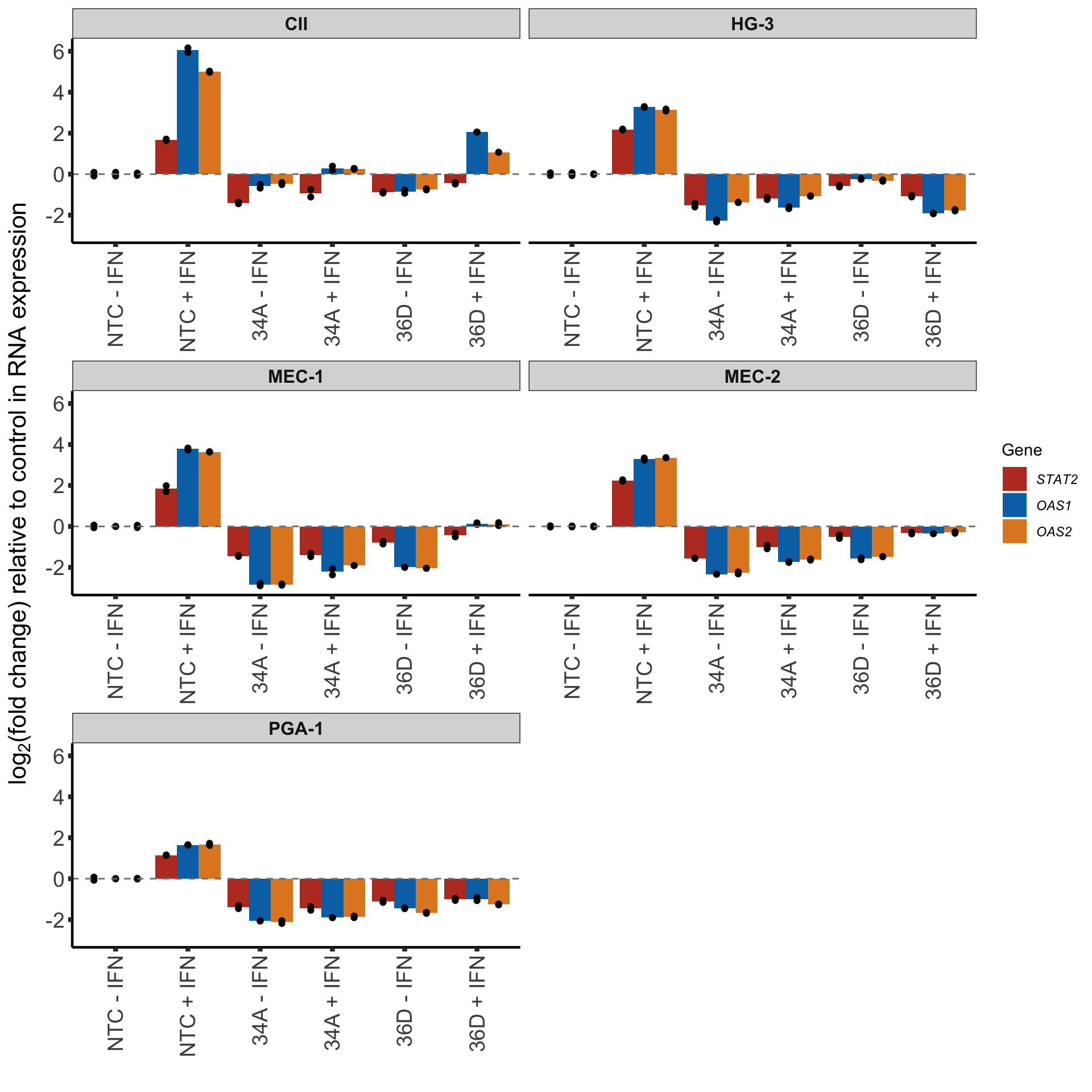

ACTB as control

plotTab <- pcrTab %>% filter(control == "ACTB")

barACTB <- ggplot(plotTab, aes(x=sgTreat, y=log2foldChange)) +
  geom_bar(aes(fill = Gene), position = "dodge", stat = "summary", fun.y = "mean") +
  geom_point(aes(dodge=Gene), col = "black", position = position_dodge(width = 0.9)) +
  scale_fill_manual(values = colList, labels = geneSymbol) +
  facet_wrap(~cellLine, scale = "free_x", ncol=2) +
  xlab("") + ylab(bquote("log"[2]*"(fold change) relative to control in RNA expression")) +
  #scale_y_continuous() +
  geom_hline(yintercept = 0, linetype = "dashed", col = "grey50") +
  theme_half +
  theme(axis.text.x = element_text(angle = 90, hjust=1, vjust=0.5),
        strip.text = element_text(size=12, face= "bold"),
        legend.position = "right")
barACTB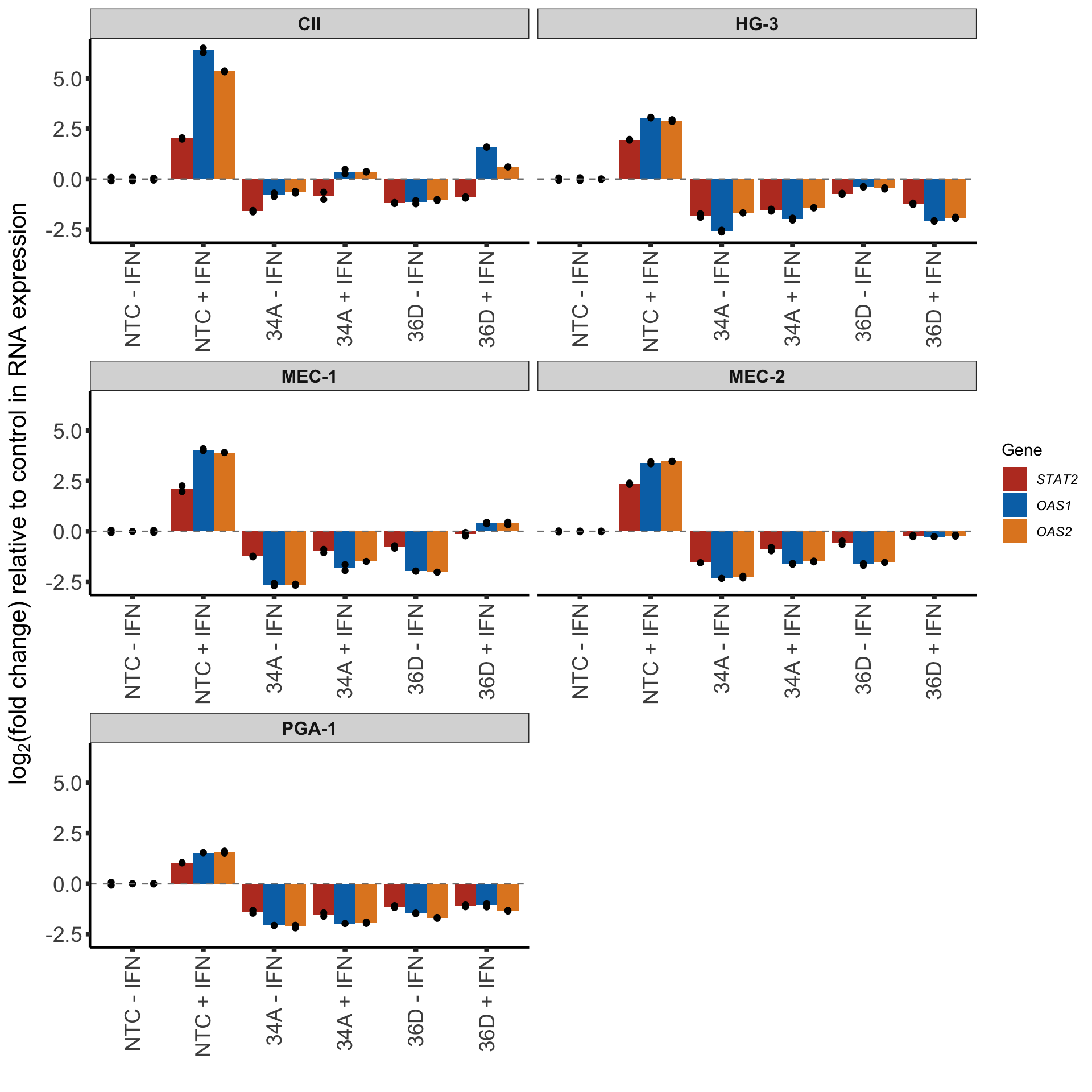

Compare trisomy12 cell lines with non-trisomy12 cell lines

pcrTab <- readxl::read_excel("../data/STATexprPCR.xlsx") %>%
  separate(name, into = c("cellLine", "sgRNA","IFN","other"),sep = " ") %>%
  #mutate(IFN = ifelse(IFN == "+","with ","no ")) %>%
  mutate(IFN = paste0(IFN, " ",other),
         trisomy12 = str_replace(trisomy12, "Non","non")) %>% 
  arrange( trisomy12, IFN) %>%
  mutate(group = paste0(trisomy12," ", IFN)) %>%
  mutate(group =factor(group, levels=unique(group)),
         sgRNA = factor(sgRNA, levels = c("NTC","34A","36D")),
         Gene = factor(Gene, levels = c("STAT2","OAS1","OAS2"))) %>%
  group_by(cellLine, sgRNA, group, Gene) %>%
  summarise(fc = mean(foldChange)) %>%
  ungroup()

geneSymbol <- c(bquote(italic("STAT2")),bquote(italic("OAS1")), bquote(italic("OAS2")))


meanTab <- group_by(pcrTab, group, sgRNA, Gene) %>%
  summarise(meanVal = mean(fc))
  
ggplot(pcrTab, aes(x=group, y = fc, col = Gene, group = Gene)) +
  geom_point(aes(shape = cellLine),position = position_dodge(width = 0.8), size=3) +
  xlab("") + ylab("fold change") +
  #ggrepel::geom_text_repel(aes(label = cellLine)) +
  scale_color_manual(values = colList, labels = geneSymbol, name = "gene") +
  scale_shape_discrete(name = "cell line") +
  geom_point(data=meanTab, aes(x=group, y=meanVal), position = position_dodge(width = 0.8), color= "grey50", shape = "—", size=6) +
  #scale_y_continuous(limits = c(-3,6)) +
  #ggtitle(sprintf("%s expression (%s)", geneName, condi)) +
  facet_wrap(~sgRNA, ncol=3, scale = "free_x") +
  theme_full + theme(legend.position = "right",
                     plot.title = element_text(face = "bold"),
                     strip.text = element_text(size=12), 
                     axis.text.x = element_text(angle = 45, hjust=1, vjust=1))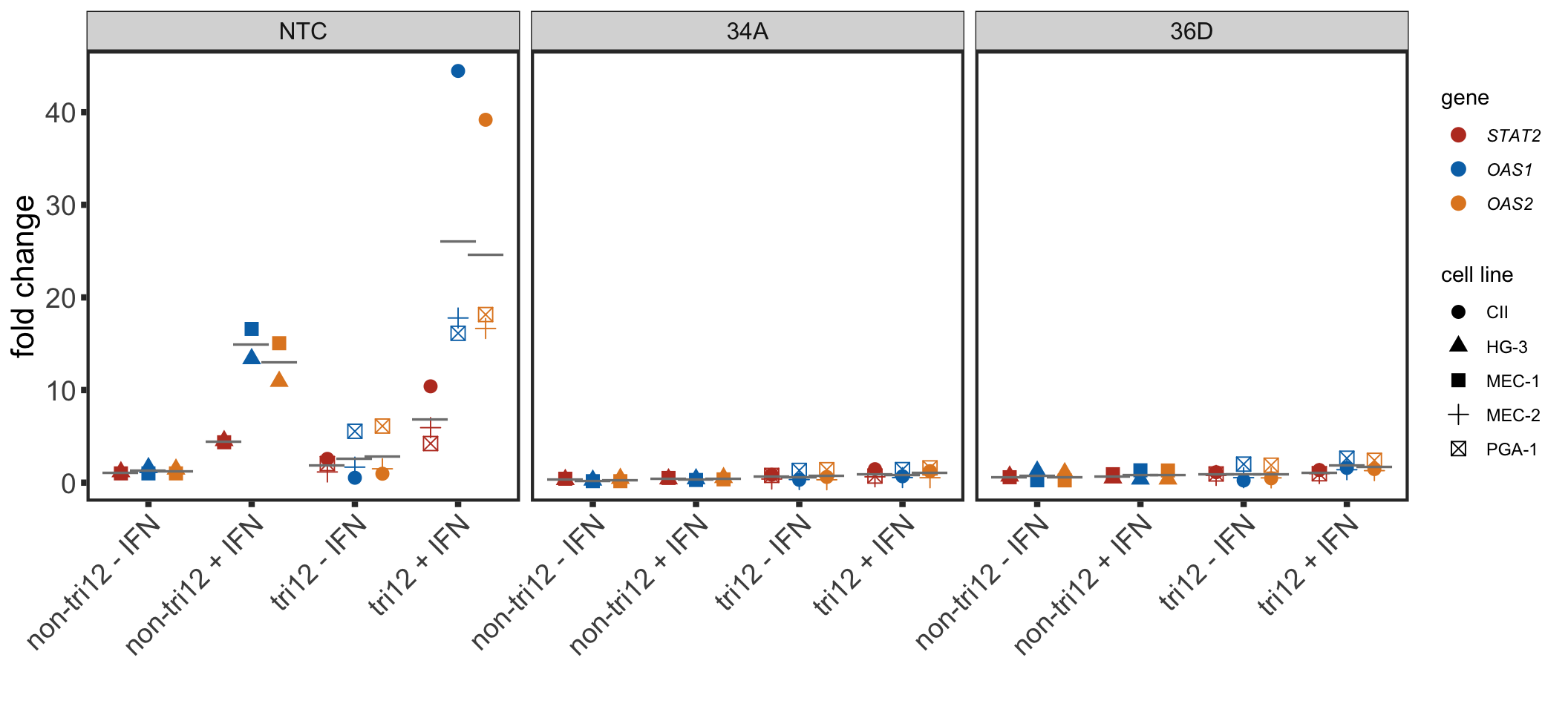

sessionInfo()

R version 4.0.2 (2020-06-22)
Platform: x86_64-apple-darwin17.0 (64-bit)
Running under: macOS  10.16

Matrix products: default
BLAS:   /Library/Frameworks/R.framework/Versions/4.0/Resources/lib/libRblas.dylib
LAPACK: /Library/Frameworks/R.framework/Versions/4.0/Resources/lib/libRlapack.dylib

locale:
[1] en_US.UTF-8/en_US.UTF-8/en_US.UTF-8/C/en_US.UTF-8/en_US.UTF-8

attached base packages:
 [1] parallel  stats4    grid      stats     graphics  grDevices utils    
 [8] datasets  methods   base     

other attached packages:
 [1] DESeq2_1.28.1               latex2exp_0.4.0            
 [3] forcats_0.5.1               stringr_1.4.0              
 [5] dplyr_1.0.5                 purrr_0.3.4                
 [7] readr_1.4.0                 tidyr_1.1.3                
 [9] tibble_3.1.0                tidyverse_1.3.0            
[11] SummarizedExperiment_1.18.2 DelayedArray_0.14.1        
[13] matrixStats_0.58.0          Biobase_2.48.0             
[15] GenomicRanges_1.40.0        GenomeInfoDb_1.24.2        
[17] IRanges_2.22.2              S4Vectors_0.26.1           
[19] BiocGenerics_0.34.0         glmnet_4.1-1               
[21] Matrix_1.3-2                ggbeeswarm_0.6.0           
[23] ggplot2_3.3.3               gtable_0.3.0               
[25] limma_3.44.3                jyluMisc_0.1.5             
[27] ComplexHeatmap_2.4.3        pheatmap_1.0.12            
[29] piano_2.4.0                 cowplot_1.1.1              

loaded via a namespace (and not attached):
  [1] utf8_1.1.4             shinydashboard_0.7.1   tidyselect_1.1.0      
  [4] RSQLite_2.2.3          AnnotationDbi_1.50.3   htmlwidgets_1.5.3     
  [7] BiocParallel_1.22.0    maxstat_0.7-25         munsell_0.5.0         
 [10] codetools_0.2-18       DT_0.17                withr_2.4.1           
 [13] colorspace_2.0-0       highr_0.8              knitr_1.31            
 [16] rstudioapi_0.13        ggsignif_0.6.1         labeling_0.4.2        
 [19] git2r_0.28.0           slam_0.1-48            GenomeInfoDbData_1.2.3
 [22] KMsurv_0.1-5           bit64_4.0.5            farver_2.1.0          
 [25] rprojroot_2.0.2        vctrs_0.3.6            generics_0.1.0        
 [28] TH.data_1.0-10         xfun_0.21              sets_1.0-18           
 [31] R6_2.5.0               clue_0.3-58            locfit_1.5-9.4        
 [34] cachem_1.0.4           bitops_1.0-6           fgsea_1.14.0          
 [37] assertthat_0.2.1       promises_1.2.0.1       scales_1.1.1          
 [40] multcomp_1.4-16        beeswarm_0.3.1         egg_0.4.5             
 [43] sandwich_3.0-0         workflowr_1.6.2        rlang_0.4.10          
 [46] genefilter_1.70.0      GlobalOptions_0.1.2    splines_4.0.2         
 [49] rstatix_0.7.0          broom_0.7.5            yaml_2.2.1            
 [52] abind_1.4-5            modelr_0.1.8           backports_1.2.1       
 [55] httpuv_1.5.5           tools_4.0.2            relations_0.6-9       
 [58] ellipsis_0.3.1         gplots_3.1.1           jquerylib_0.1.3       
 [61] RColorBrewer_1.1-2     Rcpp_1.0.6             visNetwork_2.0.9      
 [64] zlibbioc_1.34.0        RCurl_1.98-1.2         ggpubr_0.4.0          
 [67] GetoptLong_1.0.5       zoo_1.8-9              haven_2.3.1           
 [70] cluster_2.1.1          exactRankTests_0.8-31  fs_1.5.0              
 [73] magrittr_2.0.1         data.table_1.14.0      openxlsx_4.2.3        
 [76] circlize_0.4.12        reprex_1.0.0           survminer_0.4.9       
 [79] mvtnorm_1.1-1          hms_1.0.0              shinyjs_2.0.0         
 [82] mime_0.10              evaluate_0.14          xtable_1.8-4          
 [85] XML_3.99-0.5           rio_0.5.26             readxl_1.3.1          
 [88] gridExtra_2.3          shape_1.4.5            compiler_4.0.2        
 [91] KernSmooth_2.23-18     crayon_1.4.1           htmltools_0.5.1.1     
 [94] mgcv_1.8-34            later_1.1.0.1          geneplotter_1.66.0    
 [97] lubridate_1.7.10       DBI_1.1.1              dbplyr_2.1.0          
[100] MASS_7.3-53.1          car_3.0-10             cli_2.3.1             
[103] marray_1.66.0          igraph_1.2.6           pkgconfig_2.0.3       
[106] km.ci_0.5-2            foreign_0.8-81         xml2_1.3.2            
[109] foreach_1.5.1          annotate_1.66.0        vipor_0.4.5           
[112] bslib_0.2.4            XVector_0.28.0         drc_3.0-1             
[115] rvest_1.0.0            digest_0.6.27          rmarkdown_2.7         
[118] cellranger_1.1.0       fastmatch_1.1-0        survMisc_0.5.5        
[121] curl_4.3               shiny_1.6.0            gtools_3.8.2          
[124] rjson_0.2.20           nlme_3.1-152           lifecycle_1.0.0       
[127] jsonlite_1.7.2         carData_3.0-4          fansi_0.4.2           
[130] pillar_1.5.1           lattice_0.20-41        fastmap_1.1.0         
[133] httr_1.4.2             plotrix_3.8-1          survival_3.2-7        
[136] glue_1.4.2             zip_2.1.1              png_0.1-7             
[139] iterators_1.0.13       bit_4.0.4              stringi_1.5.3         
[142] sass_0.3.1             blob_1.2.1             memoise_2.0.0         
[145] caTools_1.18.1

Section 9: Explaining STAT2 protein expression using multi-omic data

Junyan Lu

2020-10-09

Load packages and datasets

Feature selection with LASSO on multi-omic data to explain STAT2 protein expression

Preprocessing multi-omic data

Feature selection with LASSO (L1) penalty

Variance explained for STAT2 expression by multi-omics datasets

Heatmap of selected features

Genetics only

Combined

LASSO model with only protein and RNA combined

IGHV mutational status and trisomy12 status jointly determine STAT2 protein expression

ANOVA test on IGHV/trisomy12 status to STAT2 protein expression

ANOVA test on IGHV/trisomy12 status to STAT2 RNA expression

Visualize differences using boxplots

Pathway enrichment for RNA expressions correlated with STAT2 protein expression

Without blocking for IGHV or trisomy12

Correlation between selected RNAs and STAT2 protein expression

Gene enrichment analysis for RNA expressions associated with STAT2 protein expression level

Heatmap showing the RNA expression of genes belong to the enriched pathways

With blocking for IGHV and trisomy12

Pathway enrichment for protein expressions correlated with STAT2 protein level

Identify protein expression that are correlated with STAT2 protein expression

Without blocking for IGHV status and trisomy12

Correlation between selected proteins and STAT2 protein expression

Gene set enrichment analysis

With blocking for IGHV and trisomy12

Western blot validation of STAT2 expression

Associations with IGHV and trisomy12

IGHV

trisomy12

Analysis of the PCR results of CLL cell lines with and without STAT2 knockouts

Compare trisomy12 cell lines with non-trisomy12 cell lines