Last updated: 2022-11-17

Checks: 5 1

Knit directory: LungCancer_SotilloLab/analysis/

This reproducible R Markdown analysis was created with workflowr (version 1.7.0). The Checks tab describes the reproducibility checks that were applied when the results were created. The Past versions tab lists the development history.

Environment: empty

Great job! The global environment was empty. Objects defined in the global environment can affect the analysis in your R Markdown file in unknown ways. For reproduciblity it’s best to always run the code in an empty environment.

Seed: set.seed(20221103)

The command set.seed(20221103) was run prior to running the code in the R Markdown file. Setting a seed ensures that any results that rely on randomness, e.g. subsampling or permutations, are reproducible.

Session information: recorded

Great job! Recording the operating system, R version, and package versions is critical for reproducibility.

Cache: none

Nice! There were no cached chunks for this analysis, so you can be confident that you successfully produced the results during this run.

File paths: relative

Great job! Using relative paths to the files within your workflowr project makes it easier to run your code on other machines.

Repository version: no version control

Tracking code development and connecting the code version to the results is critical for reproducibility. To start using Git, open the Terminal and type git init in your project directory.

This project is not being versioned with Git. To obtain the full reproducibility benefits of using workflowr, please see ?wflow_start.

Load packages and dataset

#package
library(SummarizedExperiment)
library(MultiAssayExperiment)
library(proDA)
library(tidyverse)
source("../code/utils.R")
knitr::opts_chunk$set(warning = FALSE, message = FALSE, autodep = TRUE)

Load processed data

load("../output/processedData.RData")

Phosphoproteomic

Preprocessing

Use different normalization method

#variance stabilizing normalization
ppe.vst <- preprocessPhos(maeData, missCut = 0.5, transform = "vst")

[1] "Number of proteins and samples:"
[1] 3787   96

#log2 + median normalization
ppe.log2Med <- preprocessPhos(maeData, missCut = 0.5, transform = "log2", normalize = TRUE)

[1] "Number of proteins and samples:"
[1] 3787   96

#only log2 transformation
ppe.log2Only <- preprocessPhos(maeData, missCut = 0.5, transform ="log2", normalize = FALSE)

[1] "Number of proteins and samples:"
[1] 3787   96

#log2 transformation + normalization based on precursur quantity
ppe.pre <- preprocessPhos(maeData, missCut = 0.5, transform ="log2", normalize = TRUE, usePrecursor = TRUE)

[1] "Number of proteins and samples:"
[1] 3787   96

Mean SD plots

VST

vsn::meanSdPlot(assay(ppe.vst))

Log2+median

vsn::meanSdPlot(assay(ppe.log2Med))

log2 only

vsn::meanSdPlot(assay(ppe.log2Only))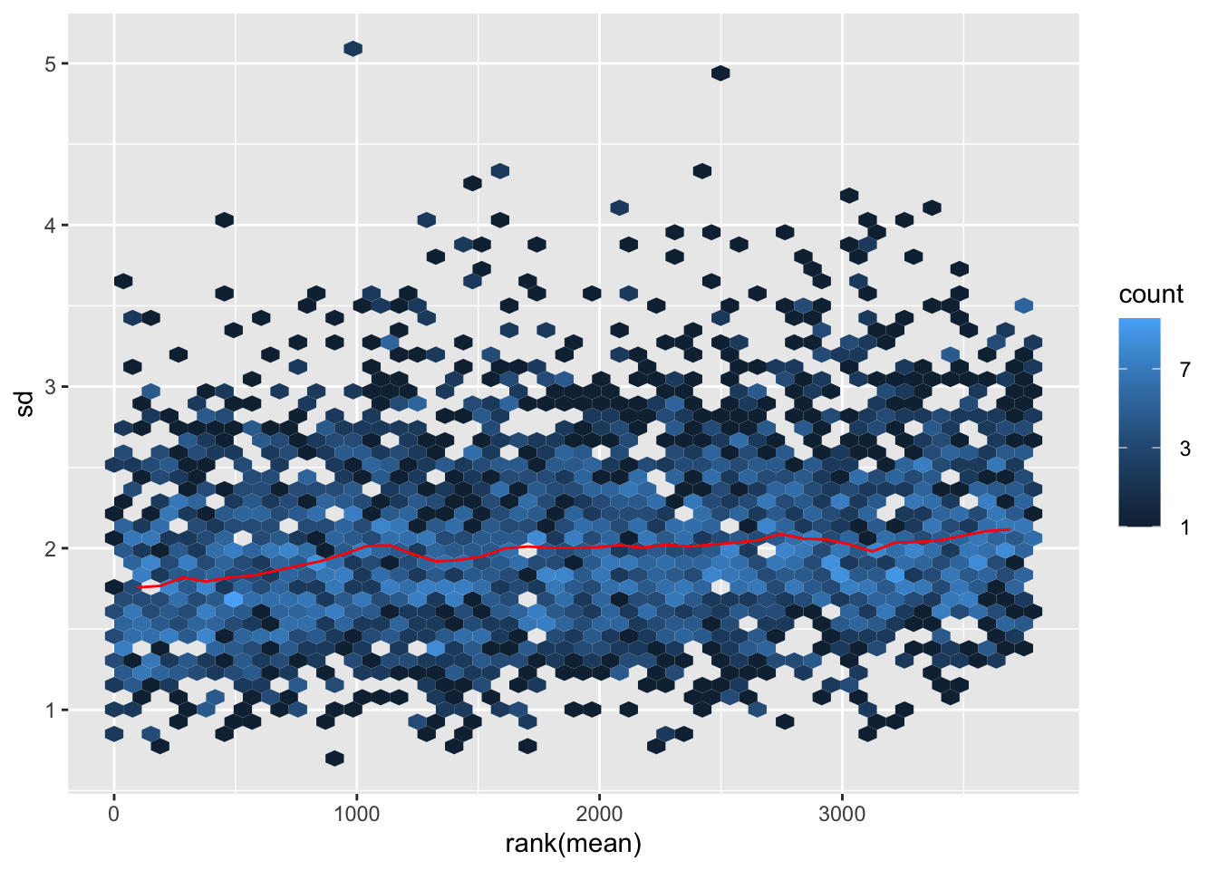

#### Use precursor

vsn::meanSdPlot(assay(ppe.pre))

Distribution after normalization

VST

countMat <- assay(ppe.vst)
annoTab <- colData(ppe.vst)[,c("sample","time","drug")] %>% as_tibble()
countTab <- countMat %>% as_tibble(rownames = "id") %>% 
    pivot_longer(-id) %>%
    filter(!is.na(value)) %>%
    left_join(annoTab, by = c(name = "sample"))
ggplot(countTab, aes(x=name, y=value)) +
    geom_boxplot(aes(fill = time)) +
    facet_wrap(~drug, scales = "free_x") +
    theme(axis.text.x = element_text(angle = 90, hjust = 1, vjust = 0.5))

log2+median

countMat <- assay(ppe.log2Med)
annoTab <- colData(ppe.log2Med)[,c("sample","time","drug")] %>% as_tibble()
countTab <- countMat %>% as_tibble(rownames = "id") %>% 
    pivot_longer(-id) %>%
    filter(!is.na(value)) %>%
    left_join(annoTab, by = c(name = "sample"))
ggplot(countTab, aes(x=name, y=value)) +
    geom_boxplot(aes(fill = time)) +
    facet_wrap(~drug, scales = "free_x") +
    theme(axis.text.x = element_text(angle = 90, hjust = 1, vjust = 0.5))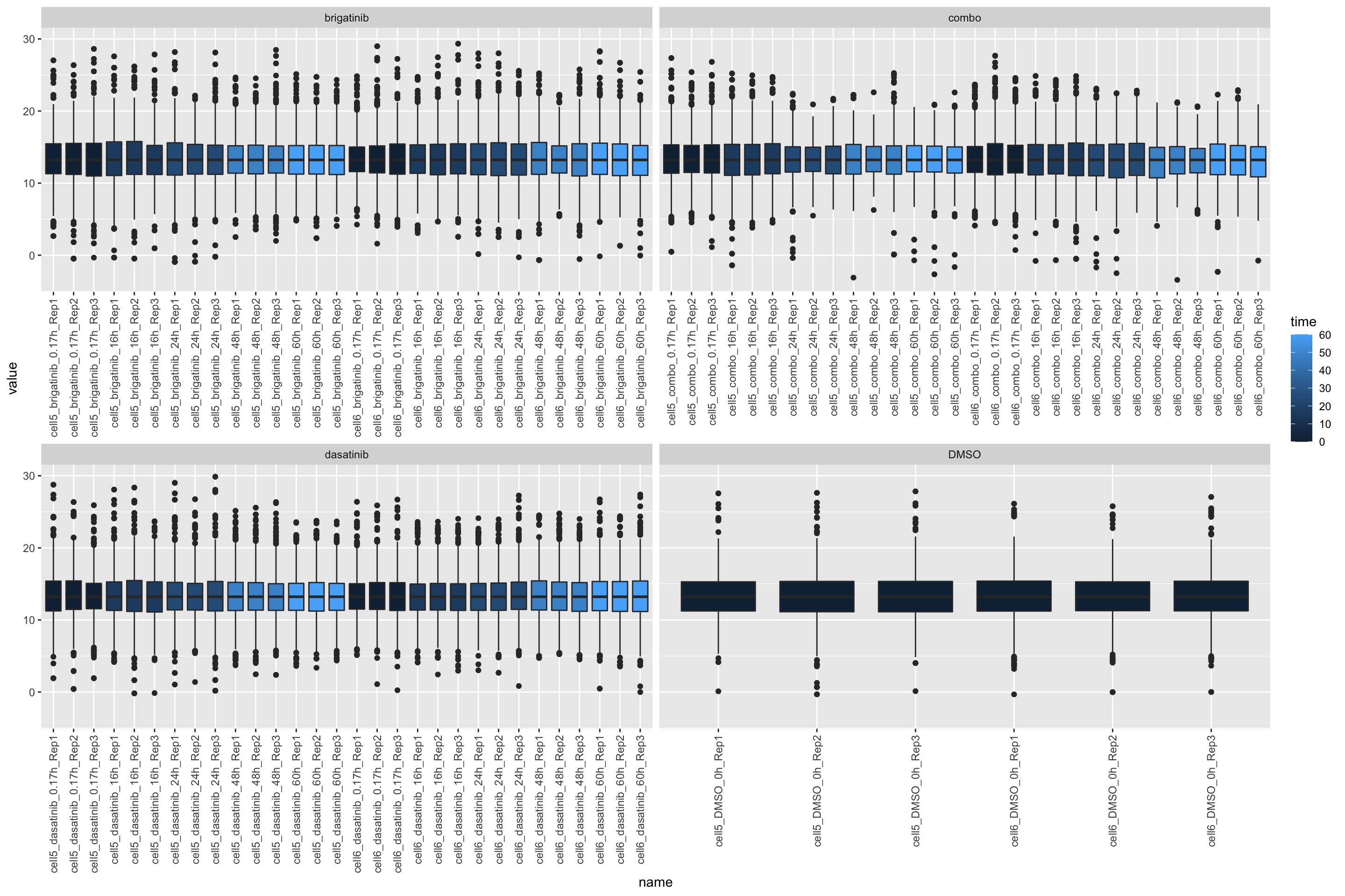

#### only transformation

countMat <- assay(ppe.log2Only)
annoTab <- colData(ppe.log2Only)[,c("sample","time","drug")] %>% as_tibble()
countTab <- countMat %>% as_tibble(rownames = "id") %>% 
    pivot_longer(-id) %>%
    filter(!is.na(value)) %>%
    left_join(annoTab, by = c(name = "sample"))
ggplot(countTab, aes(x=name, y=value)) +
    geom_boxplot(aes(fill = time)) +
    facet_wrap(~drug, scales = "free_x") +
    theme(axis.text.x = element_text(angle = 90, hjust = 1, vjust = 0.5))

use precursor

countMat <- assay(ppe.pre)
annoTab <- colData(ppe.pre)[,c("sample","time","drug")] %>% as_tibble()
countTab <- countMat %>% as_tibble(rownames = "id") %>% 
    pivot_longer(-id) %>%
    filter(!is.na(value)) %>%
    left_join(annoTab, by = c(name = "sample"))
ggplot(countTab, aes(x=name, y=value)) +
    geom_boxplot(aes(fill = time)) +
    facet_wrap(~drug, scales = "free_x") +
    theme(axis.text.x = element_text(angle = 90, hjust = 1, vjust = 0.5))

PCA

VST

exprMat <- assays(ppe.vst)[["imputed"]]
sds <- genefilter::rowSds(exprMat)
exprMat <- exprMat[order(sds, decreasing = TRUE)[1:2000],]

smpAnno <- colData(ppe.vst) %>%
    as_tibble(rownames = "id")

pcRes <- prcomp(t(exprMat), scale. = TRUE, center = TRUE)
pcTab <- pcRes$x[,1:10] %>% 
    as_tibble(rownames = "id") %>%
    left_join(smpAnno)

PC1 versus PC2

ggplot(pcTab, aes(x=PC1, y=PC2)) +
    geom_point(aes(col = drug, size = factor(time),
               shape = replicate)) +
    ggrepel::geom_text_repel(aes(label = id)) +
    theme_bw()

PC3 versus PC4

ggplot(pcTab, aes(x=PC3, y=PC4)) +
        geom_point(aes(col = drug, size = factor(time),
               shape = replicate)) +
    ggrepel::geom_text_repel(aes(label = id)) +
    theme_bw()

log2+median

exprMat <- assays(ppe.log2Med)[["imputed"]]
sds <- genefilter::rowSds(exprMat)
exprMat <- exprMat[order(sds, decreasing = TRUE)[1:2000],]

smpAnno <- colData(ppe.log2Med) %>%
    as_tibble(rownames = "id")

pcRes <- prcomp(t(exprMat), scale. = TRUE, center = TRUE)
pcTab <- pcRes$x[,1:10] %>% 
    as_tibble(rownames = "id") %>%
    left_join(smpAnno)

PC1 versus PC2

ggplot(pcTab, aes(x=PC1, y=PC2)) +
    geom_point(aes(col = drug, size = factor(time),
               shape = replicate)) +
    ggrepel::geom_text_repel(aes(label = id)) +
    theme_bw()

PC3 versus PC4

ggplot(pcTab, aes(x=PC3, y=PC4)) +
        geom_point(aes(col = drug, size = factor(time),
               shape = replicate)) +
    ggrepel::geom_text_repel(aes(label = id)) +
    theme_bw()

log2 only

exprMat <- assays(ppe.log2Only)[["imputed"]]
sds <- genefilter::rowSds(exprMat)
exprMat <- exprMat[order(sds, decreasing = TRUE)[1:2000],]

smpAnno <- colData(ppe.log2Only) %>%
    as_tibble(rownames = "id")

pcRes <- prcomp(t(exprMat), scale. = TRUE, center = TRUE)
pcTab <- pcRes$x[,1:10] %>% 
    as_tibble(rownames = "id") %>%
    left_join(smpAnno)

PC1 versus PC2

ggplot(pcTab, aes(x=PC1, y=PC2)) +
    geom_point(aes(col = drug, size = factor(time),
               shape = replicate)) +
    ggrepel::geom_text_repel(aes(label = id)) +
    theme_bw()

PC3 versus PC4

ggplot(pcTab, aes(x=PC3, y=PC4)) +
        geom_point(aes(col = drug, size = factor(time),
               shape = replicate)) +
    ggrepel::geom_text_repel(aes(label = id)) +
    theme_bw()

Use precursor

exprMat <- assays(ppe.pre)[["imputed"]]
sds <- genefilter::rowSds(exprMat)
exprMat <- exprMat[order(sds, decreasing = TRUE)[1:2000],]

smpAnno <- colData(ppe.pre) %>%
    as_tibble(rownames = "id")

pcRes <- prcomp(t(exprMat), scale. = TRUE, center = TRUE)
pcTab <- pcRes$x[,1:10] %>% 
    as_tibble(rownames = "id") %>%
    left_join(smpAnno)

PC1 versus PC2

ggplot(pcTab, aes(x=PC1, y=PC2)) +
    geom_point(aes(col = drug, size = factor(time),
               shape = replicate)) +
    ggrepel::geom_text_repel(aes(label = id)) +
    theme_bw()

PC3 versus PC4

ggplot(pcTab, aes(x=PC3, y=PC4)) +
        geom_point(aes(col = drug, size = factor(time),
               shape = replicate)) +
    ggrepel::geom_text_repel(aes(label = id)) +
    theme_bw()

Hierarchical clustering

VST

colAnno <- colData(ppe.vst)[,c("cellLine","drug","time")] %>% data.frame()
exprMat.scaled <- jyluMisc::mscale(exprMat, center = TRUE, scale = TRUE, censor = 5)
pheatmap::pheatmap(exprMat.scaled, annotation_col = colAnno, clustering_method = "ward.D2",
                   color = colorRampPalette(c("blue","white","red"))(100), 
                   breaks = seq(-5,5, length.out = 101), 
                   show_rownames = FALSE)

log2+median

colAnno <- colData(ppe.log2Med)[,c("cellLine","drug","time")] %>% data.frame()
exprMat.scaled <- jyluMisc::mscale(exprMat, center = TRUE, scale = TRUE, censor = 5)
pheatmap::pheatmap(exprMat.scaled, annotation_col = colAnno, clustering_method = "ward.D2",
                   color = colorRampPalette(c("blue","white","red"))(100), 
                   breaks = seq(-5,5, length.out = 101), 
                   show_rownames = FALSE)

log2 only

colAnno <- colData(ppe.log2Only)[,c("cellLine","drug","time")] %>% data.frame()
exprMat.scaled <- jyluMisc::mscale(exprMat, center = TRUE, scale = TRUE, censor = 5)
pheatmap::pheatmap(exprMat.scaled, annotation_col = colAnno, clustering_method = "ward.D2",
                   color = colorRampPalette(c("blue","white","red"))(100), 
                   breaks = seq(-5,5, length.out = 101), 
                   show_rownames = FALSE)

precursor

colAnno <- colData(ppe.pre)[,c("cellLine","drug","time")] %>% data.frame()
exprMat.scaled <- jyluMisc::mscale(exprMat, center = TRUE, scale = TRUE, censor = 5)
pheatmap::pheatmap(exprMat.scaled, annotation_col = colAnno, clustering_method = "ward.D2",
                   color = colorRampPalette(c("blue","white","red"))(100), 
                   breaks = seq(-5,5, length.out = 101), 
                   show_rownames = FALSE)

Remove one potential outlier

maeSub <- maeData[, maeData$sample != "cell5_combo_24h_Rep2"]

#variance stabilizing normalization
ppe.vst <- preprocessPhos(maeSub, missCut = 0.5, transform = "vst")

[1] "Number of proteins and samples:"
[1] 3879   95

#log2 + median normalization
ppe.log2Med <- preprocessPhos(maeSub, missCut = 0.5, transform = "log2", normalize = TRUE)

[1] "Number of proteins and samples:"
[1] 3879   95

#only log2 transformation
ppe.log2Only <- preprocessPhos(maeSub, missCut = 0.5, transform ="log2", normalize = FALSE)

[1] "Number of proteins and samples:"
[1] 3879   95

#log2 transformation + normalization based on precursur quantity
ppe.pre <- preprocessPhos(maeData, missCut = 0.5, transform ="log2", normalize = TRUE, usePrecursor = TRUE)

[1] "Number of proteins and samples:"
[1] 3787   96

PCA

VST

exprMat <- assays(ppe.vst)[["imputed"]]
sds <- genefilter::rowSds(exprMat)
exprMat <- exprMat[order(sds, decreasing = TRUE)[1:2000],]

smpAnno <- colData(ppe.vst) %>%
    as_tibble(rownames = "id")

pcRes <- prcomp(t(exprMat), scale. = TRUE, center = TRUE)
pcTab <- pcRes$x[,1:10] %>% 
    as_tibble(rownames = "id") %>%
    left_join(smpAnno)

PC1 versus PC2

ggplot(pcTab, aes(x=PC1, y=PC2)) +
    geom_point(aes(col = drug, size = factor(time),
               shape = replicate)) +
    ggrepel::geom_text_repel(aes(label = id)) +
    theme_bw()

PC3 versus PC4

ggplot(pcTab, aes(x=PC3, y=PC4)) +
        geom_point(aes(col = drug, size = factor(time),
               shape = replicate)) +
    ggrepel::geom_text_repel(aes(label = id)) +
    theme_bw()

log2+median

exprMat <- assays(ppe.log2Med)[["imputed"]]
sds <- genefilter::rowSds(exprMat)
exprMat <- exprMat[order(sds, decreasing = TRUE)[1:2000],]

smpAnno <- colData(ppe.log2Med) %>%
    as_tibble(rownames = "id")

pcRes <- prcomp(t(exprMat), scale. = TRUE, center = TRUE)
pcTab <- pcRes$x[,1:10] %>% 
    as_tibble(rownames = "id") %>%
    left_join(smpAnno)

PC1 versus PC2

ggplot(pcTab, aes(x=PC1, y=PC2)) +
    geom_point(aes(col = drug, size = factor(time),
               shape = replicate)) +
    ggrepel::geom_text_repel(aes(label = id)) +
    theme_bw()

PC3 versus PC4

ggplot(pcTab, aes(x=PC3, y=PC4)) +
        geom_point(aes(col = drug, size = factor(time),
               shape = replicate)) +
    ggrepel::geom_text_repel(aes(label = id)) +
    theme_bw()

log2 only

exprMat <- assays(ppe.log2Only)[["imputed"]]
sds <- genefilter::rowSds(exprMat)
exprMat <- exprMat[order(sds, decreasing = TRUE)[1:2000],]

smpAnno <- colData(ppe.log2Only) %>%
    as_tibble(rownames = "id")

pcRes <- prcomp(t(exprMat), scale. = TRUE, center = TRUE)
pcTab <- pcRes$x[,1:10] %>% 
    as_tibble(rownames = "id") %>%
    left_join(smpAnno)

PC1 versus PC2

ggplot(pcTab, aes(x=PC1, y=PC2)) +
    geom_point(aes(col = drug, size = factor(time),
               shape = replicate)) +
    ggrepel::geom_text_repel(aes(label = id)) +
    theme_bw()

PC3 versus PC4

ggplot(pcTab, aes(x=PC3, y=PC4)) +
        geom_point(aes(col = drug, size = factor(time),
               shape = replicate)) +
    ggrepel::geom_text_repel(aes(label = id)) +
    theme_bw()

Use precursor

exprMat <- assays(ppe.pre)[["imputed"]]
sds <- genefilter::rowSds(exprMat)
exprMat <- exprMat[order(sds, decreasing = TRUE)[1:2000],]

smpAnno <- colData(ppe.pre) %>%
    as_tibble(rownames = "id")

pcRes <- prcomp(t(exprMat), scale. = TRUE, center = TRUE)
pcTab <- pcRes$x[,1:10] %>% 
    as_tibble(rownames = "id") %>%
    left_join(smpAnno)

PC1 versus PC2

ggplot(pcTab, aes(x=PC1, y=PC2)) +
    geom_point(aes(col = drug, size = factor(time),
               shape = replicate)) +
    ggrepel::geom_text_repel(aes(label = id)) +
    theme_bw()

PC3 versus PC4

ggplot(pcTab, aes(x=PC3, y=PC4)) +
        geom_point(aes(col = drug, size = factor(time),
               shape = replicate)) +
    ggrepel::geom_text_repel(aes(label = id)) +
    theme_bw()

Hierarchical clustering

VST

colAnno <- colData(ppe.vst)[,c("cellLine","drug","time")] %>% data.frame()
exprMat.scaled <- jyluMisc::mscale(exprMat, center = TRUE, scale = TRUE, censor = 5)
pheatmap::pheatmap(exprMat.scaled, annotation_col = colAnno, clustering_method = "ward.D2",
                   color = colorRampPalette(c("blue","white","red"))(100), 
                   breaks = seq(-5,5, length.out = 101), 
                   show_rownames = FALSE)

log2+median

colAnno <- colData(ppe.log2Med)[,c("cellLine","drug","time")] %>% data.frame()
exprMat.scaled <- jyluMisc::mscale(exprMat, center = TRUE, scale = TRUE, censor = 5)
pheatmap::pheatmap(exprMat.scaled, annotation_col = colAnno, clustering_method = "ward.D2",
                   color = colorRampPalette(c("blue","white","red"))(100), 
                   breaks = seq(-5,5, length.out = 101), 
                   show_rownames = FALSE)

log2 only

colAnno <- colData(ppe.log2Only)[,c("cellLine","drug","time")] %>% data.frame()
exprMat.scaled <- jyluMisc::mscale(exprMat, center = TRUE, scale = TRUE, censor = 5)
pheatmap::pheatmap(exprMat.scaled, annotation_col = colAnno, clustering_method = "ward.D2",
                   color = colorRampPalette(c("blue","white","red"))(100), 
                   breaks = seq(-5,5, length.out = 101), 
                   show_rownames = FALSE)

precursor

colAnno <- colData(ppe.pre)[,c("cellLine","drug","time")] %>% data.frame()
exprMat.scaled <- jyluMisc::mscale(exprMat, center = TRUE, scale = TRUE, censor = 5)
pheatmap::pheatmap(exprMat.scaled, annotation_col = colAnno, clustering_method = "ward.D2",
                   color = colorRampPalette(c("blue","white","red"))(100), 
                   breaks = seq(-5,5, length.out = 101), 
                   show_rownames = FALSE)

Compare the reproducibiliy of replicates when using different normalization methods

Function to calculate reproducibility of replicates

getSdTab <- function(x) {
  sd <- jyluMisc::sumToTidy(x) %>%
  group_by(sampleCondi, rowID) %>%
  summarise(sdVal = sd(Intensity,na.rm=TRUE), meanVal = mean(Intensity,na.rm=TRUE)) %>%
  filter(!is.na(sdVal)) %>% mutate(meanRnk = order(meanVal))
}

sdTab.vst <- getSdTab(ppe.vst) %>% mutate(norm = "vst")
sdTab.log2Med <- getSdTab(ppe.log2Med) %>% mutate(norm = "log2Med")
sdTab.log2Only <- getSdTab(ppe.log2Only) %>% mutate(norm = "log2Only")
sdTab.pre <- getSdTab(ppe.pre) %>% mutate(norm = "precursor")
sumTab <- bind_rows(sdTab.vst, sdTab.log2Med, sdTab.log2Only, sdTab.pre)

Add annotations

colTab <- colData(ppe.vst) %>% as_tibble() %>%
  distinct(sampleCondi,.keep_all = TRUE)
sumTab <- left_join(sumTab, colTab)

Overall distribution

ggplot(sumTab, aes(x=sdVal, fill = norm)) +
  geom_histogram(position = "identity", alpha=0.5, color = "grey50") +
  xlim(0,6)

Per sample

ggplot(sumTab, aes(x=sampleCondi, y = sdVal, fill = norm)) +
  geom_violin() +
  facet_wrap(~drug, scale="free_x")+
  theme(axis.text.x = element_text(angle = 90, hjust = 1, vjust = 0.5))

Mean versus SD

ggplot(sumTab, aes(x=meanVal, y=sdVal)) +
  geom_hex() + geom_smooth()  +
  facet_wrap(~norm, ncol=1)

Rank of sd for each normalization method

ordTab <- group_by(sumTab, sampleCondi, rowID) %>%
  mutate(index = order(sdVal))
ggplot(ordTab, aes(x=index, fill = norm)) +
  geom_bar(position = "dodge", alpha=0.5, color = "grey50")

For each sample, which normalization method gives the best reproduciblity for replicates

ordPerTab <- arrange(ordTab, index) %>% distinct(sampleCondi, drug,.keep_all = TRUE) %>%
  group_by(sampleCondi, norm, drug) %>% summarise(n=length(rowID))
ggplot(ordPerTab, aes(x=sampleCondi, y = n, fill = norm)) +
  geom_bar(stat="identity")+
  facet_wrap(~drug, scale = "free_x") +
  theme(axis.text.x = element_text(angle = 90, hjust = 1, vjust = 0.5))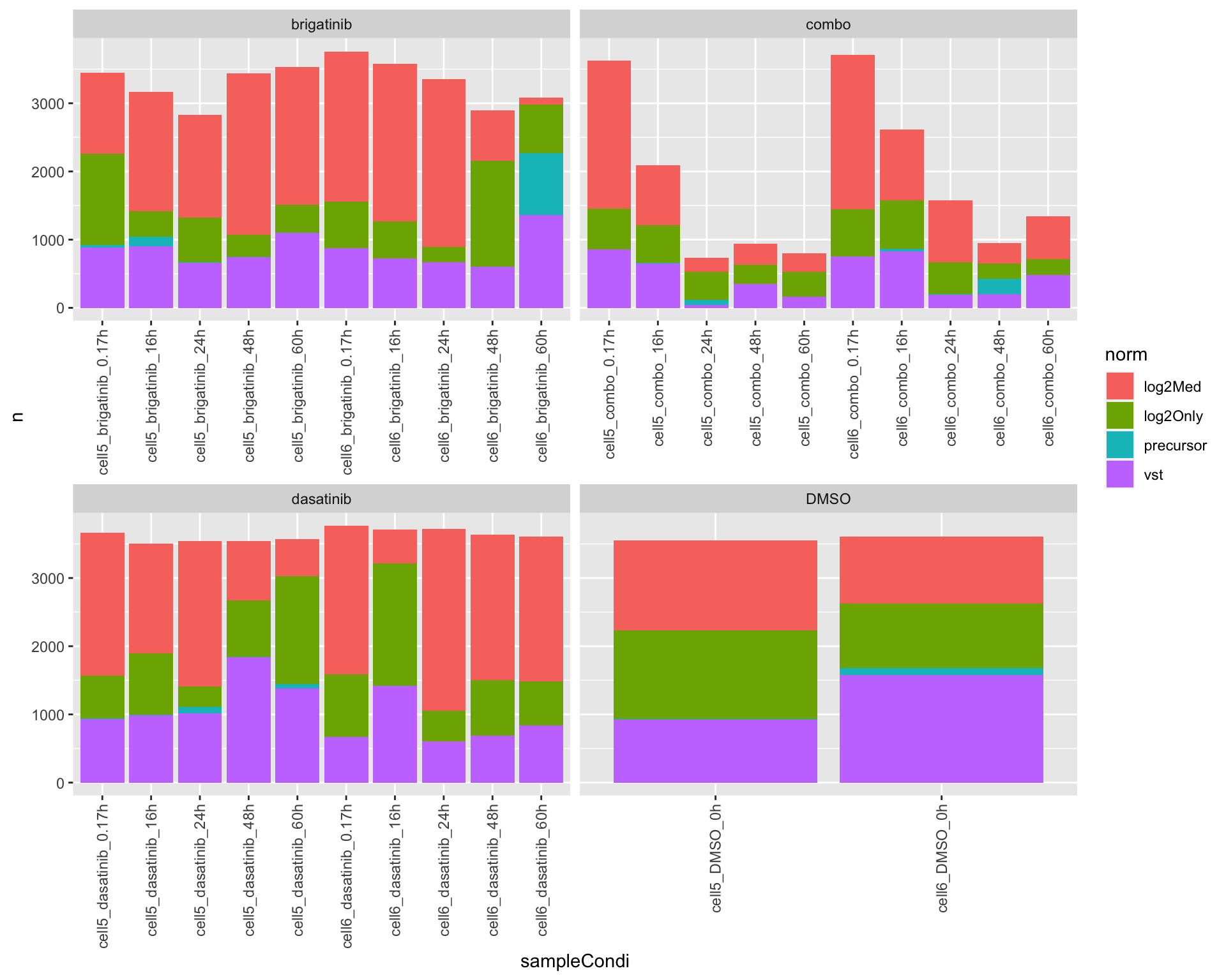

It seems log2 + median scaling can get the best reproducibility among replicates. No normalization is the worst.

Proteomic

Preprocessing

Use different normalization method

#variance stabilizing normalization
ppe.vst <- preprocessProteome(maeData, missCut = 0.5, transform = "vst")

[1] "Number of proteins and samples:"
[1] 7608   96

#log2 + median normalization
ppe.log2Med <- preprocessProteome(maeData, missCut = 0.5, transform = "log2", normalize = TRUE)

[1] "Number of proteins and samples:"
[1] 7608   96

#only log2 transformation
ppe.log2Only <- preprocessProteome(maeData, missCut = 0.5, transform ="log2", normalize = FALSE)

[1] "Number of proteins and samples:"
[1] 7608   96

#log2 transformation + normalization based on precursur quantity
ppe.pre <- preprocessProteome(maeData, missCut = 0.5, transform ="log2", normalize = TRUE, usePrecursor = TRUE)

[1] "Number of proteins and samples:"
[1] 7608   96

Mean SD plots

VST

vsn::meanSdPlot(assay(ppe.vst))

Log2+median

vsn::meanSdPlot(assay(ppe.log2Med))

log2 only

vsn::meanSdPlot(assay(ppe.log2Only))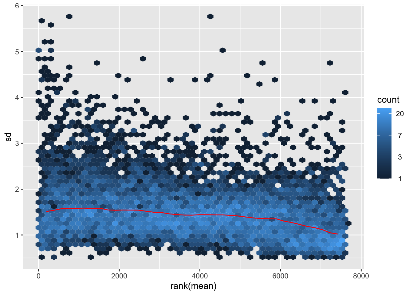

#### Use precursor

vsn::meanSdPlot(assay(ppe.pre))

Distribution after normalization

VST

countMat <- assay(ppe.vst)
annoTab <- colData(ppe.vst)[,c("sample","time","drug")] %>% as_tibble()
countTab <- countMat %>% as_tibble(rownames = "id") %>% 
    pivot_longer(-id) %>%
    filter(!is.na(value)) %>%
    left_join(annoTab, by = c(name = "sample"))
ggplot(countTab, aes(x=name, y=value)) +
    geom_boxplot(aes(fill = time)) +
    facet_wrap(~drug, scales = "free_x") +
    theme(axis.text.x = element_text(angle = 90, hjust = 1, vjust = 0.5))

log2+median

countMat <- assay(ppe.log2Med)
annoTab <- colData(ppe.log2Med)[,c("sample","time","drug")] %>% as_tibble()
countTab <- countMat %>% as_tibble(rownames = "id") %>% 
    pivot_longer(-id) %>%
    filter(!is.na(value)) %>%
    left_join(annoTab, by = c(name = "sample"))
ggplot(countTab, aes(x=name, y=value)) +
    geom_boxplot(aes(fill = time)) +
    facet_wrap(~drug, scales = "free_x") +
    theme(axis.text.x = element_text(angle = 90, hjust = 1, vjust = 0.5))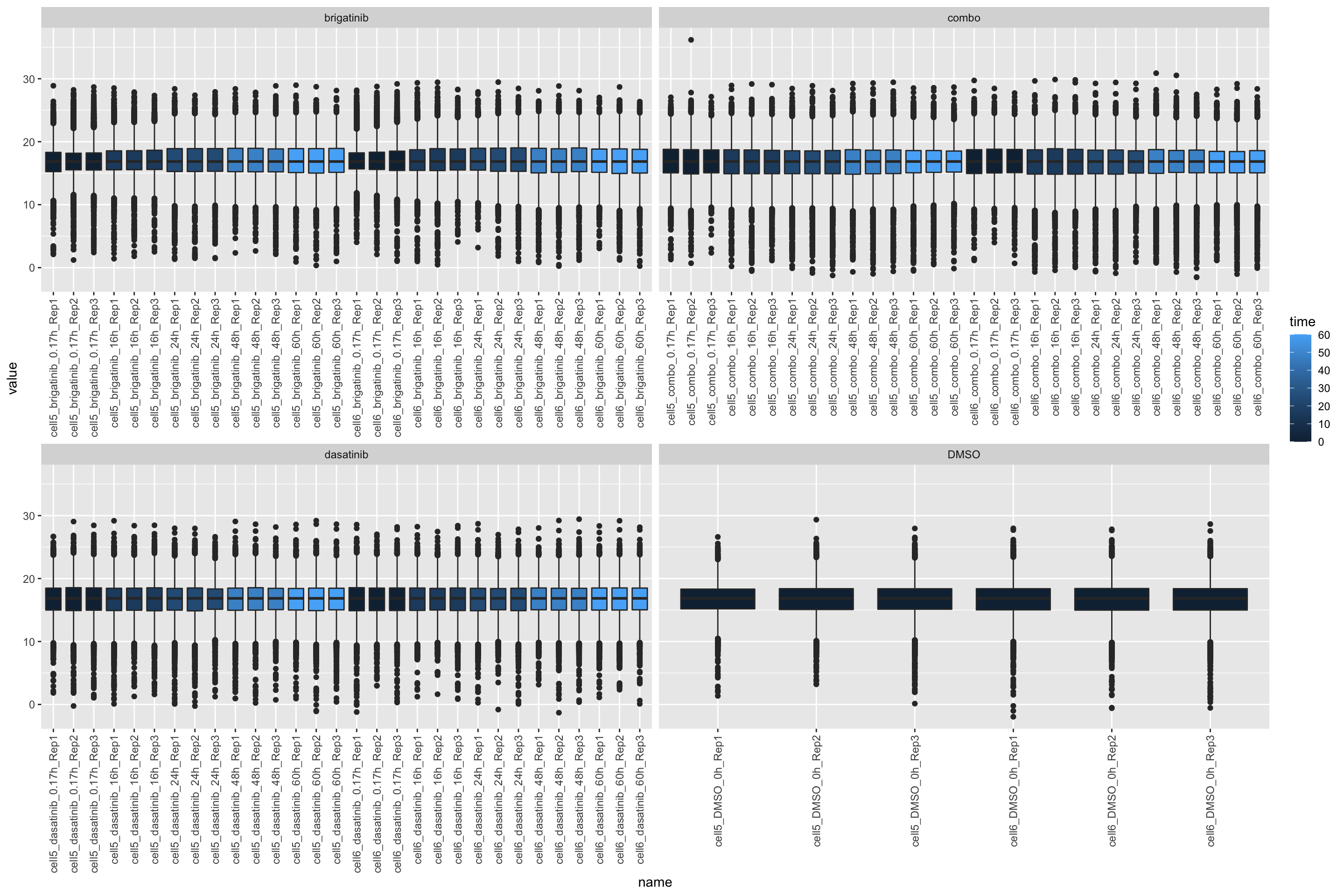

#### only transformation

countMat <- assay(ppe.log2Only)
annoTab <- colData(ppe.log2Only)[,c("sample","time","drug")] %>% as_tibble()
countTab <- countMat %>% as_tibble(rownames = "id") %>% 
    pivot_longer(-id) %>%
    filter(!is.na(value)) %>%
    left_join(annoTab, by = c(name = "sample"))
ggplot(countTab, aes(x=name, y=value)) +
    geom_boxplot(aes(fill = time)) +
    facet_wrap(~drug, scales = "free_x") +
    theme(axis.text.x = element_text(angle = 90, hjust = 1, vjust = 0.5))

use precursor

countMat <- assay(ppe.pre)
annoTab <- colData(ppe.pre)[,c("sample","time","drug")] %>% as_tibble()
countTab <- countMat %>% as_tibble(rownames = "id") %>% 
    pivot_longer(-id) %>%
    filter(!is.na(value)) %>%
    left_join(annoTab, by = c(name = "sample"))
ggplot(countTab, aes(x=name, y=value)) +
    geom_boxplot(aes(fill = time)) +
    facet_wrap(~drug, scales = "free_x") +
    theme(axis.text.x = element_text(angle = 90, hjust = 1, vjust = 0.5))

PCA

VST

exprMat <- assays(ppe.vst)[["imputed"]]
sds <- genefilter::rowSds(exprMat)
exprMat <- exprMat[order(sds, decreasing = TRUE)[1:2000],]

smpAnno <- colData(ppe.vst) %>%
    as_tibble(rownames = "id")

pcRes <- prcomp(t(exprMat), scale. = TRUE, center = TRUE)
pcTab <- pcRes$x[,1:10] %>% 
    as_tibble(rownames = "id") %>%
    left_join(smpAnno)

PC1 versus PC2

ggplot(pcTab, aes(x=PC1, y=PC2)) +
    geom_point(aes(col = drug, size = factor(time),
               shape = replicate)) +
    ggrepel::geom_text_repel(aes(label = id)) +
    theme_bw()

PC3 versus PC4

ggplot(pcTab, aes(x=PC3, y=PC4)) +
        geom_point(aes(col = drug, size = factor(time),
               shape = replicate)) +
    ggrepel::geom_text_repel(aes(label = id)) +
    theme_bw()

log2+median

exprMat <- assays(ppe.log2Med)[["imputed"]]
sds <- genefilter::rowSds(exprMat)
exprMat <- exprMat[order(sds, decreasing = TRUE)[1:2000],]

smpAnno <- colData(ppe.log2Med) %>%
    as_tibble(rownames = "id")

pcRes <- prcomp(t(exprMat), scale. = TRUE, center = TRUE)
pcTab <- pcRes$x[,1:10] %>% 
    as_tibble(rownames = "id") %>%
    left_join(smpAnno)

PC1 versus PC2

ggplot(pcTab, aes(x=PC1, y=PC2)) +
    geom_point(aes(col = drug, size = factor(time),
               shape = replicate)) +
    ggrepel::geom_text_repel(aes(label = id)) +
    theme_bw()

PC3 versus PC4

ggplot(pcTab, aes(x=PC3, y=PC4)) +
        geom_point(aes(col = drug, size = factor(time),
               shape = replicate)) +
    ggrepel::geom_text_repel(aes(label = id)) +
    theme_bw()

log2 only

exprMat <- assays(ppe.log2Only)[["imputed"]]
sds <- genefilter::rowSds(exprMat)
exprMat <- exprMat[order(sds, decreasing = TRUE)[1:2000],]

smpAnno <- colData(ppe.log2Only) %>%
    as_tibble(rownames = "id")

pcRes <- prcomp(t(exprMat), scale. = TRUE, center = TRUE)
pcTab <- pcRes$x[,1:10] %>% 
    as_tibble(rownames = "id") %>%
    left_join(smpAnno)

PC1 versus PC2

ggplot(pcTab, aes(x=PC1, y=PC2)) +
    geom_point(aes(col = drug, size = factor(time),
               shape = replicate)) +
    ggrepel::geom_text_repel(aes(label = id)) +
    theme_bw()

PC3 versus PC4

ggplot(pcTab, aes(x=PC3, y=PC4)) +
        geom_point(aes(col = drug, size = factor(time),
               shape = replicate)) +
    ggrepel::geom_text_repel(aes(label = id)) +
    theme_bw()

Use precursor

exprMat <- assays(ppe.pre)[["imputed"]]
sds <- genefilter::rowSds(exprMat)
exprMat <- exprMat[order(sds, decreasing = TRUE)[1:2000],]

smpAnno <- colData(ppe.pre) %>%
    as_tibble(rownames = "id")

pcRes <- prcomp(t(exprMat), scale. = TRUE, center = TRUE)
pcTab <- pcRes$x[,1:10] %>% 
    as_tibble(rownames = "id") %>%
    left_join(smpAnno)

PC1 versus PC2

ggplot(pcTab, aes(x=PC1, y=PC2)) +
    geom_point(aes(col = drug, size = factor(time),
               shape = replicate)) +
    ggrepel::geom_text_repel(aes(label = id)) +
    theme_bw()

PC3 versus PC4

ggplot(pcTab, aes(x=PC3, y=PC4)) +
        geom_point(aes(col = drug, size = factor(time),
               shape = replicate)) +
    ggrepel::geom_text_repel(aes(label = id)) +
    theme_bw()

Hierarchical clustering

VST

colAnno <- colData(ppe.vst)[,c("cellLine","drug","time")] %>% data.frame()
exprMat.scaled <- jyluMisc::mscale(exprMat, center = TRUE, scale = TRUE, censor = 5)
pheatmap::pheatmap(exprMat.scaled, annotation_col = colAnno, clustering_method = "ward.D2",
                   color = colorRampPalette(c("blue","white","red"))(100), 
                   breaks = seq(-5,5, length.out = 101), 
                   show_rownames = FALSE)

log2+median

colAnno <- colData(ppe.log2Med)[,c("cellLine","drug","time")] %>% data.frame()
exprMat.scaled <- jyluMisc::mscale(exprMat, center = TRUE, scale = TRUE, censor = 5)
pheatmap::pheatmap(exprMat.scaled, annotation_col = colAnno, clustering_method = "ward.D2",
                   color = colorRampPalette(c("blue","white","red"))(100), 
                   breaks = seq(-5,5, length.out = 101), 
                   show_rownames = FALSE)

log2 only

colAnno <- colData(ppe.log2Only)[,c("cellLine","drug","time")] %>% data.frame()
exprMat.scaled <- jyluMisc::mscale(exprMat, center = TRUE, scale = TRUE, censor = 5)
pheatmap::pheatmap(exprMat.scaled, annotation_col = colAnno, clustering_method = "ward.D2",
                   color = colorRampPalette(c("blue","white","red"))(100), 
                   breaks = seq(-5,5, length.out = 101), 
                   show_rownames = FALSE)

precursor

colAnno <- colData(ppe.pre)[,c("cellLine","drug","time")] %>% data.frame()
exprMat.scaled <- jyluMisc::mscale(exprMat, center = TRUE, scale = TRUE, censor = 5)
pheatmap::pheatmap(exprMat.scaled, annotation_col = colAnno, clustering_method = "ward.D2",
                   color = colorRampPalette(c("blue","white","red"))(100), 
                   breaks = seq(-5,5, length.out = 101), 
                   show_rownames = FALSE)

Compare the reproducibiliy of replicates when using different normalization methods

sdTab.vst <- getSdTab(ppe.vst) %>% mutate(norm = "vst")
sdTab.log2Med <- getSdTab(ppe.log2Med) %>% mutate(norm = "log2Med")
sdTab.log2Only <- getSdTab(ppe.log2Only) %>% mutate(norm = "log2Only")
sdTab.pre <- getSdTab(ppe.pre) %>% mutate(norm = "precursor")
sumTab <- bind_rows(sdTab.vst, sdTab.log2Med, sdTab.log2Only, sdTab.pre)

Add annotations

colTab <- colData(ppe.vst) %>% as_tibble() %>%
  distinct(sampleCondi,.keep_all = TRUE)
sumTab <- left_join(sumTab, colTab)

Overall distribution

ggplot(sumTab, aes(x=sdVal, fill = norm)) +
  geom_histogram(position = "identity", alpha=0.5, color = "grey50") +
  xlim(0,6)

Per sample

ggplot(sumTab, aes(x=sampleCondi, y = sdVal, fill = norm)) +
  geom_violin() +
  facet_wrap(~drug, scale="free_x")+
  theme(axis.text.x = element_text(angle = 90, hjust = 1, vjust = 0.5))

Mean versus SD

ggplot(sumTab, aes(x=meanVal, y=sdVal)) +
  geom_hex() + geom_smooth()  +
  facet_wrap(~norm, ncol=1)

Rank of sd for each normalization method

ordTab <- group_by(sumTab, sampleCondi, rowID) %>%
  mutate(index = order(sdVal))
ggplot(ordTab, aes(x=index, fill = norm)) +
  geom_bar(position = "dodge", alpha=0.5, color = "grey50")

For each sample, which normalization method gives the best reproduciblity for replicates

ordPerTab <- arrange(ordTab, index) %>% distinct(sampleCondi, drug,.keep_all = TRUE) %>%
  group_by(sampleCondi, norm, drug) %>% summarise(n=length(rowID))
ggplot(ordPerTab, aes(x=sampleCondi, y = n, fill = norm)) +
  geom_bar(stat="identity")+
  facet_wrap(~drug, scale = "free_x") +
  theme(axis.text.x = element_text(angle = 90, hjust = 1, vjust = 0.5))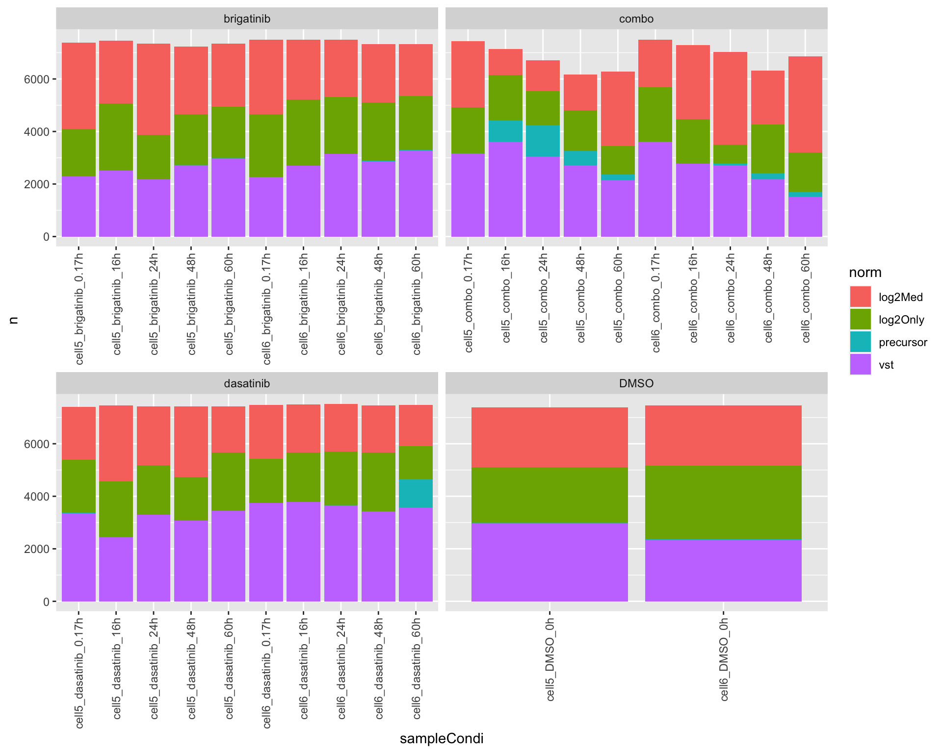

It seems log2 + median scaling can get the best reproducibility among replicates. No normalization is the worst.

Phosphoproteomic with proteomic regressed out

Preprocessing

ppeSub <- preprocessPhos(maeData, normalize = TRUE, transform = "none", assayName = "PhosReg")

[1] "Number of proteins and samples:"
[1] 3574   96

Distribution after normalization

countMat <- assay(ppeSub)
annoTab <- colData(ppeSub)[,c("sample","time","drug")] %>% as_tibble()
countTab <- countMat %>% as_tibble(rownames = "id") %>% 
    pivot_longer(-id) %>%
    filter(!is.na(value)) %>%
    left_join(annoTab, by = c(name = "sample"))

ggplot(countTab, aes(x=name, y=value)) +
    geom_boxplot(aes(fill = time)) +
    facet_wrap(~drug, scales = "free_x") +
    theme(axis.text.x = element_text(angle = 90, hjust = 1, vjust = 0.5))

PCA

exprMat <- assays(ppeSub)[["imputed"]]
sds <- genefilter::rowSds(exprMat)
exprMat <- exprMat[order(sds, decreasing = TRUE)[1:1000],]

smpAnno <- colData(ppeSub) %>%
    as_tibble(rownames = "id")

pcRes <- prcomp(t(exprMat), scale. = TRUE, center = TRUE)
pcTab <- pcRes$x[,1:10] %>% 
    as_tibble(rownames = "id") %>%
    left_join(smpAnno)

PC1 versus PC2

ggplot(pcTab, aes(x=PC1, y=PC2)) +
    geom_point(aes(col = drug, size = factor(time),
               shape = replicate)) +
    ggrepel::geom_text_repel(aes(label = id)) +
    theme_bw()

PC3 versus PC4

ggplot(pcTab, aes(x=PC3, y=PC4)) +
        geom_point(aes(col = drug, size = factor(time),
               shape = replicate)) +
    ggrepel::geom_text_repel(aes(label = id)) +
    theme_bw()

Hierarchical clustering

colAnno <- colData(ppeSub)[,c("cellLine","drug","time")] %>% data.frame()
exprMat.scaled <- jyluMisc::mscale(exprMat, center = TRUE, scale = TRUE, censor = 5)
pheatmap::pheatmap(exprMat.scaled, annotation_col = colAnno, clustering_method = "ward.D2",
                   color = colorRampPalette(c("blue","white","red"))(100), 
                   breaks = seq(-5,5, length.out = 101), 
                   show_rownames = FALSE)

Remove one potential outlier

ppeSub <- ppeSub[, colnames(ppeSub)!="cell5_combo_24h_Rep2"]

Redo PCA

exprMat <- assays(ppeSub)[["imputed"]]
sds <- genefilter::rowSds(exprMat)
exprMat <- exprMat[order(sds, decreasing = TRUE)[1:1000],]

smpAnno <- colData(ppeSub) %>%
    as_tibble(rownames = "id")

pcRes <- prcomp(t(exprMat), scale. = TRUE, center = TRUE)
pcTab <- pcRes$x[,1:10] %>% 
    as_tibble(rownames = "id") %>%
    left_join(smpAnno)

PC1 versus PC2

ggplot(pcTab, aes(x=PC1, y=PC2)) +
    geom_point(aes(col = drug, size = factor(time),
               shape = replicate)) +
    ggrepel::geom_text_repel(aes(label = id)) +
    theme_bw()

PC3 versus PC4

ggplot(pcTab, aes(x=PC3, y=PC4)) +
        geom_point(aes(col = drug, size = factor(time),
               shape = replicate)) +
    ggrepel::geom_text_repel(aes(label = id)) +
    theme_bw()

Hierarchical clustering

colAnno <- colData(ppeSub)[,c("cellLine","drug","time")] %>% data.frame()
exprMat.scaled <- jyluMisc::mscale(exprMat, center = TRUE, scale = TRUE, censor = 5)
pheatmap::pheatmap(exprMat.scaled, annotation_col = colAnno, clustering_method = "ward.D2",
                   color = colorRampPalette(c("blue","white","red"))(100), 
                   breaks = seq(-5,5, length.out = 101), 
                   show_rownames = FALSE)

Use ration between phosphoproteome and proteome

Preprocessing

ppeSub <- preprocessPhos(maeData, normalize = TRUE, transform = "none", assayName = "PhosRatio")

[1] "Number of proteins and samples:"
[1] 3574   96

Distribution after normalization

countMat <- assay(ppeSub)
annoTab <- colData(ppeSub)[,c("sample","time","drug")] %>% as_tibble()
countTab <- countMat %>% as_tibble(rownames = "id") %>% 
    pivot_longer(-id) %>%
    filter(!is.na(value)) %>%
    left_join(annoTab, by = c(name = "sample"))

ggplot(countTab, aes(x=name, y=value)) +
    geom_boxplot(aes(fill = time)) +
    facet_wrap(~drug, scales = "free_x") +
    theme(axis.text.x = element_text(angle = 90, hjust = 1, vjust = 0.5))

PCA

exprMat <- assays(ppeSub)[["imputed"]]
sds <- genefilter::rowSds(exprMat)
exprMat <- exprMat[order(sds, decreasing = TRUE)[1:1000],]

smpAnno <- colData(ppeSub) %>%
    as_tibble(rownames = "id")

pcRes <- prcomp(t(exprMat), scale. = TRUE, center = TRUE)
pcTab <- pcRes$x[,1:10] %>% 
    as_tibble(rownames = "id") %>%
    left_join(smpAnno)

PC1 versus PC2

ggplot(pcTab, aes(x=PC1, y=PC2)) +
    geom_point(aes(col = drug, size = factor(time),
               shape = replicate)) +
    ggrepel::geom_text_repel(aes(label = id)) +
    theme_bw()

PC3 versus PC4

ggplot(pcTab, aes(x=PC3, y=PC4)) +
        geom_point(aes(col = drug, size = factor(time),
               shape = replicate)) +
    ggrepel::geom_text_repel(aes(label = id)) +
    theme_bw()

Hierarchical clustering

colAnno <- colData(ppeSub)[,c("cellLine","drug","time")] %>% data.frame()
exprMat.scaled <- jyluMisc::mscale(exprMat, center = TRUE, scale = TRUE, censor = 5)
pheatmap::pheatmap(exprMat.scaled, annotation_col = colAnno, clustering_method = "ward.D2",
                   color = colorRampPalette(c("blue","white","red"))(100), 
                   breaks = seq(-5,5, length.out = 101), 
                   show_rownames = FALSE)

Remove one potential outlier

ppeSub <- ppeSub[, colnames(ppeSub)!="cell5_combo_24h_Rep2"]

Redo PCA

exprMat <- assays(ppeSub)[["imputed"]]
sds <- genefilter::rowSds(exprMat)
exprMat <- exprMat[order(sds, decreasing = TRUE)[1:1000],]

smpAnno <- colData(ppeSub) %>%
    as_tibble(rownames = "id")

pcRes <- prcomp(t(exprMat), scale. = TRUE, center = TRUE)
pcTab <- pcRes$x[,1:10] %>% 
    as_tibble(rownames = "id") %>%
    left_join(smpAnno)

PC1 versus PC2

ggplot(pcTab, aes(x=PC1, y=PC2)) +
    geom_point(aes(col = drug, size = factor(time),
               shape = replicate)) +
    ggrepel::geom_text_repel(aes(label = id)) +
    theme_bw()

PC3 versus PC4

ggplot(pcTab, aes(x=PC3, y=PC4)) +
        geom_point(aes(col = drug, size = factor(time),
               shape = replicate)) +
    ggrepel::geom_text_repel(aes(label = id)) +
    theme_bw()

Hierarchical clustering

colAnno <- colData(ppeSub)[,c("cellLine","drug","time")] %>% data.frame()
exprMat.scaled <- jyluMisc::mscale(exprMat, center = TRUE, scale = TRUE, censor = 5)
pheatmap::pheatmap(exprMat.scaled, annotation_col = colAnno, clustering_method = "ward.D2",
                   color = colorRampPalette(c("blue","white","red"))(100), 
                   breaks = seq(-5,5, length.out = 101), 
                   show_rownames = FALSE)

sessionInfo()

R version 4.2.0 (2022-04-22)
Platform: x86_64-apple-darwin17.0 (64-bit)
Running under: macOS Big Sur/Monterey 10.16

Matrix products: default
BLAS:   /Library/Frameworks/R.framework/Versions/4.2/Resources/lib/libRblas.0.dylib
LAPACK: /Library/Frameworks/R.framework/Versions/4.2/Resources/lib/libRlapack.dylib

locale:
[1] en_US.UTF-8/en_US.UTF-8/en_US.UTF-8/C/en_US.UTF-8/en_US.UTF-8

attached base packages:
[1] stats4    stats     graphics  grDevices utils     datasets  methods  
[8] base     

other attached packages:
 [1] forcats_0.5.1               stringr_1.4.1              
 [3] dplyr_1.0.9                 purrr_0.3.4                
 [5] readr_2.1.2                 tidyr_1.2.0                
 [7] tibble_3.1.8                ggplot2_3.3.6              
 [9] tidyverse_1.3.2             proDA_1.10.0               
[11] MultiAssayExperiment_1.22.0 SummarizedExperiment_1.26.1
[13] Biobase_2.56.0              GenomicRanges_1.48.0       
[15] GenomeInfoDb_1.32.2         IRanges_2.30.0             
[17] S4Vectors_0.34.0            BiocGenerics_0.42.0        
[19] MatrixGenerics_1.8.1        matrixStats_0.62.0         

loaded via a namespace (and not attached):
  [1] GGally_2.1.2           exactRankTests_0.8-35  coda_0.19-4           
  [4] bit64_4.0.5            knitr_1.39             multcomp_1.4-19       
  [7] DelayedArray_0.22.0    data.table_1.14.2      KEGGREST_1.36.3       
 [10] RCurl_1.98-1.7         doParallel_1.0.17      generics_0.1.3        
 [13] preprocessCore_1.58.0  cowplot_1.1.1          TH.data_1.1-1         
 [16] RSQLite_2.2.15         proxy_0.4-27           bit_4.0.4             
 [19] tzdb_0.3.0             xml2_1.3.3             lubridate_1.8.0       
 [22] httpuv_1.6.6           assertthat_0.2.1       viridis_0.6.2         
 [25] gargle_1.2.0           xfun_0.31              hms_1.1.1             
 [28] jquerylib_0.1.4        evaluate_0.15          promises_1.2.0.1      
 [31] fansi_1.0.3            caTools_1.18.2         dendextend_1.16.0     
 [34] dbplyr_2.2.1           readxl_1.4.0           km.ci_0.5-6           
 [37] igraph_1.3.4           DBI_1.1.3              htmlwidgets_1.5.4     
 [40] reshape_0.8.9          googledrive_2.0.0      ellipsis_0.3.2        
 [43] jyluMisc_0.1.5         ggpubr_0.4.0           backports_1.4.1       
 [46] annotate_1.74.0        PhosR_1.6.0            vctrs_0.4.1           
 [49] imputeLCMD_2.1         abind_1.4-5            cachem_1.0.6          
 [52] withr_2.5.0            cluster_2.1.3          crayon_1.5.2          
 [55] drc_3.0-1              relations_0.6-12       genefilter_1.78.0     
 [58] pkgconfig_2.0.3        slam_0.1-50            labeling_0.4.2        
 [61] nlme_3.1-158           ProtGenerics_1.28.0    rlang_1.0.6           
 [64] lifecycle_1.0.3        sandwich_3.0-2         affyio_1.66.0         
 [67] modelr_0.1.8           cellranger_1.1.0       rprojroot_2.0.3       
 [70] Matrix_1.4-1           KMsurv_0.1-5           carData_3.0-5         
 [73] zoo_1.8-10             DEP_1.18.0             reprex_2.0.1          
 [76] GlobalOptions_0.1.2    googlesheets4_1.0.0    pheatmap_1.0.12       
 [79] png_0.1-7              viridisLite_0.4.0      rjson_0.2.21          
 [82] mzR_2.30.0             bitops_1.0-7           shinydashboard_0.7.2  
 [85] visNetwork_2.1.0       KernSmooth_2.23-20     Biostrings_2.64.0     
 [88] blob_1.2.3             workflowr_1.7.0        shape_1.4.6           
 [91] maxstat_0.7-25         rstatix_0.7.0          tmvtnorm_1.5          
 [94] ggsignif_0.6.3         scales_1.2.0           memoise_2.0.1         
 [97] magrittr_2.0.3         plyr_1.8.7             hexbin_1.28.2         
[100] gplots_3.1.3           zlibbioc_1.42.0        compiler_4.2.0        
[103] RColorBrewer_1.1-3     plotrix_3.8-2          pcaMethods_1.88.0     
[106] clue_0.3-61            cli_3.4.1              affy_1.74.0           
[109] XVector_0.36.0         mgcv_1.8-40            MASS_7.3-58           
[112] tidyselect_1.1.2       vsn_3.64.0             stringi_1.7.8         
[115] highr_0.9              yaml_2.3.5             norm_1.0-10.0         
[118] MALDIquant_1.21        ggrepel_0.9.1          survMisc_0.5.6        
[121] grid_4.2.0             sass_0.4.2             fastmatch_1.1-3       
[124] tools_4.2.0            ruv_0.9.7.1            parallel_4.2.0        
[127] circlize_0.4.15        rstudioapi_0.13        MsCoreUtils_1.8.0     
[130] foreach_1.5.2          git2r_0.30.1           gridExtra_2.3         
[133] farver_2.1.1           mzID_1.34.0            digest_0.6.30         
[136] BiocManager_1.30.18    shiny_1.7.3            Rcpp_1.0.9            
[139] car_3.1-0              broom_1.0.0            later_1.3.0           
[142] ncdf4_1.19             survminer_0.4.9        httr_1.4.3            
[145] MSnbase_2.22.0         ggdendro_0.1.23        AnnotationDbi_1.58.0  
[148] ComplexHeatmap_2.12.0  colorspace_2.0-3       rvest_1.0.2           
[151] XML_3.99-0.10          fs_1.5.2               splines_4.2.0         
[154] gmm_1.6-6              xtable_1.8-4           jsonlite_1.8.3        
[157] marray_1.74.0          R6_2.5.1               sets_1.0-21           
[160] pillar_1.8.0           htmltools_0.5.3        mime_0.12             
[163] glue_1.6.2             fastmap_1.1.0          DT_0.23               
[166] BiocParallel_1.30.3    class_7.3-20           codetools_0.2-18      
[169] fgsea_1.22.0           mvtnorm_1.1-3          utf8_1.2.2            
[172] lattice_0.20-45        bslib_0.4.1            network_1.17.2        
[175] gtools_3.9.3           shinyjs_2.1.0          survival_3.4-0        
[178] limma_3.52.2           rmarkdown_2.14         statnet.common_4.6.0  
[181] munsell_0.5.0          e1071_1.7-11           GetoptLong_1.0.5      
[184] GenomeInfoDbData_1.2.8 iterators_1.0.14       piano_2.12.0          
[187] impute_1.70.0          haven_2.5.0            reshape2_1.4.4        
[190] gtable_0.3.0

Exploratory data analysis and QA

Load packages and dataset

Phosphoproteomic

Preprocessing

Mean SD plots

VST

Log2+median

log2 only

Distribution after normalization

VST

log2+median

use precursor

PCA

VST

log2+median

log2 only

Use precursor

Hierarchical clustering

VST

log2+median

log2 only

precursor

Remove one potential outlier

PCA

VST

log2+median

log2 only

Use precursor

Hierarchical clustering

VST

log2+median

log2 only

precursor

Compare the reproducibiliy of replicates when using different normalization methods

Proteomic

Preprocessing

Mean SD plots

VST

Log2+median

log2 only

Distribution after normalization

VST

log2+median

use precursor

PCA

VST

log2+median

log2 only

Use precursor

Hierarchical clustering

VST

log2+median

log2 only

precursor

Compare the reproducibiliy of replicates when using different normalization methods

Phosphoproteomic with proteomic regressed out

Preprocessing

Distribution after normalization

PCA

Hierarchical clustering

Remove one potential outlier

Redo PCA

Hierarchical clustering

Use ration between phosphoproteome and proteome

Preprocessing

Distribution after normalization

PCA

Hierarchical clustering

Remove one potential outlier

Redo PCA

Hierarchical clustering