Differential expression analysis on protein level (RUN5, no normalization by Spectronaut, vst normalization in R)
Last updated: 2023-02-14
Checks: 4 2
Knit directory:
LungCancer_SotilloLab/analysis/
This reproducible R Markdown analysis was created with workflowr (version 1.7.0). The Checks tab describes the reproducibility checks that were applied when the results were created. The Past versions tab lists the development history.
Great job! The global environment was empty. Objects defined in the global environment can affect the analysis in your R Markdown file in unknown ways. For reproduciblity it’s best to always run the code in an empty environment.
The command set.seed(20221103) was run prior to running
the code in the R Markdown file. Setting a seed ensures that any results
that rely on randomness, e.g. subsampling or permutations, are
reproducible.
Great job! Recording the operating system, R version, and package versions is critical for reproducibility.
- unnamed-chunk-19
- unnamed-chunk-23
- unnamed-chunk-32
- unnamed-chunk-36
- unnamed-chunk-64
- unnamed-chunk-74
- unnamed-chunk-78
To ensure reproducibility of the results, delete the cache directory
Focused_analysis_RUN5_vst_ProteinOnly_cache and re-run the
analysis. To have workflowr automatically delete the cache directory
prior to building the file, set delete_cache = TRUE when
running wflow_build() or wflow_publish().
Great job! Using relative paths to the files within your workflowr project makes it easier to run your code on other machines.
Tracking code development and connecting the code version to the
results is critical for reproducibility. To start using Git, open the
Terminal and type git init in your project directory.
This project is not being versioned with Git. To obtain the full
reproducibility benefits of using workflowr, please see
?wflow_start.
Load packages and dataset
Packages
#package
library(SummarizedExperiment)
library(MultiAssayExperiment)
library(proDA)
library(UpSetR)
library(tidyverse)
source("../code/utils.R")
knitr::opts_chunk$set(warning = FALSE, message = FALSE, autodep = TRUE)Pre-processed data
load("../output/processedData_RUN5.RData")
#load saved result list
load("../output/allResList_RUN5_timeBased.RData")
#List of mitochondiral genes
mitoList <- readxl::read_xls("../data/Mouse.MitoCarta3.0.xls", sheet = 2)$Symbol
#geneset files
gmts <- list(Hallmark = "../data/gmts/mh.all.v2022.1.Mm.symbols.gmt",
CanonicalPathway = "../data/gmts/m2.cp.v2022.1.Mm.symbols.gmt")Differential expression at 10 min (0.17 hour) for each drug
Preprocessing
filterList <- list(time = c(0.17,0))
fpeSub <- preprocessProteome(maeData, filterList, missCut = 0.5, transform = "vst", normalize = TRUE)[1] "Number of proteins and samples:"
[1] 7740 24Plot value distribution
plotTab <- jyluMisc::sumToTidy(fpeSub)
ggplot(plotTab, aes(x=sample, y=Intensity)) +
geom_boxplot(aes(fill = drug)) +
theme(axis.text.x = element_text(angle = 90, hjust = 1, vjust = 0.5))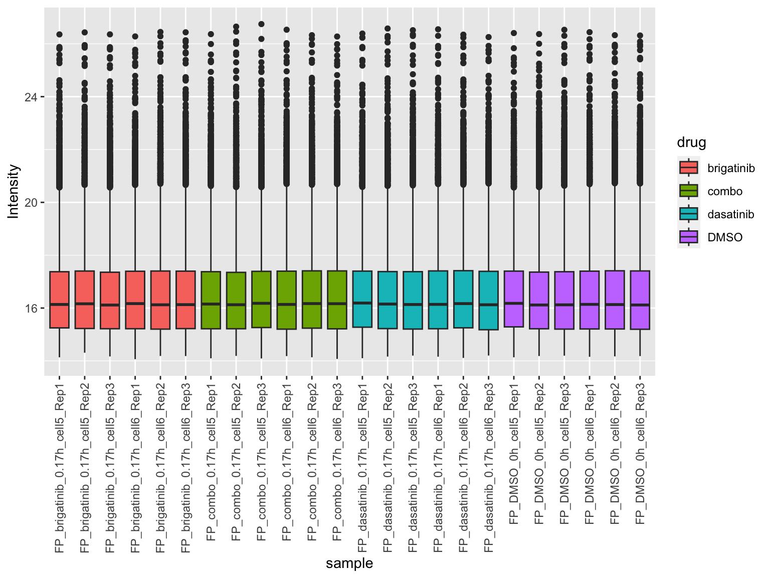
Expression of mitocondrial proteins
plotMitoTab <- filter(plotTab, Gene %in% mitoList)
ggplot(plotMitoTab, aes(x=sample, y=Intensity)) +
geom_boxplot(aes(fill = drug)) +
theme(axis.text.x = element_text(angle = 90, hjust = 1, vjust = 0.5))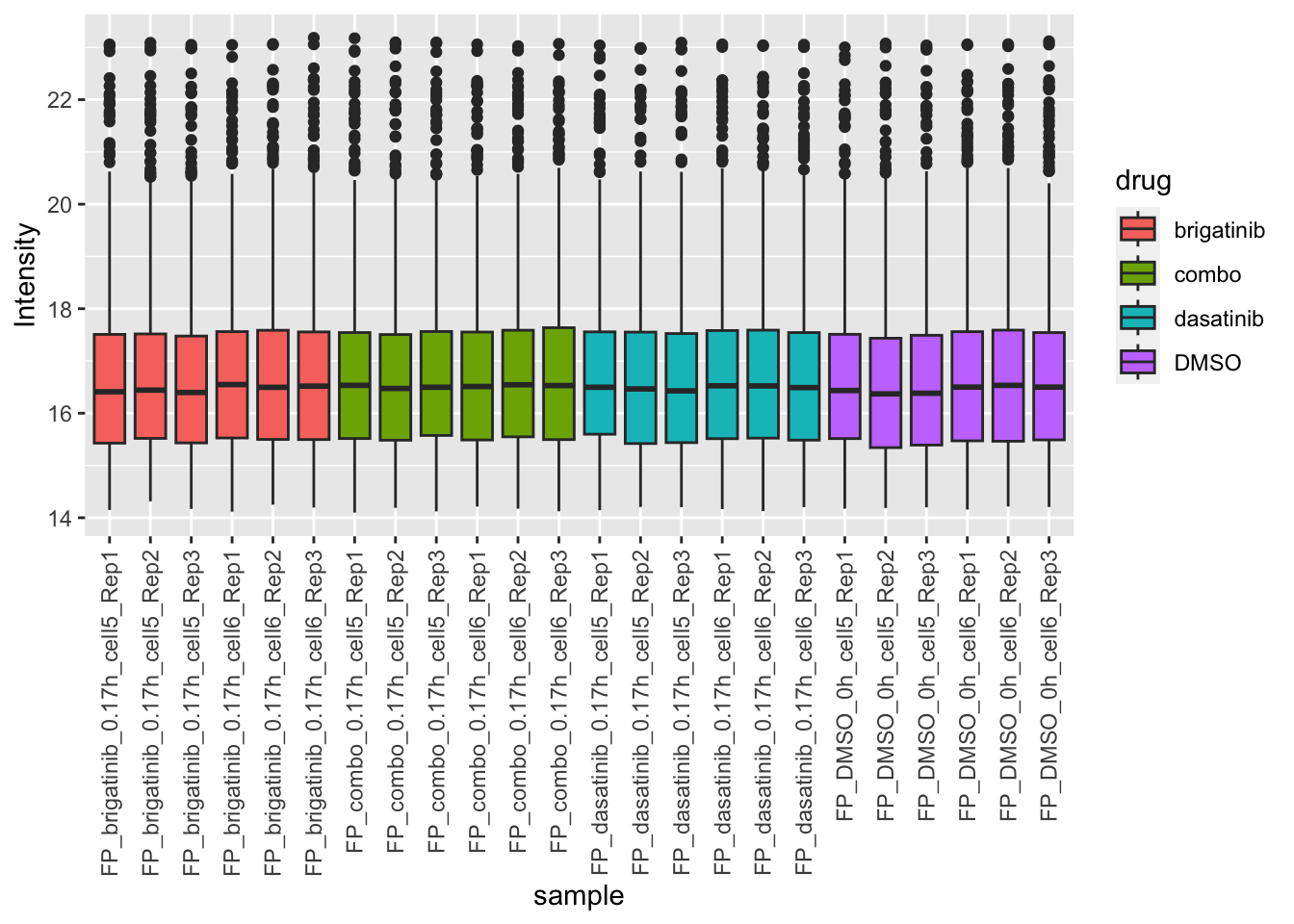 No strong difference
PCA
PC1 versus PC2
plotPCA(fpeSub, assayName = "imputed", "PC1", "PC2", topVar = 5000, label ="replicate")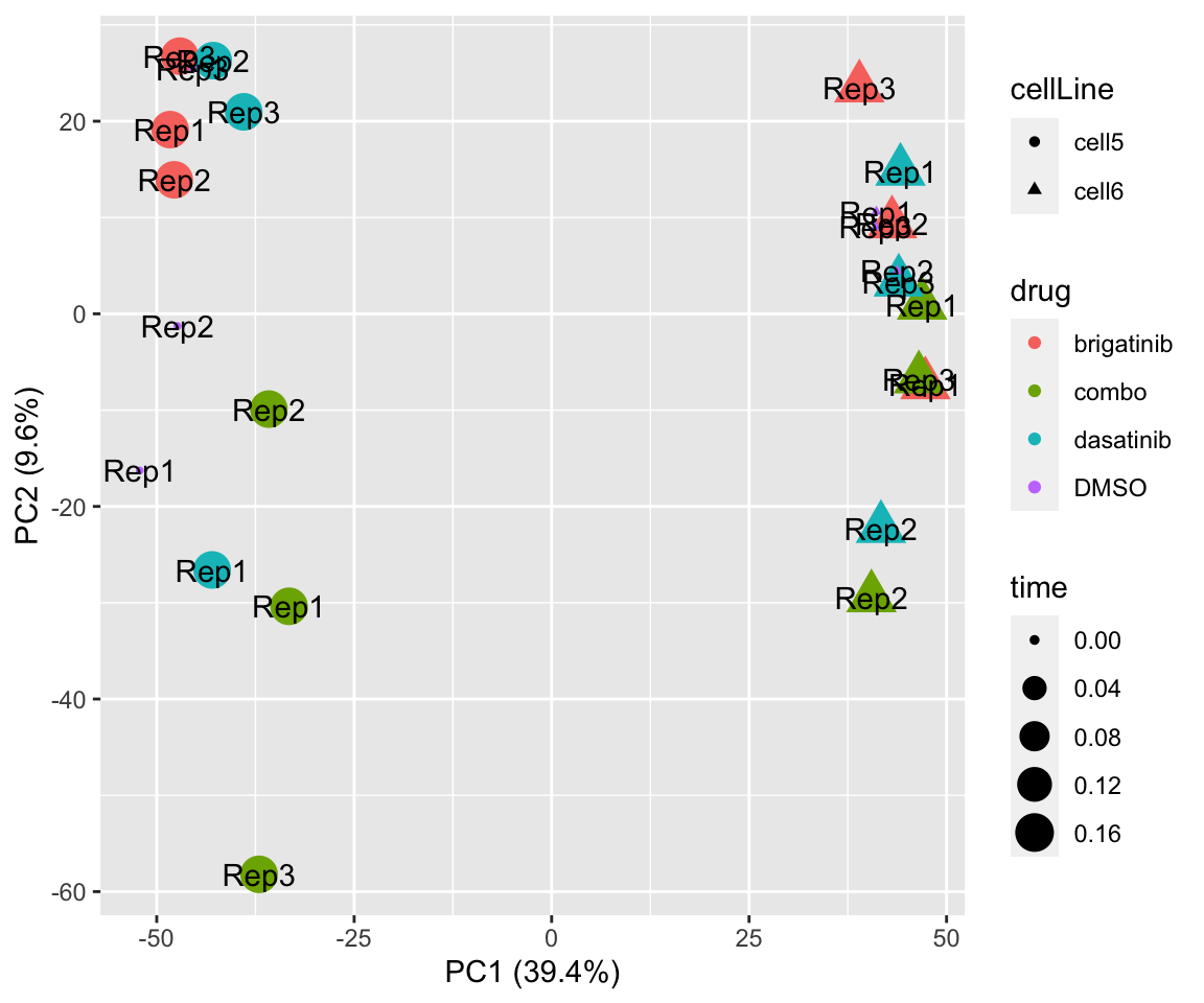
PC3 versus PC4
plotPCA(fpeSub, assayName = "imputed", "PC3", "PC4", topVar = 5000, label = "replicate")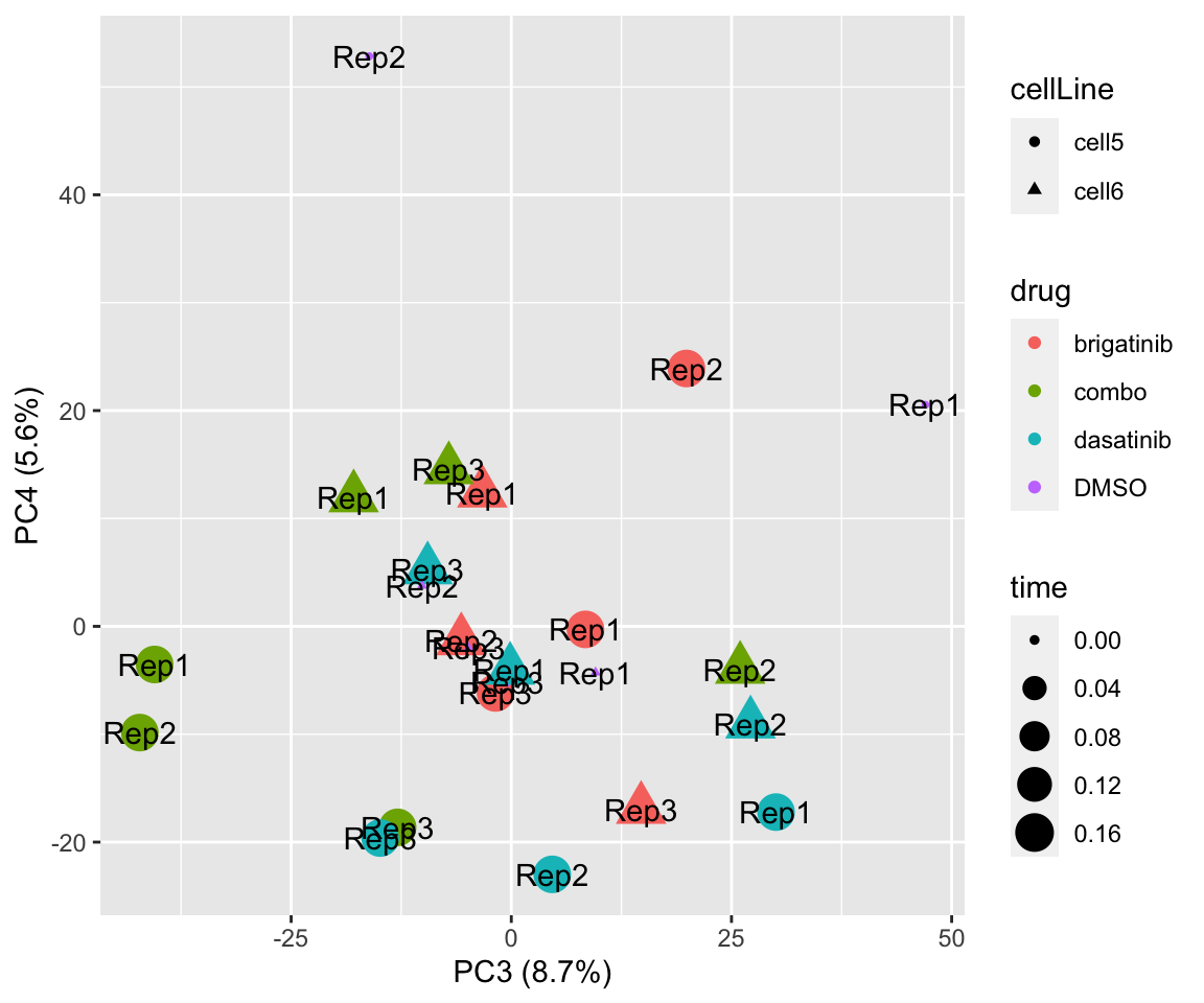
Differential expression using proDA
Load saved results
resTab <- allResList$diffProt$time_0.17 %>% filter(compare !="interaction")Table of significant associations (10% FDR)
resTab.sig <- filter(resTab, adj_pval <= 0.1)
resTab.sig %>% mutate(across(where(is.numeric), formatC, digits=2)) %>% DT::datatable()P-value histogram for each comparison
ggplot(resTab, aes(x=pval)) +
geom_histogram(bins = 20, fill = "lightblue", color = "grey50") +
facet_wrap(~compare)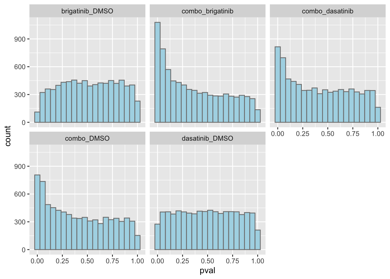
Number of DE proteins for each comparison (10% FDR)
sumTab <- filter(resTab, adj_pval < 0.1) %>%
mutate(direction = ifelse(diff>0, "Up","Down")) %>%
group_by(compare, direction) %>%
summarise(n=length(name))
ggplot(sumTab, aes(x=compare, y=n)) +
geom_bar(aes(fill = direction), stat = "identity", position = "dodge") +
coord_flip() +
geom_text(aes(label =n)) +
facet_wrap(~direction, ncol=2, scales = "free_x") +
xlab("Number")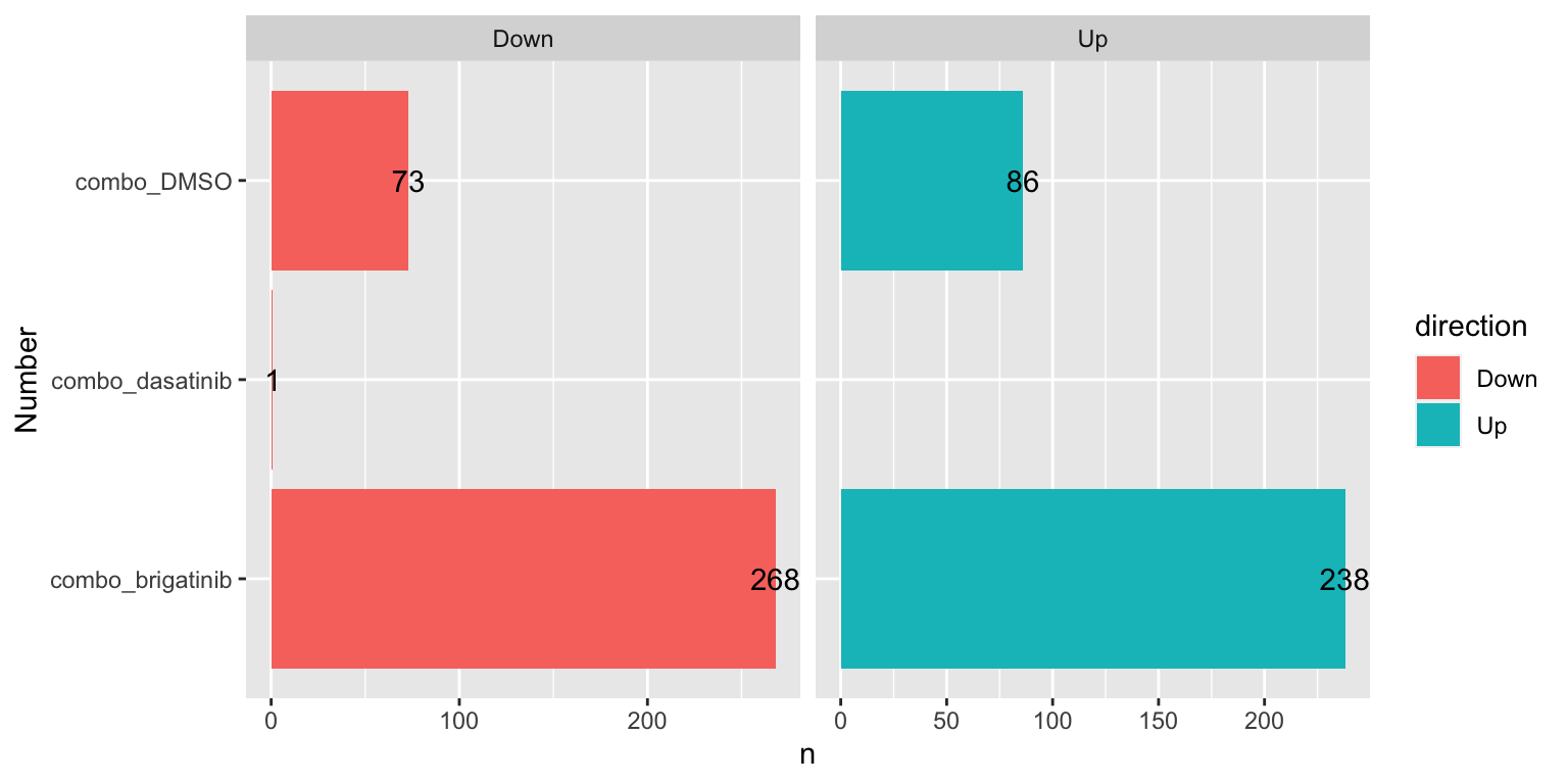
Number of DE mitochondrial proteins for each comparison (10% FDR)
sumTab <- filter(resTab, adj_pval < 0.1, symbol %in% mitoList) %>%
mutate(direction = ifelse(diff>0, "Up","Down")) %>%
group_by(compare, direction) %>%
summarise(n=length(name))
ggplot(sumTab, aes(x=compare, y=n)) +
geom_bar(aes(fill = direction), stat = "identity", position = "dodge") +
coord_flip() +
geom_text(aes(label =n)) +
facet_wrap(~direction, ncol=2, scales = "free_x") +
xlab("Number")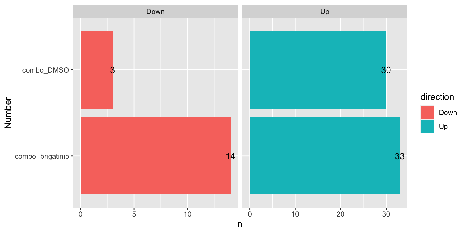
Heatmap of DE proteins for each treatment
Brigatinib versus DMSO
plotProteinHeatmap(resTab, fpeSub, "brigatinib_DMSO", fdrCut = 0.1, ifFDR = TRUE)[1] "Nothing to plot"Dasatinib versus DMSO
plotProteinHeatmap(resTab, fpeSub, "dasatinib_DMSO", fdrCut = 0.1, ifFDR =TRUE)[1] "Nothing to plot"Combo versus DMSO
plotProteinHeatmap(resTab, fpeSub, "combo_DMSO", fdrCut = 0.1, ifFDR = TRUE)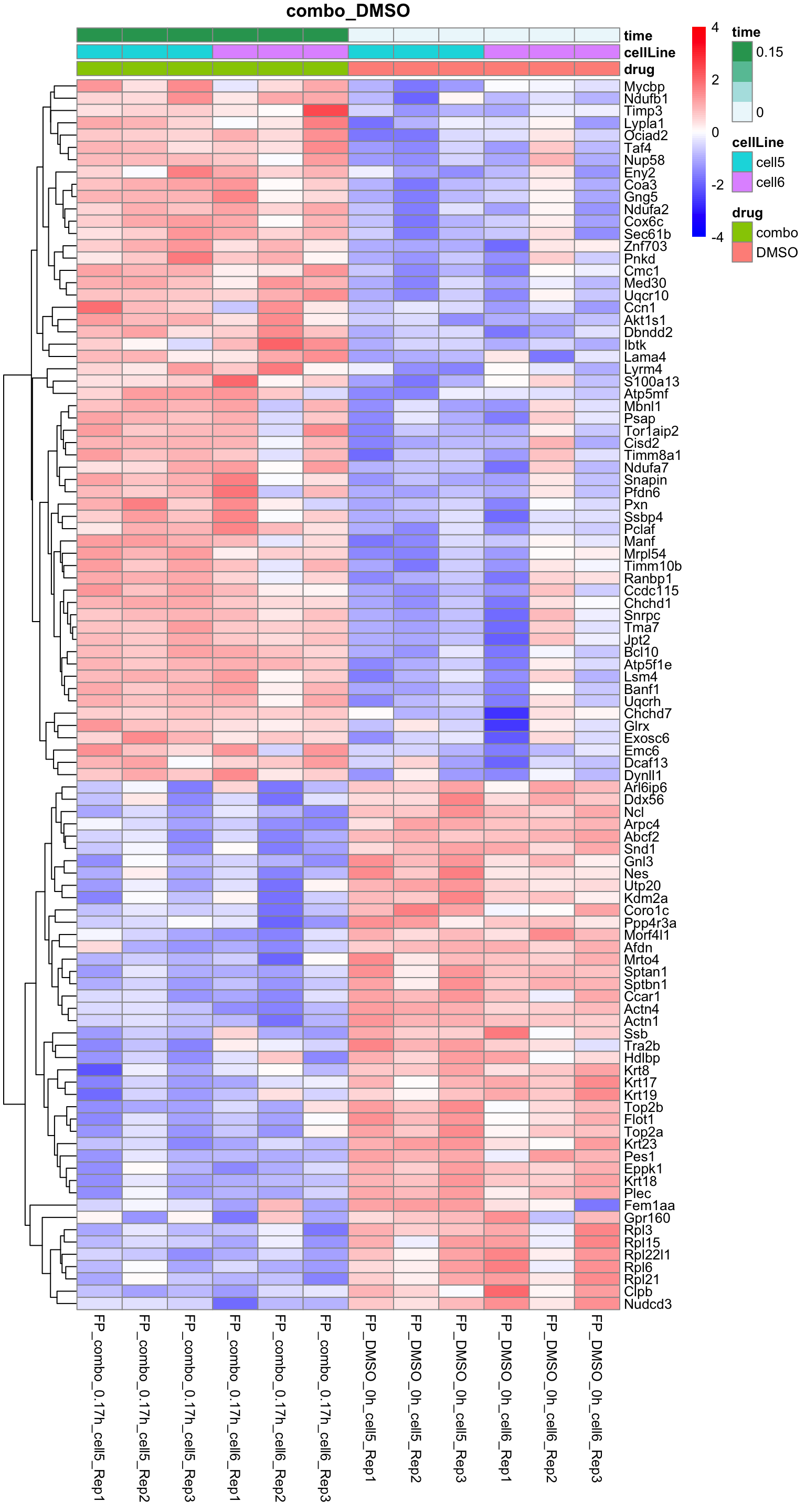
Combo versus brigatinib
plotProteinHeatmap(resTab, fpeSub, "combo_brigatinib", fdrCut = 0.1, ifFDR = TRUE)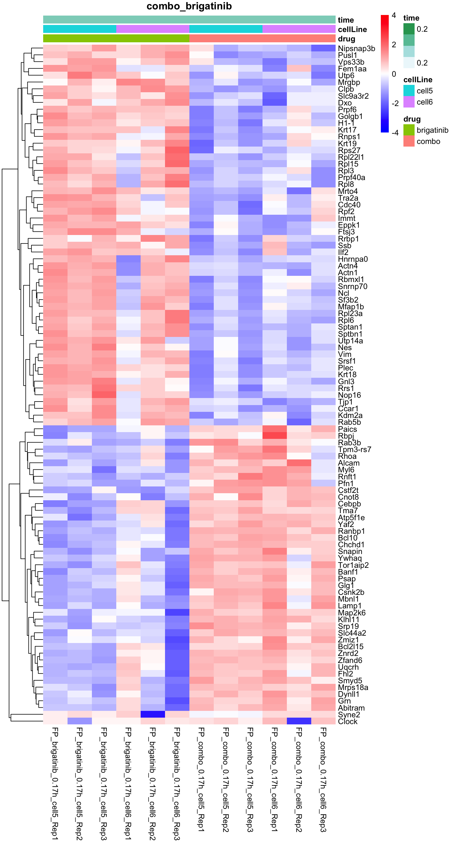
Combo versus dasatinib
plotProteinHeatmap(resTab, fpeSub, "combo_dasatinib", fdrCut = 0.1, ifFDR = TRUE)[1] "Nothing to plot"Overlap of DE proteins
Up regulated
deList <- lapply(unique(resTab$compare), function(x) {
filter(resTab, compare == x,adj_pval<0.1, diff >0)$name
})
names(deList) <- unique(resTab$compare)
upset(fromList(deList))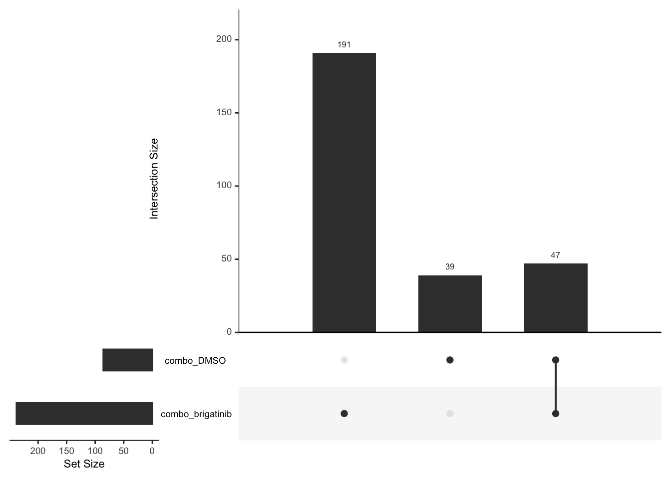
Down regulated
deList <- lapply(unique(resTab$compare), function(x) {
filter(resTab, compare == x, adj_pval <= 0.1, diff <0)$name
})
names(deList) <- unique(resTab$compare)
upset(fromList(deList))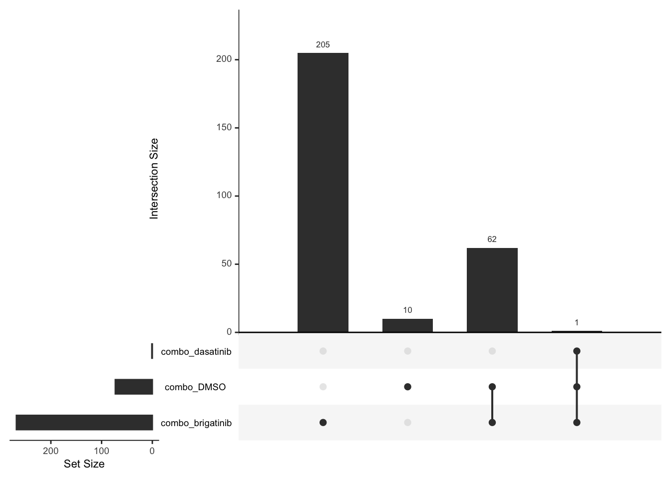
Gene set enrichment analysis
Define useful genesets
plotList <- runGeneSetEnrichment(resTab, gmts, genePCut = 1, pCutSet = 0.1, setFdr = TRUE, method="gsea", collapsePathway = TRUE)[1] "Testing for: Hallmark"
[1] "Condition: dasatinib_DMSO"
[1] "Condition: brigatinib_DMSO"
[1] "Condition: combo_DMSO"
[1] "Condition: combo_brigatinib"
[1] "Condition: combo_dasatinib"
[1] "Testing for: CanonicalPathway"
[1] "Condition: dasatinib_DMSO"
[1] "Condition: brigatinib_DMSO"
[1] "Condition: combo_DMSO"
[1] "Condition: combo_brigatinib"
[1] "Condition: combo_dasatinib"Hallmarks
plotList$Hallmark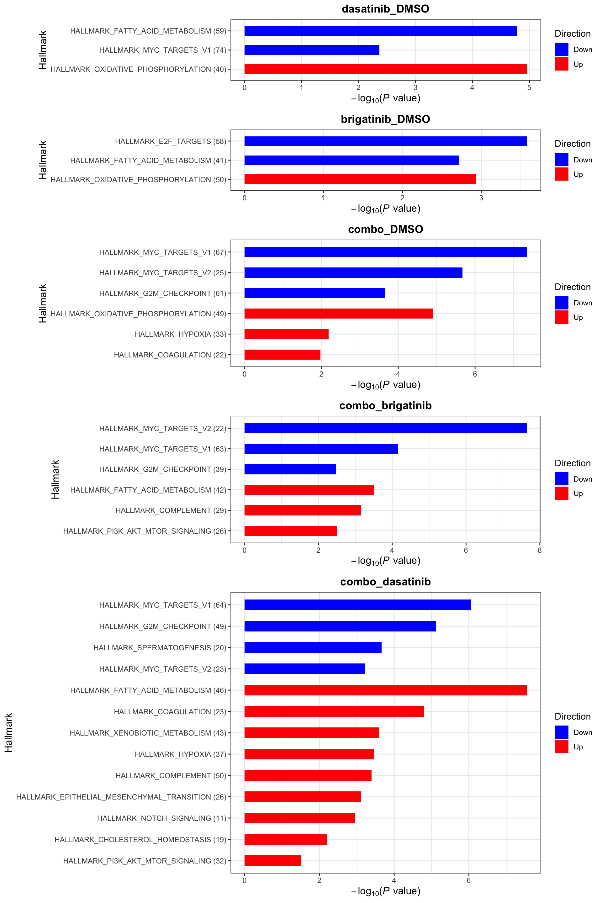
Canonical pathways
plotList$CanonicalPathway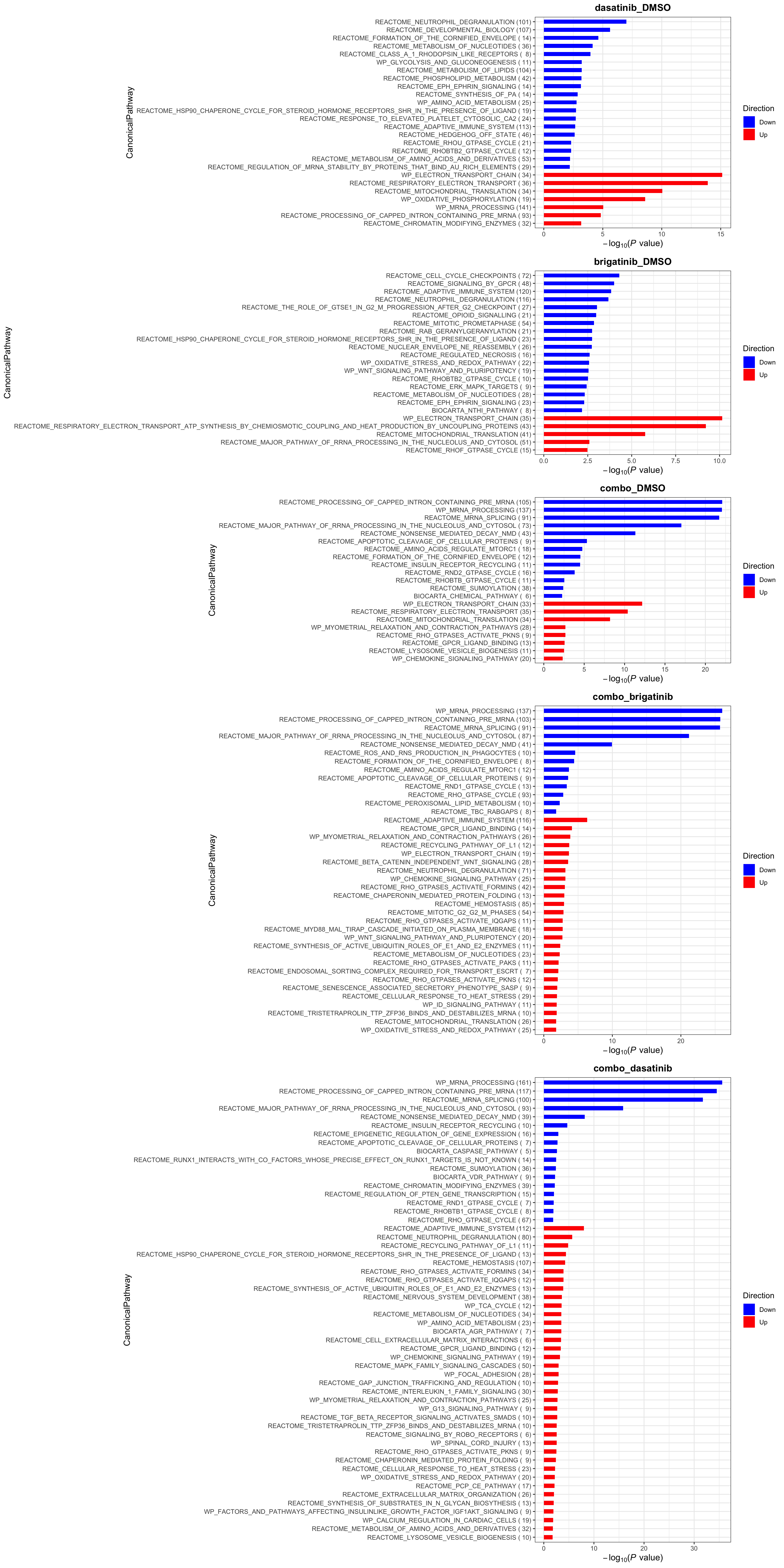
List of leading edge genes for each pathway
Leading edges genes are not necessarily significantly differentially expressed, but they contribute most to the enrichment analysis. Please see explaination of leading edge genes on this page: https://www.gsea-msigdb.org/gsea/doc/GSEAUserGuideFrame.html
DT::datatable(plotList$leadingEdgeGene)writexl::write_xlsx(plotList$leadingEdgeGene, path = "../docs/enrichment_tables/prot_gsea_0.16_all.xlsx")Gene set enrichment analysis without mitocondrial genes
Define useful genesets
plotList <- runGeneSetEnrichment(filter(resTab, !symbol %in% mitoList) , gmts, genePCut = 1, pCutSet = 0.1, setFdr = TRUE, method="gsea", collapsePathway = TRUE)[1] "Testing for: Hallmark"
[1] "Condition: dasatinib_DMSO"
[1] "Condition: brigatinib_DMSO"
[1] "Condition: combo_DMSO"
[1] "Condition: combo_brigatinib"
[1] "Condition: combo_dasatinib"
[1] "No sets passed the criteria"
[1] "No sets passed the criteria"
[1] "Testing for: CanonicalPathway"
[1] "Condition: dasatinib_DMSO"
[1] "Condition: brigatinib_DMSO"
[1] "Condition: combo_DMSO"
[1] "Condition: combo_brigatinib"
[1] "Condition: combo_dasatinib"Hallmarks
plotList$Hallmark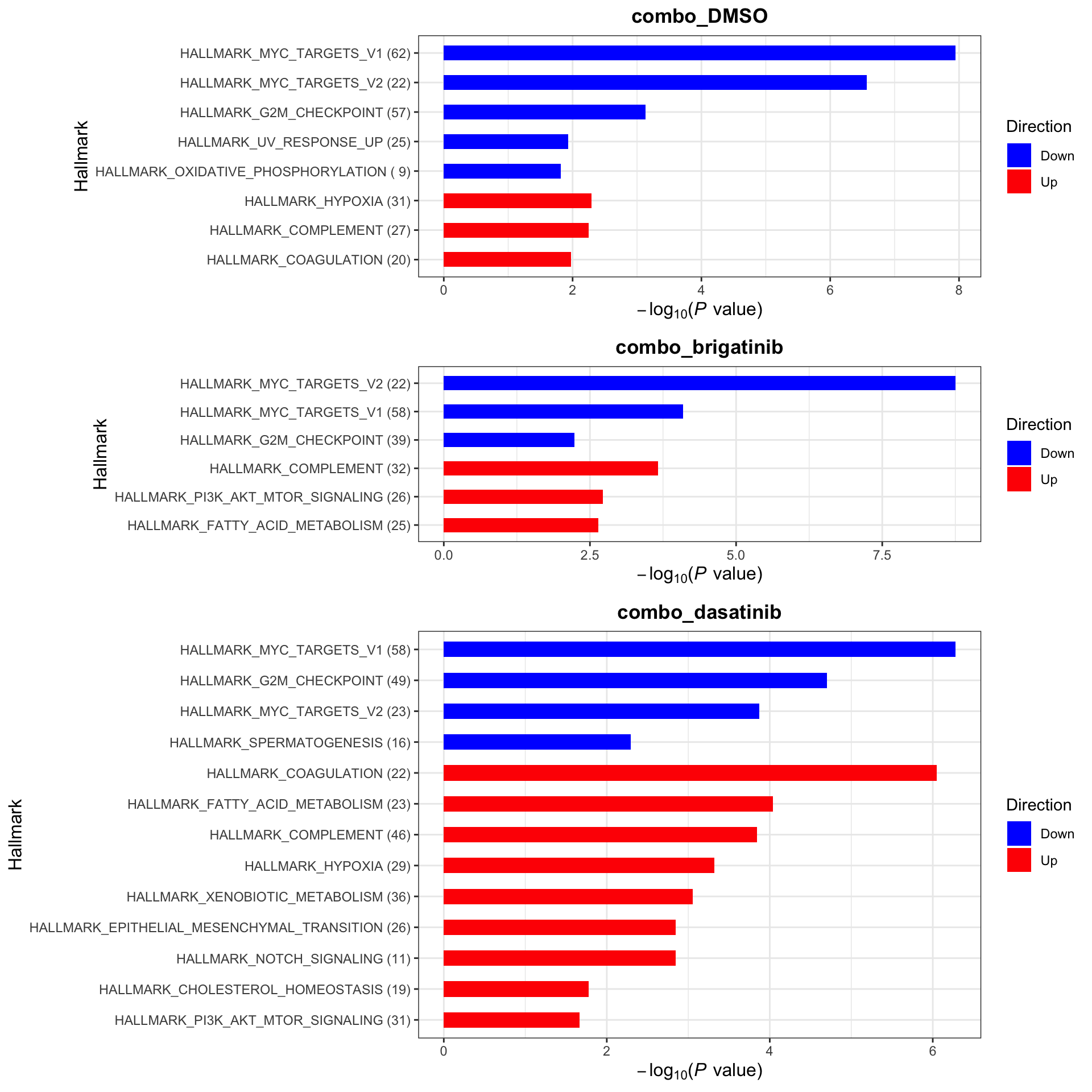
Canonical pathways
plotList$CanonicalPathway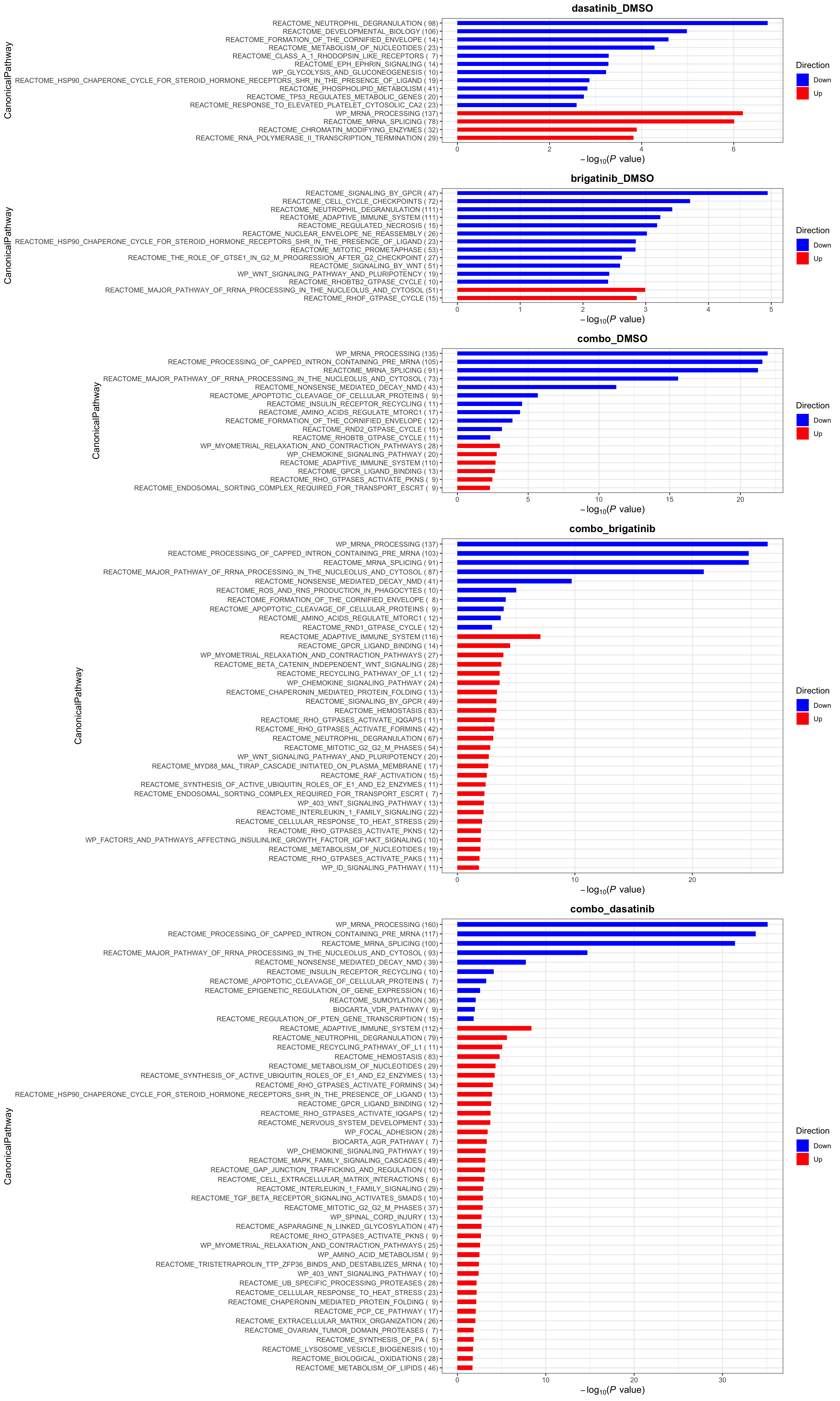
List of leading edge genes for each pathway
DT::datatable(plotList$leadingEdgeGene)writexl::write_xlsx(plotList$leadingEdgeGene, path = "../docs/enrichment_tables/prot_gsea_0.16_noMito.xlsx")Focuse on the combination effect between Brigatinib and Dasatinib (Interaction effect)
Since Brigatinib and Dasatinib has synergistic effect on cell survival, this part is to detect the synergistic effect also on protein expression level. In statistical term, this is an interaction effect, where the effect of two variables is beyond symbol linear additive effect.
Differential test
Used save results
resTab <- allResList$diffProt$time_0.17 %>% filter(compare =="interaction")
resTab.sig <- filter(resTab, adj_pval <=0.1)PCA plot with proteins showing interactions
PCA
PC1 versus PC2
plotPCA(fpeSub[resTab.sig$name,], assayName = "imputed", "PC1", "PC2", label ="replicate")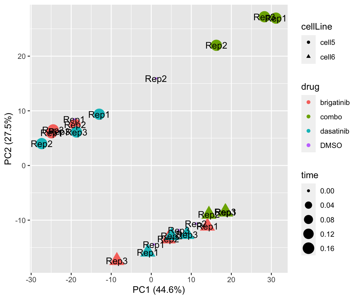 Potential problem with 1 replicate
PC3 versus PC4
plotPCA(fpeSub[resTab.sig$name,], assayName = "imputed", "PC3", "PC4", label ="replicate")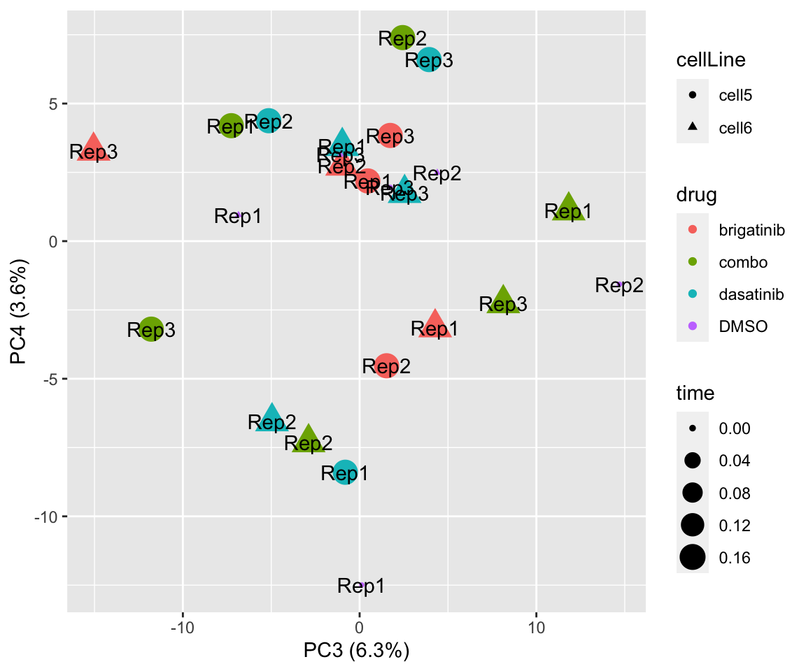
Boxplot of top 20 examples
plotTab <- jyluMisc::sumToTidy(fpeSub)
plotList <- lapply(seq(nrow(resTab.sig)), function(i) {
rec <- resTab.sig[i,]
eachTab <- filter(plotTab, rowID == rec$name)
ggplot(eachTab, aes(x=drug, y=Intensity)) +
geom_boxplot(aes(fill = drug)) +
ggbeeswarm::geom_quasirandom() +
facet_wrap(~cellLine) +
theme(legend.position = "none") +
ggtitle(rec$symbol)
})
cowplot::plot_grid(plotlist = plotList[1:20], ncol=2)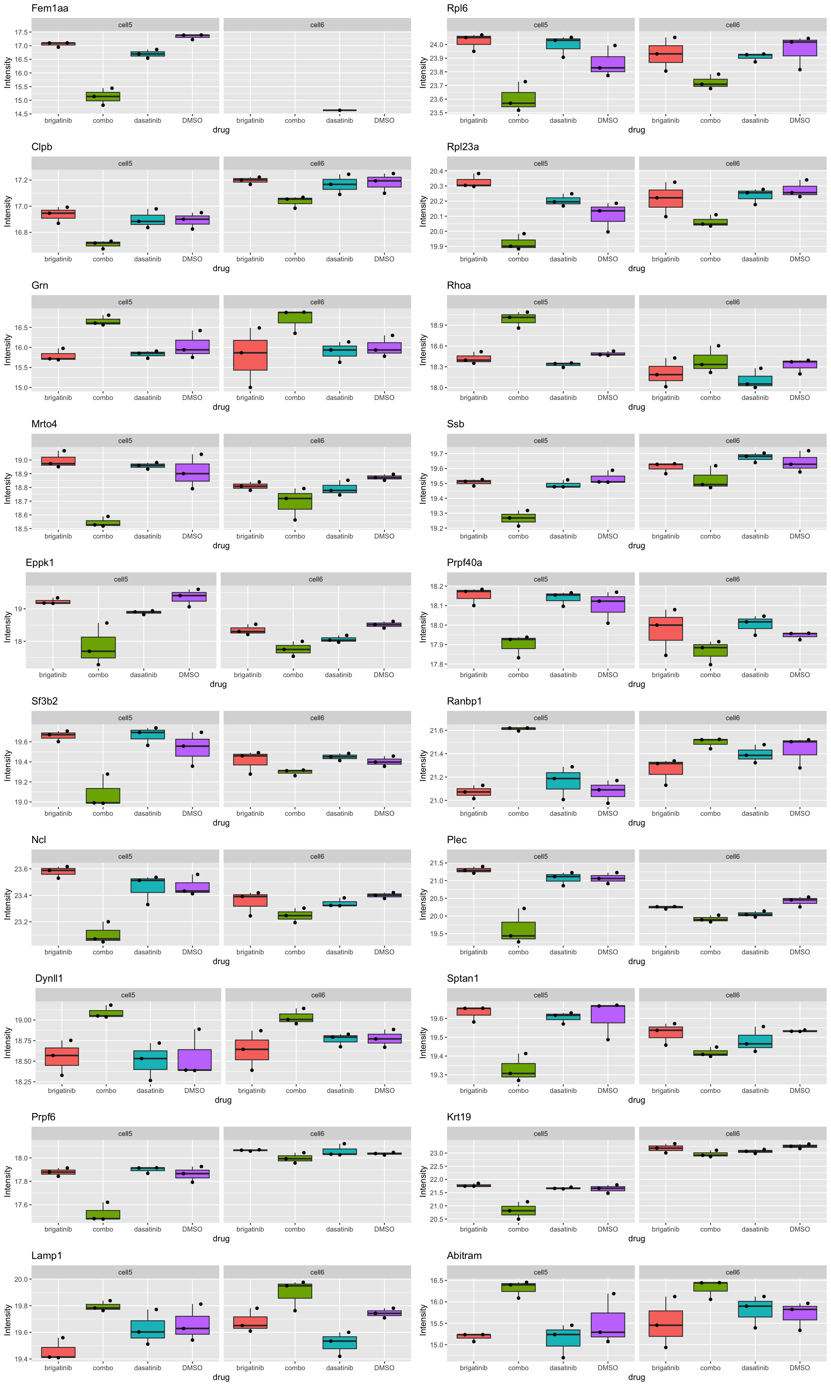
#plot all case in pdf file
#jyluMisc::makepdf(plotList, "../docs/boxplot_interaction_0.17_RUN5.pdf", ncol = 2, nrow =5, height = 15, width = 10)Download the pdf file for all significant interactions:
pdf file
Heatmap of top 100 examples
plotProteinHeatmap(resTab, fpeSub, "all", fdrCut = 0.1, ifFDR = TRUE)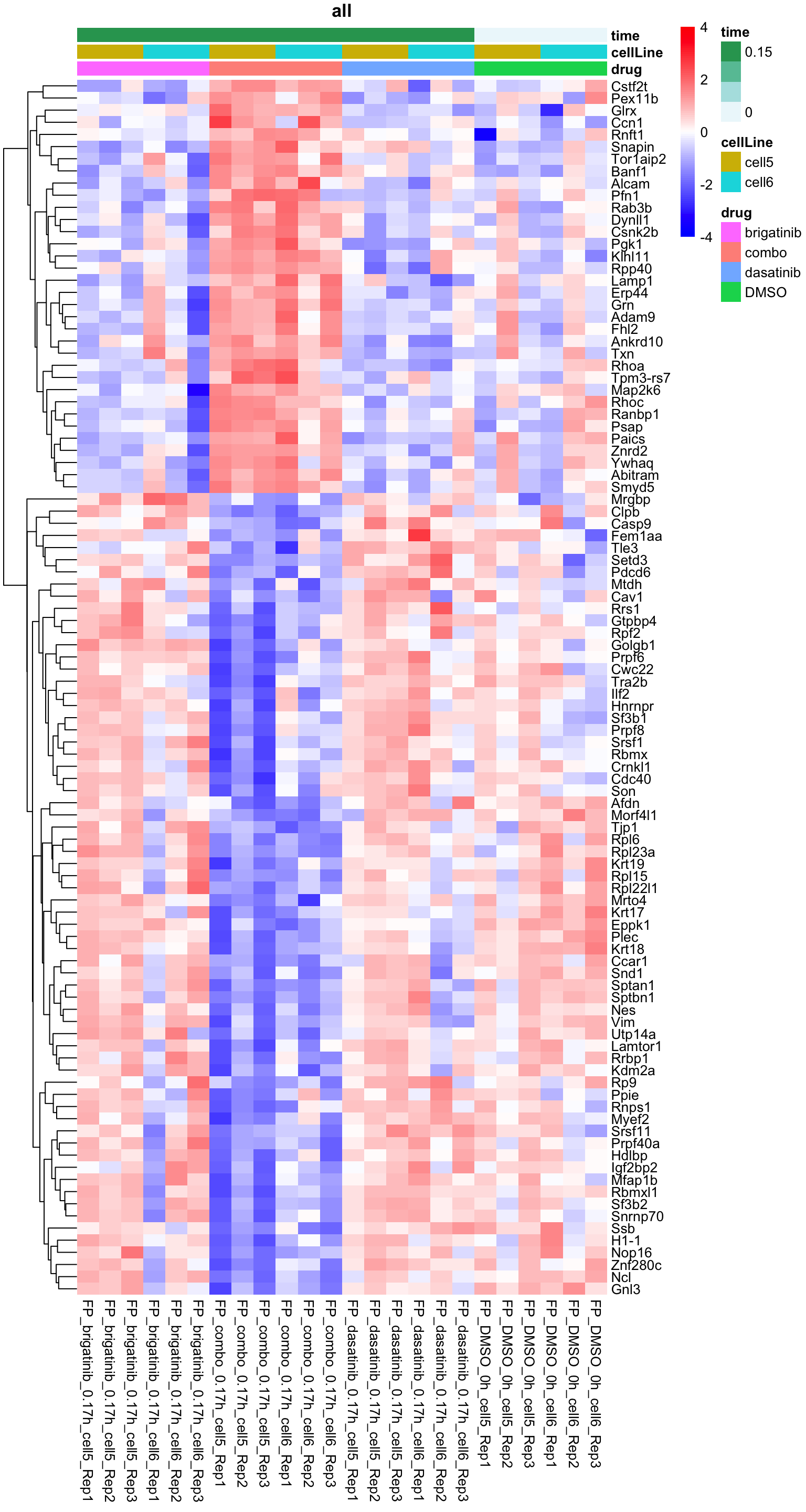
Gene set enrichment analysis
Define useful genesets
plotList <- runGeneSetEnrichment(resTab, gmts, genePCut = 1, pCutSet = 0.1, setFdr = TRUE, method="gsea", collapsePathway = TRUE)[1] "Testing for: Hallmark"
[1] "Condition: interaction"
[1] "Testing for: CanonicalPathway"
[1] "Condition: interaction"Hallmarks
plotList$Hallmark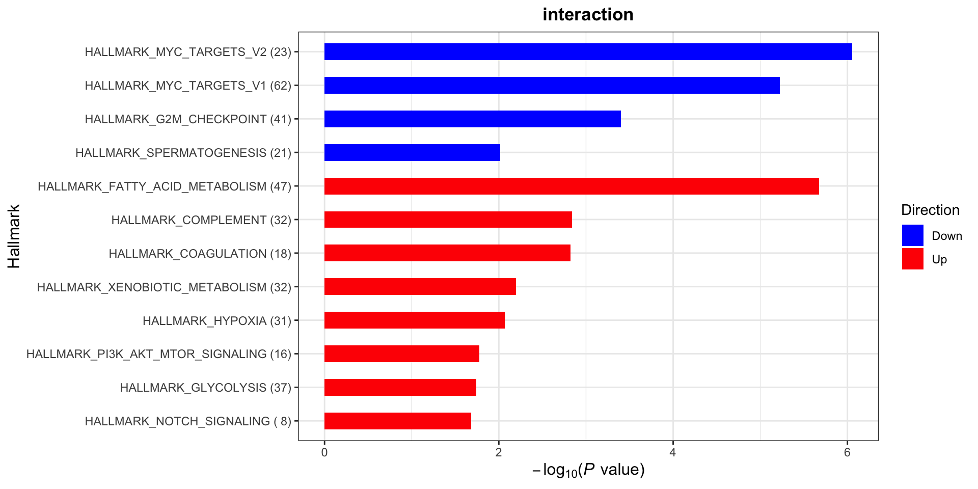
Canonical pathways
plotList$CanonicalPathway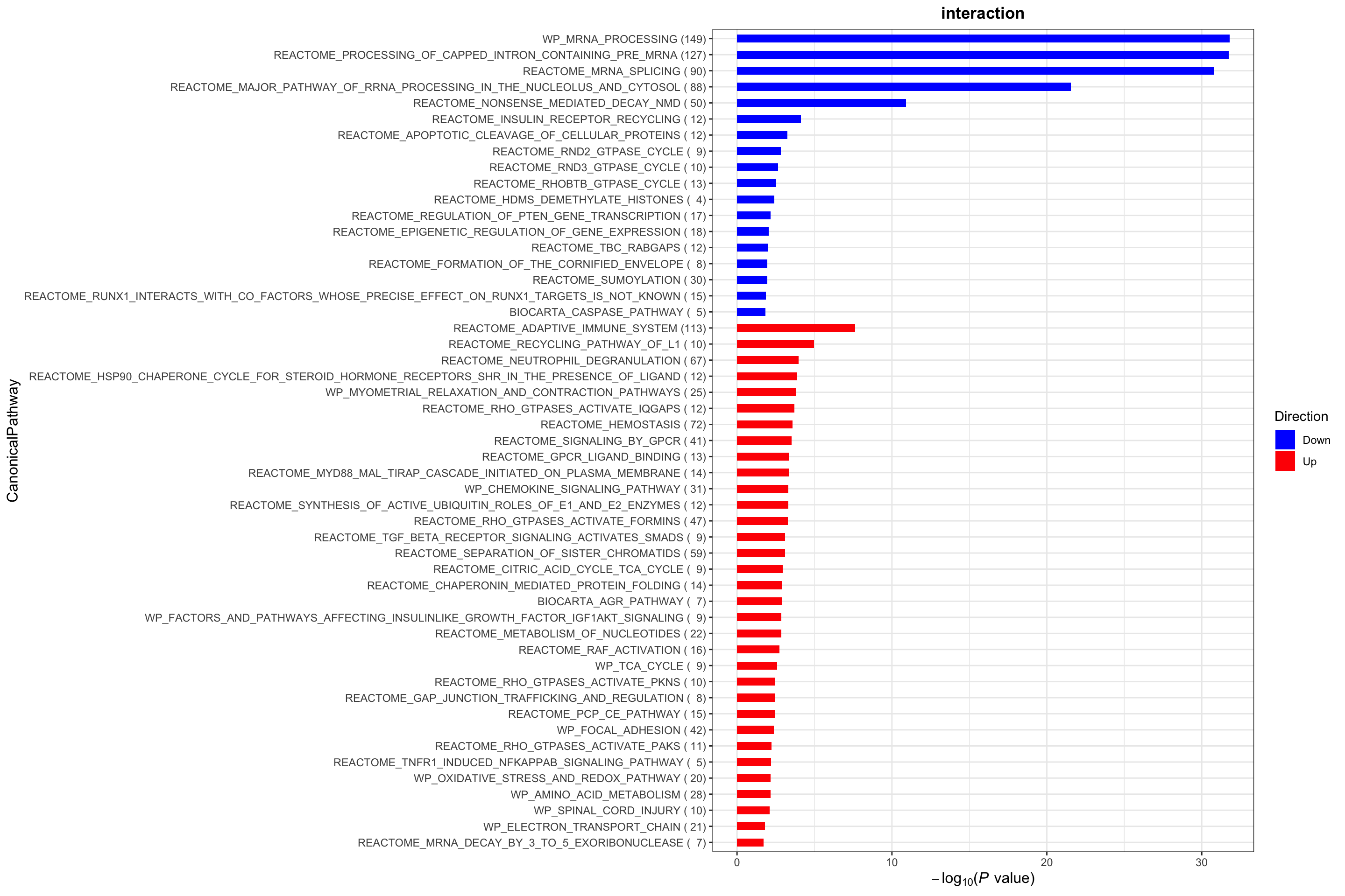
List of leading edge genes for each pathway
DT::datatable(plotList$leadingEdgeGene)writexl::write_xlsx(plotList$leadingEdgeGene, path = "../docs/enrichment_tables/prot_gsea_0.16combo.xlsx")Gene set enrichment analysis without mitocondrial genes
Define useful genesets
plotList <- runGeneSetEnrichment(filter(resTab, !symbol %in% mitoList) , gmts, genePCut = 1, pCutSet = 0.05, setFdr = TRUE, method="gsea", collapsePathway = TRUE)[1] "Testing for: Hallmark"
[1] "Condition: interaction"
[1] "Testing for: CanonicalPathway"
[1] "Condition: interaction"Hallmarks
plotList$Hallmark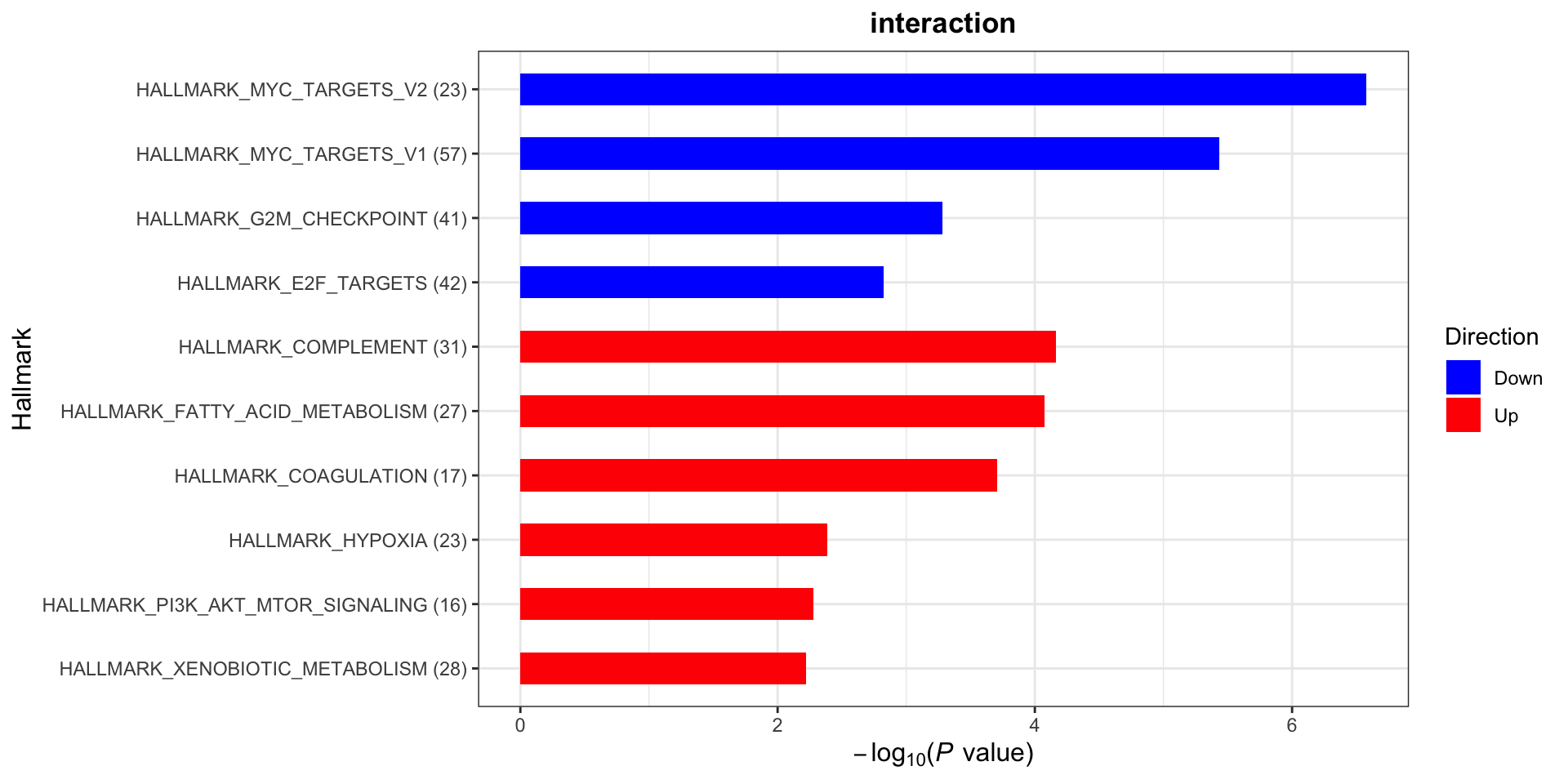
Canonical pathways
plotList$CanonicalPathway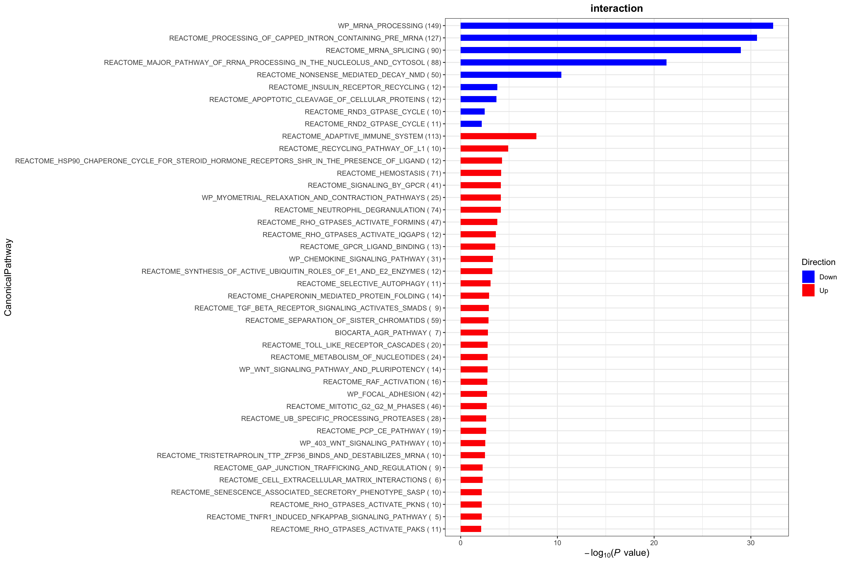
List of leading edge genes for each pathway
DT::datatable(plotList$leadingEdgeGene)writexl::write_xlsx(plotList$leadingEdgeGene, path = "../docs/enrichment_tables/prot_gsea_0.16combo_noMito.xlsx")Plot interesting pathways
HALLMARK_APOPTOSIS
All conditions will be included, difference among cell lines will be regressed out for better visualization
plotSetHeatmap(fpeSub, filter(resTab, pval < 0.05), drugPair = "all", gmtFile = gmts$Hallmark,
setName = "HALLMARK_APOPTOSIS")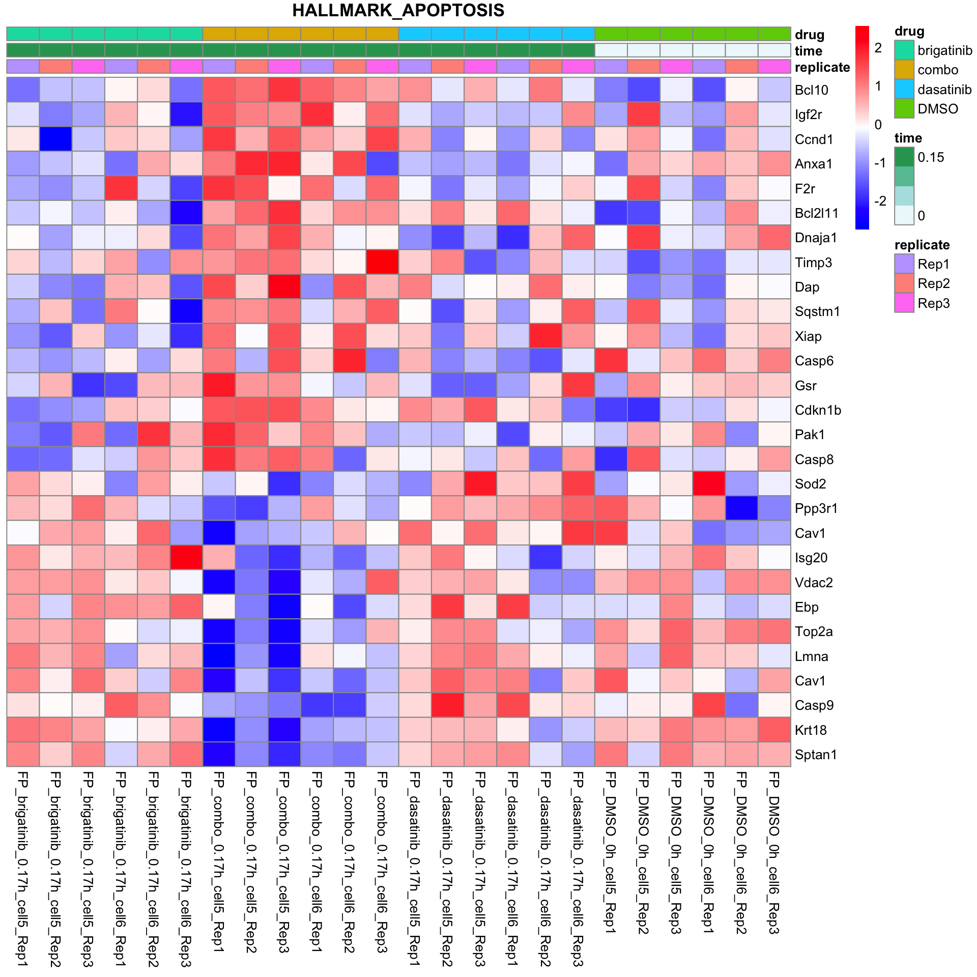
REACTOME_APOPTOTIC_CLEAVAGE_OF_CELLULAR_PROTEINS
plotSetHeatmap(fpeSub, filter(resTab, pval < 0.05), drugPair = "all", gmtFile = gmts$CanonicalPathway,
setName = "REACTOME_APOPTOTIC_CLEAVAGE_OF_CELLULAR_PROTEINS")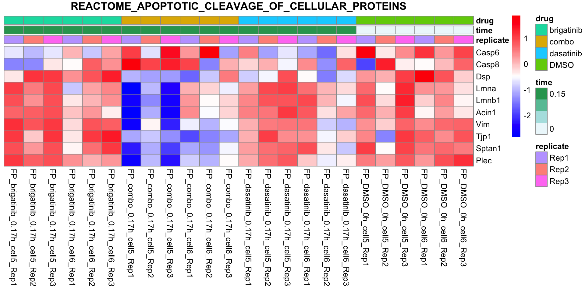
BIOCARTA_CASPASE_PATHWAY
plotSetHeatmap(fpeSub, filter(resTab, pval < 0.05), drugPair = "all", gmtFile = gmts$CanonicalPathway,
setName = "BIOCARTA_CASPASE_PATHWAY")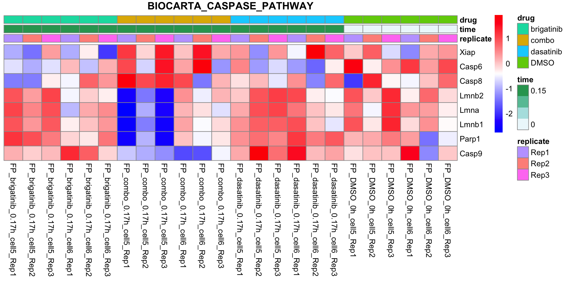
PI3K-AKT-MTOR
plotSetHeatmap(fpeSub, filter(resTab, pval < 0.05), drugPair = "all", gmtFile = gmts$Hallmark,
setName = "HALLMARK_PI3K_AKT_MTOR_SIGNALING")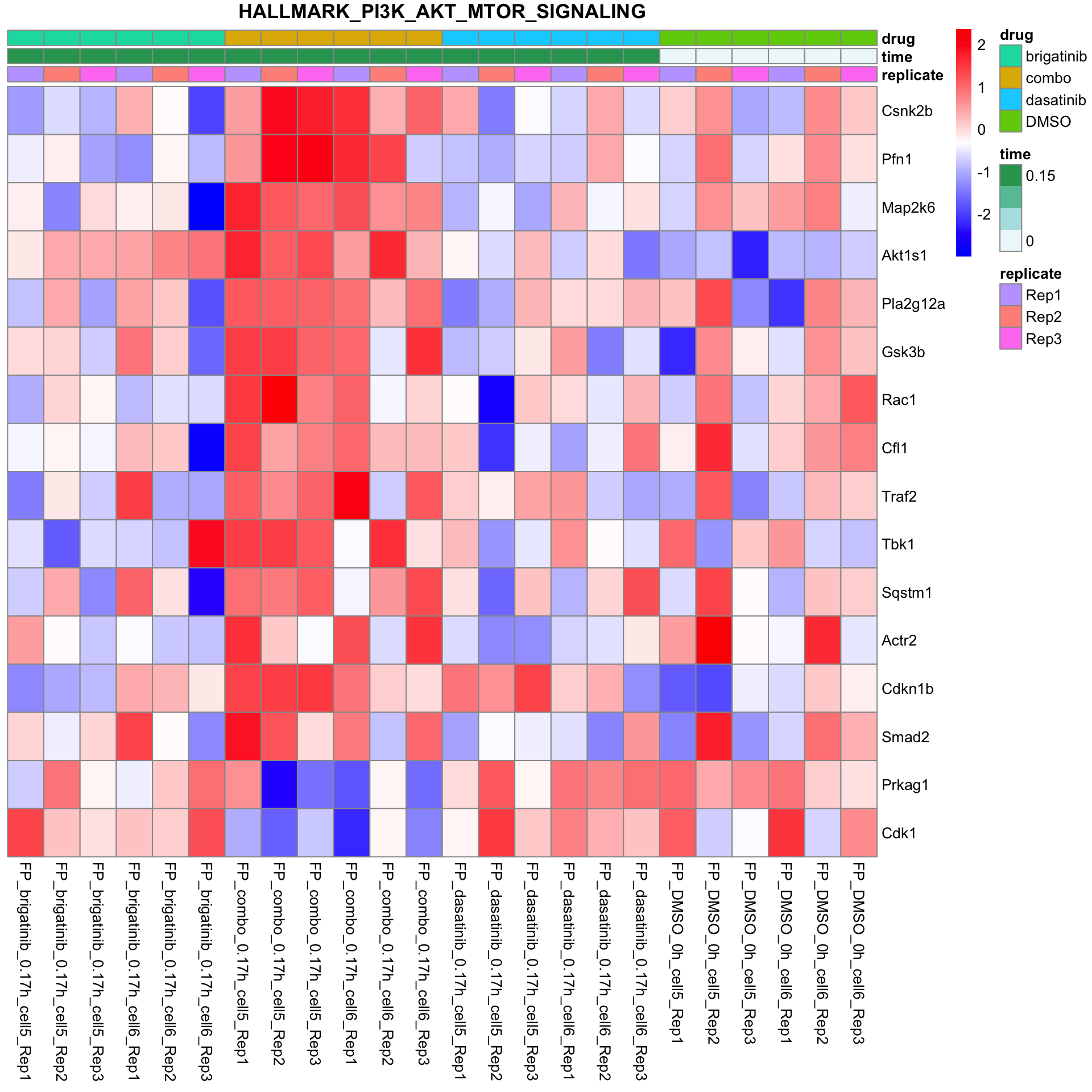
WP_MRNA_PROCESSING
plotSetHeatmap(fpeSub, filter(resTab, pval < 0.01), drugPair = "all", gmtFile = gmts$CanonicalPathway,
setName = "WP_MRNA_PROCESSING")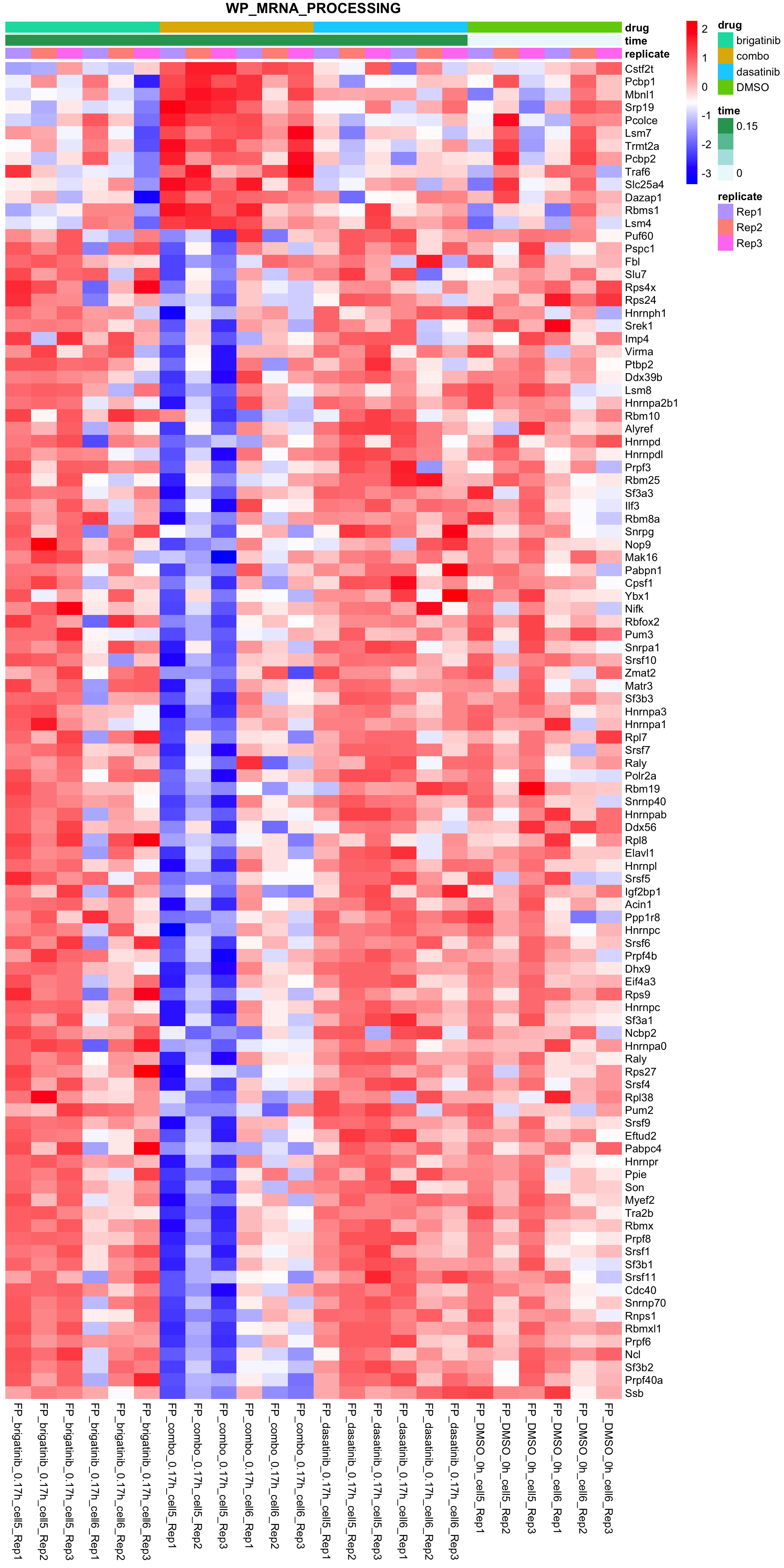
G2M_CHECKPOINT
All conditions will be included, difference among cell lines will be regressed out for better visualization
plotSetHeatmap(fpeSub, filter(resTab, pval < 0.05), drugPair = "all", gmtFile = gmts$Hallmark,
setName = "HALLMARK_G2M_CHECKPOINT")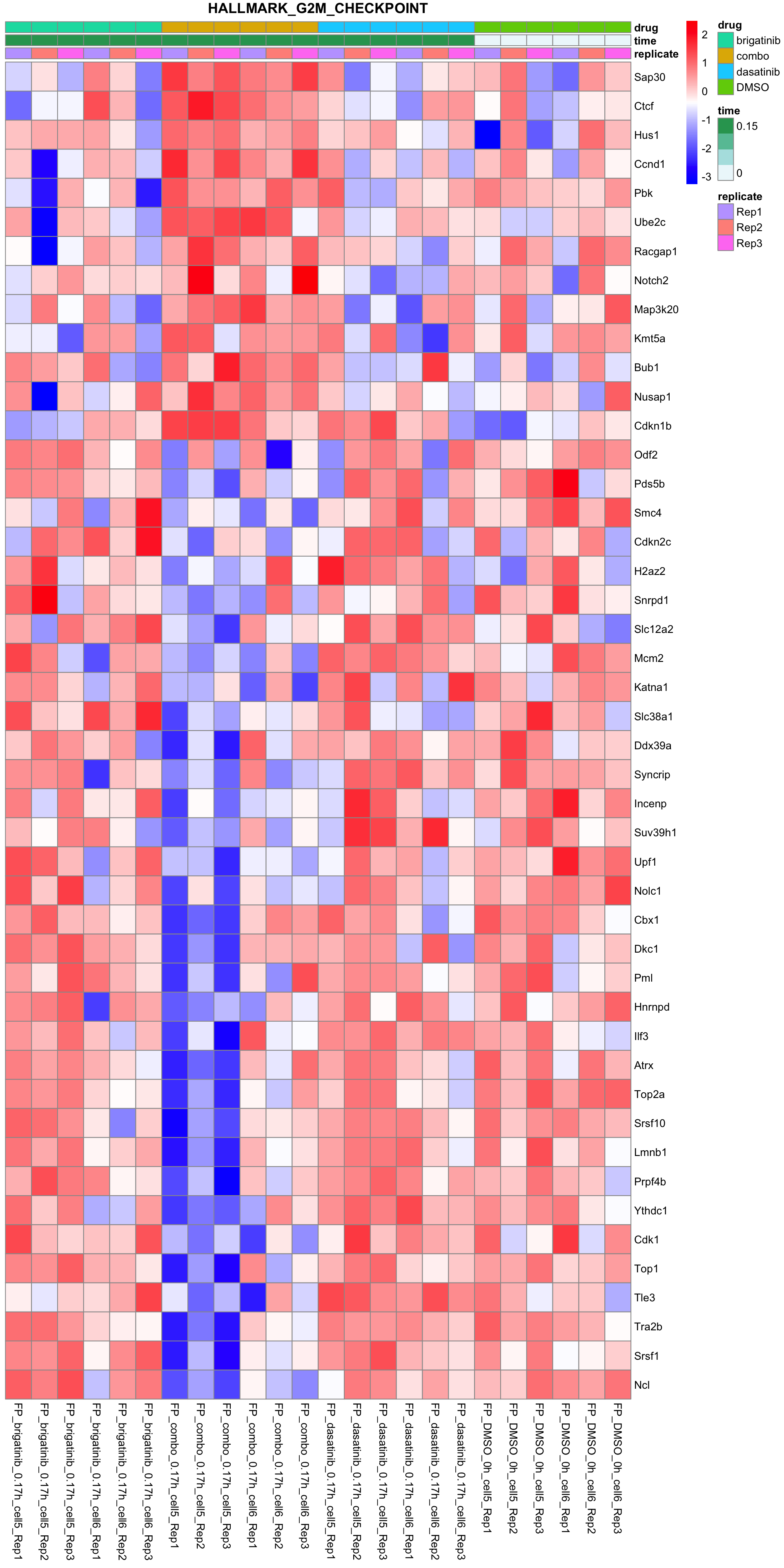
Differential expression at 16 hours for each drug
Preprocessing
filterList <- list(time = c(16,0))
fpeSub <- preprocessProteome(maeData, filterList, missCut = 0.5, transform = "vst", normalize = TRUE)[1] "Number of proteins and samples:"
[1] 7737 24Plot value distribution
plotTab <- jyluMisc::sumToTidy(fpeSub)
ggplot(plotTab, aes(x=sample, y=Intensity)) +
geom_boxplot(aes(fill = drug)) +
theme(axis.text.x = element_text(angle = 90, hjust = 1, vjust = 0.5))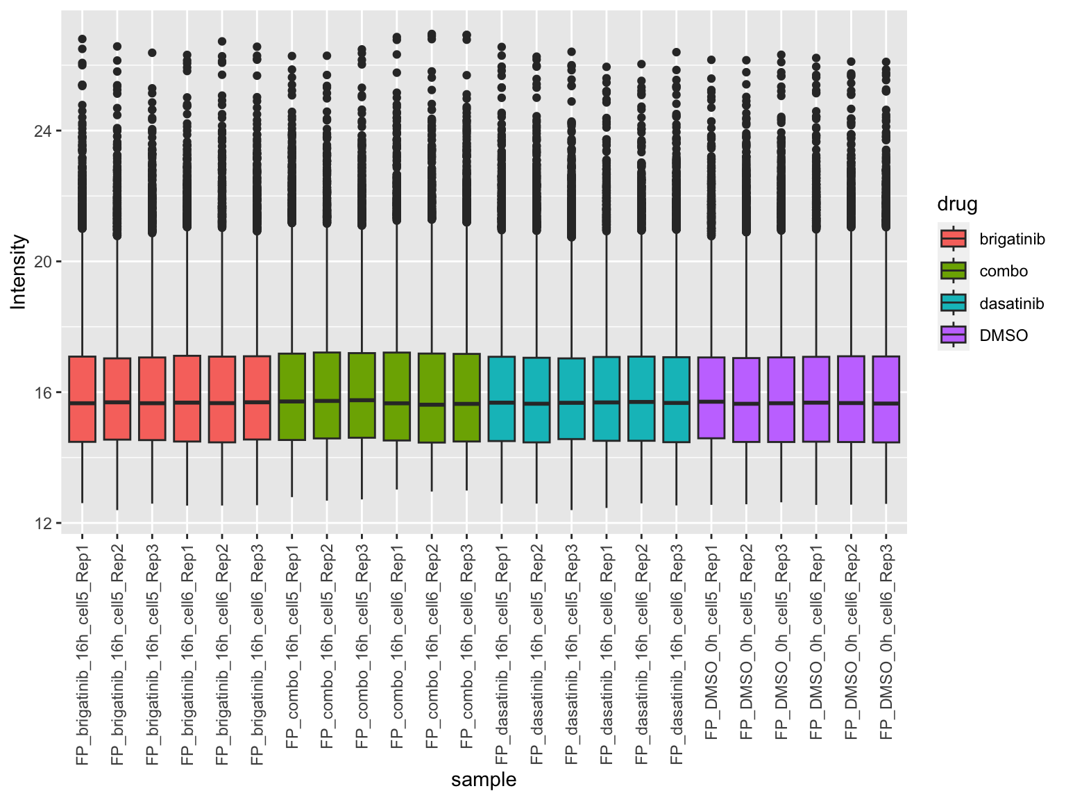
Expression of mitocondrial proteins
mitoList <- readxl::read_xls("../data/Mouse.MitoCarta3.0.xls", sheet = 2)$Symbol
plotMitoTab <- filter(plotTab, Gene %in% mitoList)
ggplot(plotMitoTab, aes(x=sample, y=Intensity)) +
geom_boxplot(aes(fill = drug)) +
theme(axis.text.x = element_text(angle = 90, hjust = 1, vjust = 0.5))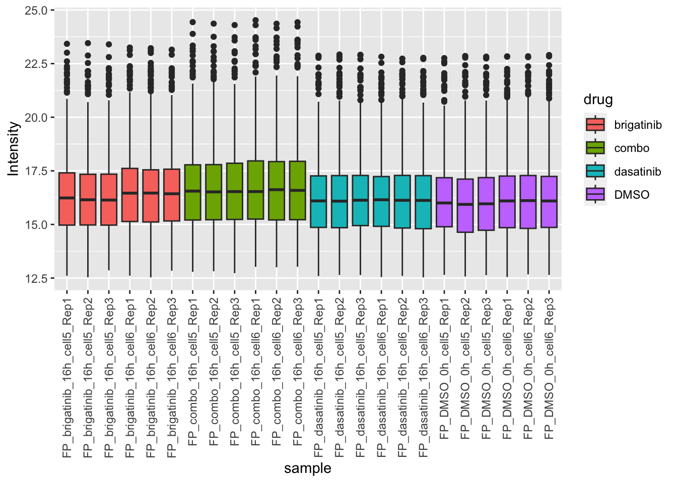 Combo treatment has slightly higher mitochondrial protein expression
PCA
PC1 versus PC2
plotPCA(fpeSub, assayName = "imputed", "PC1", "PC2", topVar = 5000, label ="replicate")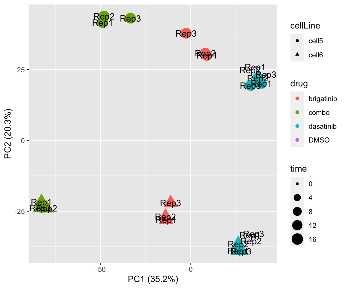 Potential problem with 1 replicate
PC3 versus PC4
plotPCA(fpeSub, assayName = "imputed", "PC3", "PC4", topVar = 5000, label = "replicate")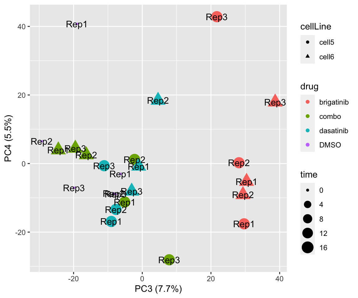
Differential expression using proDA
Use saved results
resTab <- allResList$diffProt$time_16 %>% filter(compare !="interaction")Table of significant associations (1% FDR)
Here I used 1% FDR, otherwise there are too many proteins
resTab.sig <- filter(resTab, adj_pval <= 0.01)
resTab.sig %>% mutate(across(where(is.numeric), formatC, digits=2)) %>% DT::datatable()P-value histogram for each comparison
ggplot(resTab, aes(x=pval)) +
geom_histogram(bins = 20, fill = "lightblue", color = "grey50") +
facet_wrap(~compare)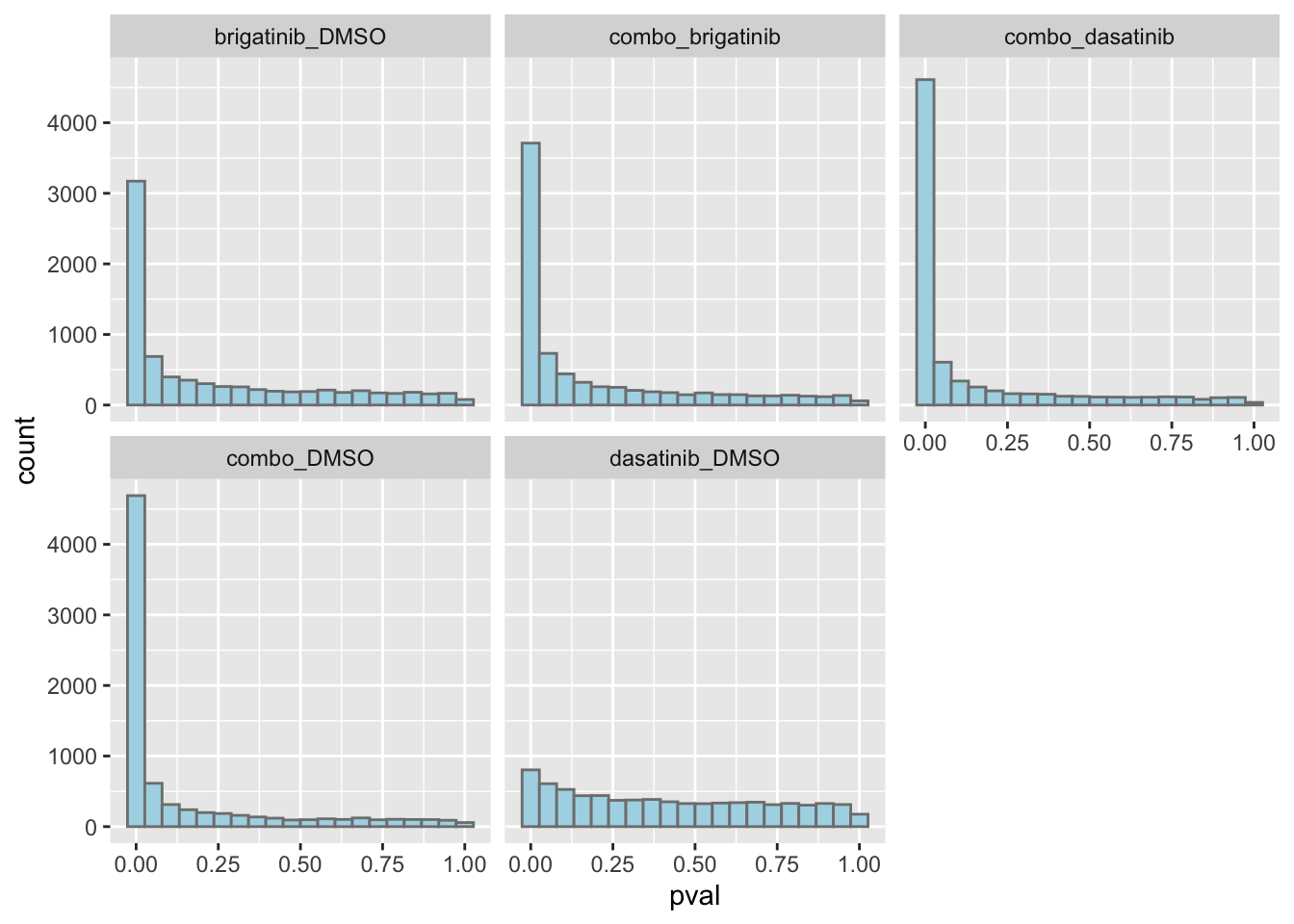
Number of DE proteins for each comparison (1% FDR)
sumTab <- filter(resTab, adj_pval < 0.01) %>%
mutate(direction = ifelse(diff>0, "Up","Down")) %>%
group_by(compare, direction) %>%
summarise(n=length(name))
ggplot(sumTab, aes(x=compare, y=n)) +
geom_bar(aes(fill = direction), stat = "identity", position = "dodge") +
coord_flip() +
geom_text(aes(label =n)) +
facet_wrap(~direction, ncol=2, scales = "free_x") +
xlab("Number")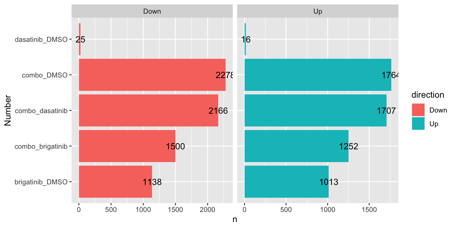
Number of mitochondrial DE proteins for each comparison (1% FDR)
sumTab <- filter(resTab, adj_pval < 0.01, symbol %in% mitoList) %>%
mutate(direction = ifelse(diff>0, "Up","Down")) %>%
group_by(compare, direction) %>%
summarise(n=length(name))
ggplot(sumTab, aes(x=compare, y=n)) +
geom_bar(aes(fill = direction), stat = "identity", position = "dodge") +
coord_flip() +
geom_text(aes(label =n)) +
facet_wrap(~direction, ncol=2, scales = "free_x") +
xlab("Number")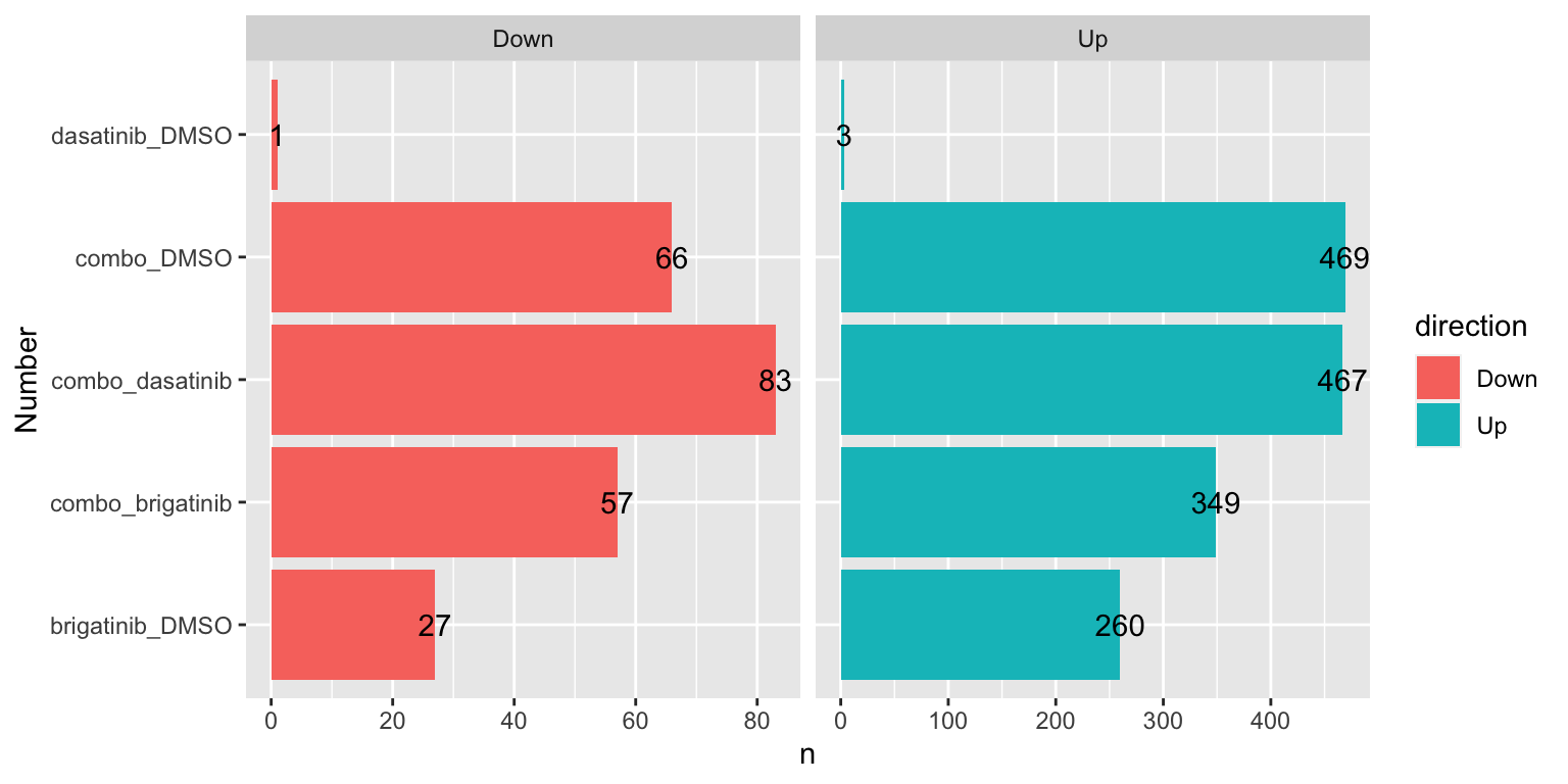 Quite a lot mitochondrial proteins are involved.
Heatmap of DE proteins for each treatment
Brigatinib versus DMSO
plotProteinHeatmap(resTab, fpeSub, "brigatinib_DMSO", fdrCut = 0.01, ifFDR = TRUE)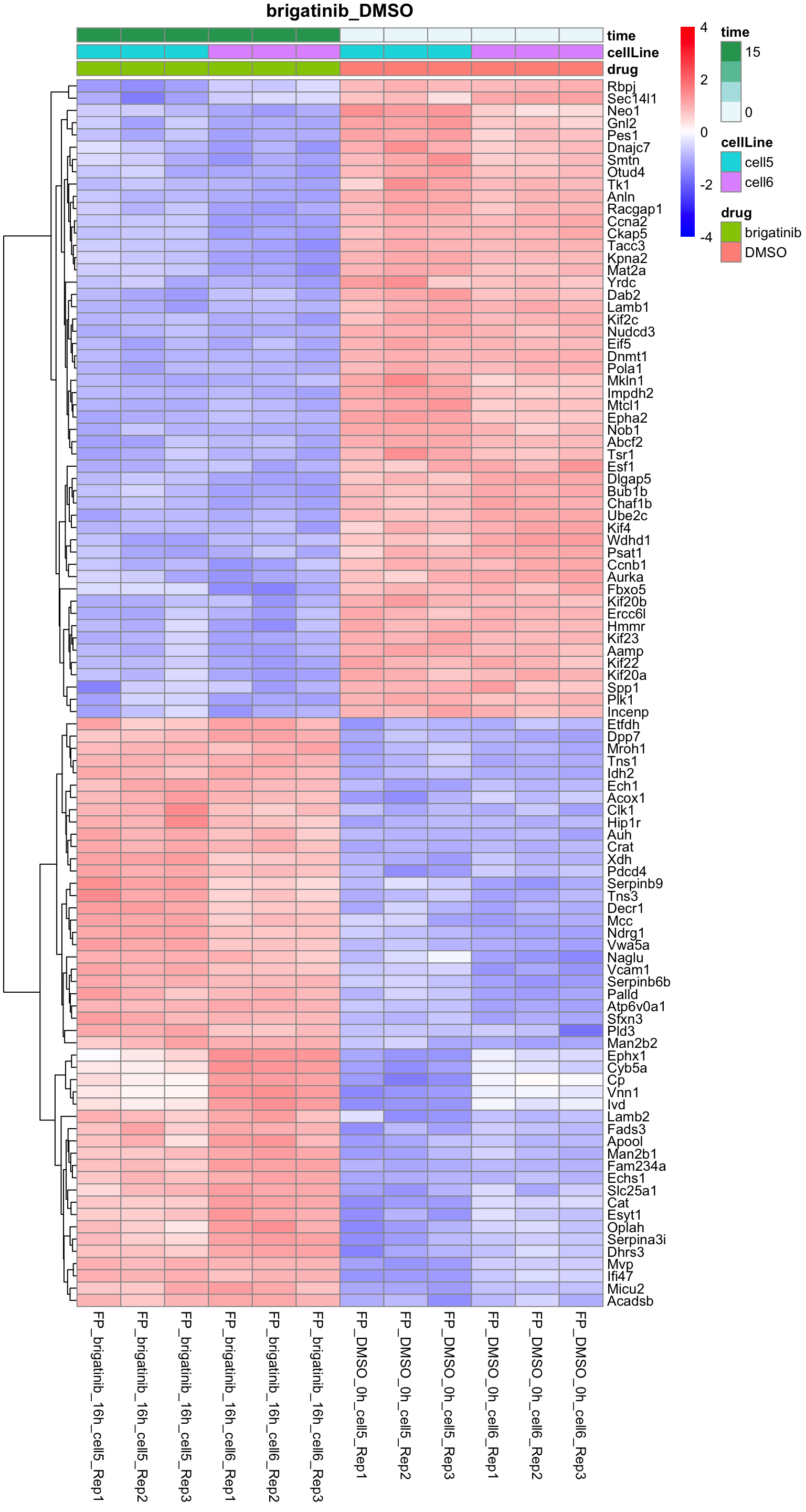
Dasatinib versus DMSO
plotProteinHeatmap(resTab, fpeSub, "dasatinib_DMSO", fdrCut = 0.01, ifFDR =TRUE)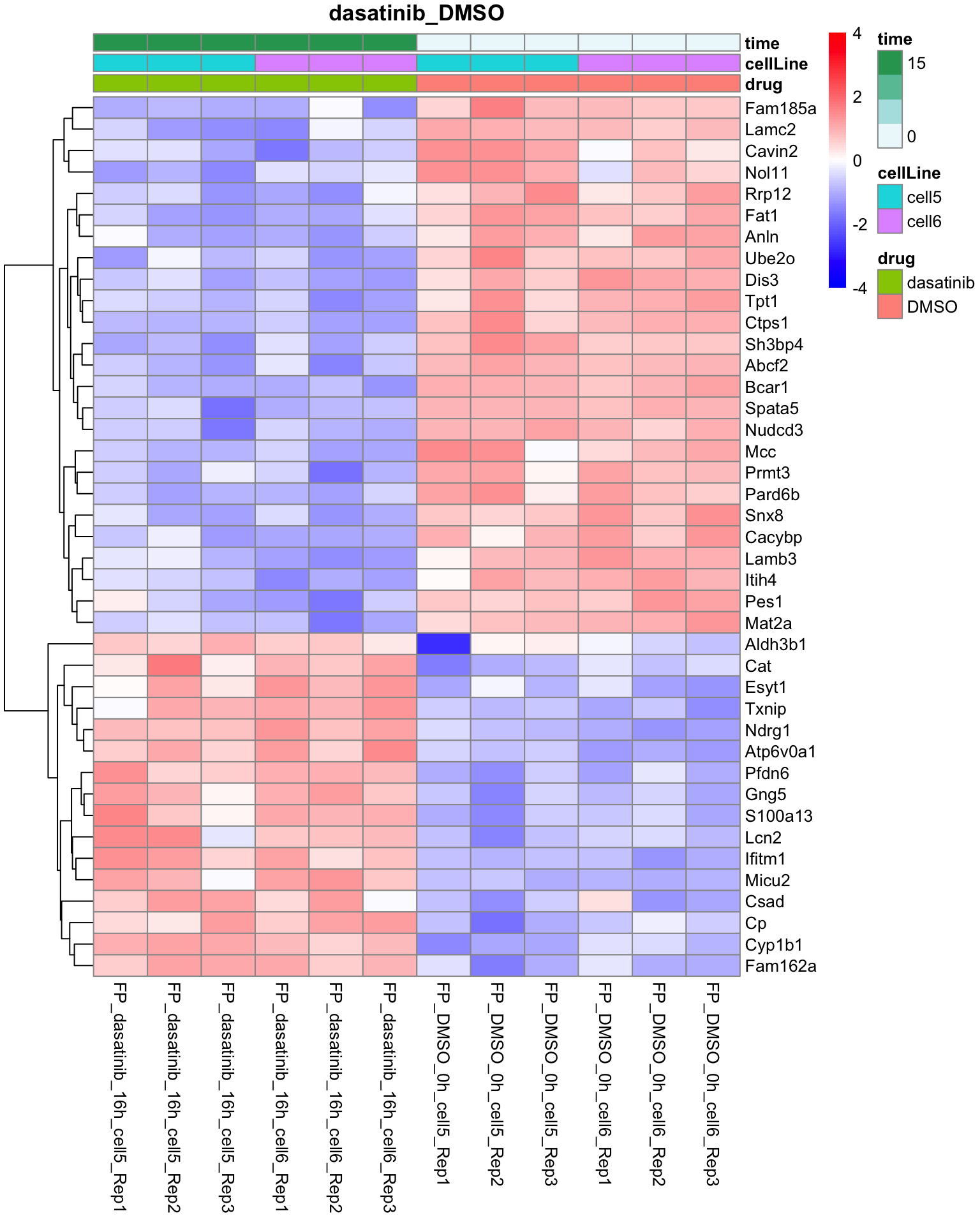
Combo versus DMSO
plotProteinHeatmap(resTab, fpeSub, "combo_DMSO", fdrCut = 0.01, ifFDR = TRUE)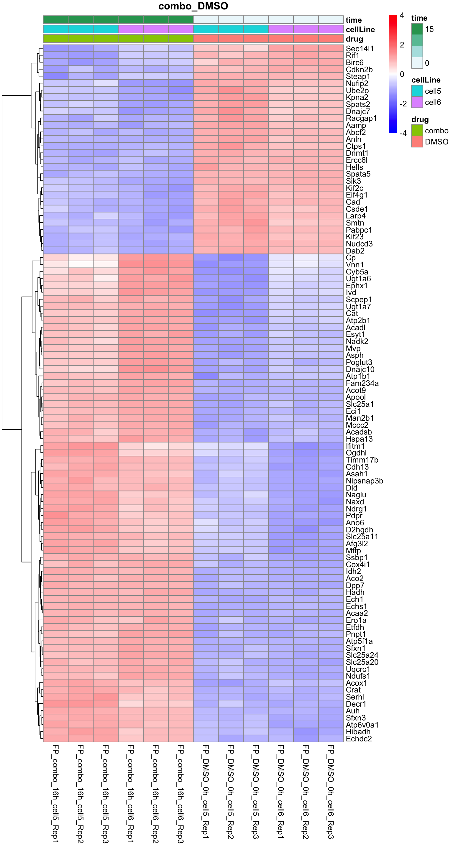
Combo versus brigatinib
plotProteinHeatmap(resTab, fpeSub, "combo_brigatinib", fdrCut = 0.01, ifFDR = TRUE)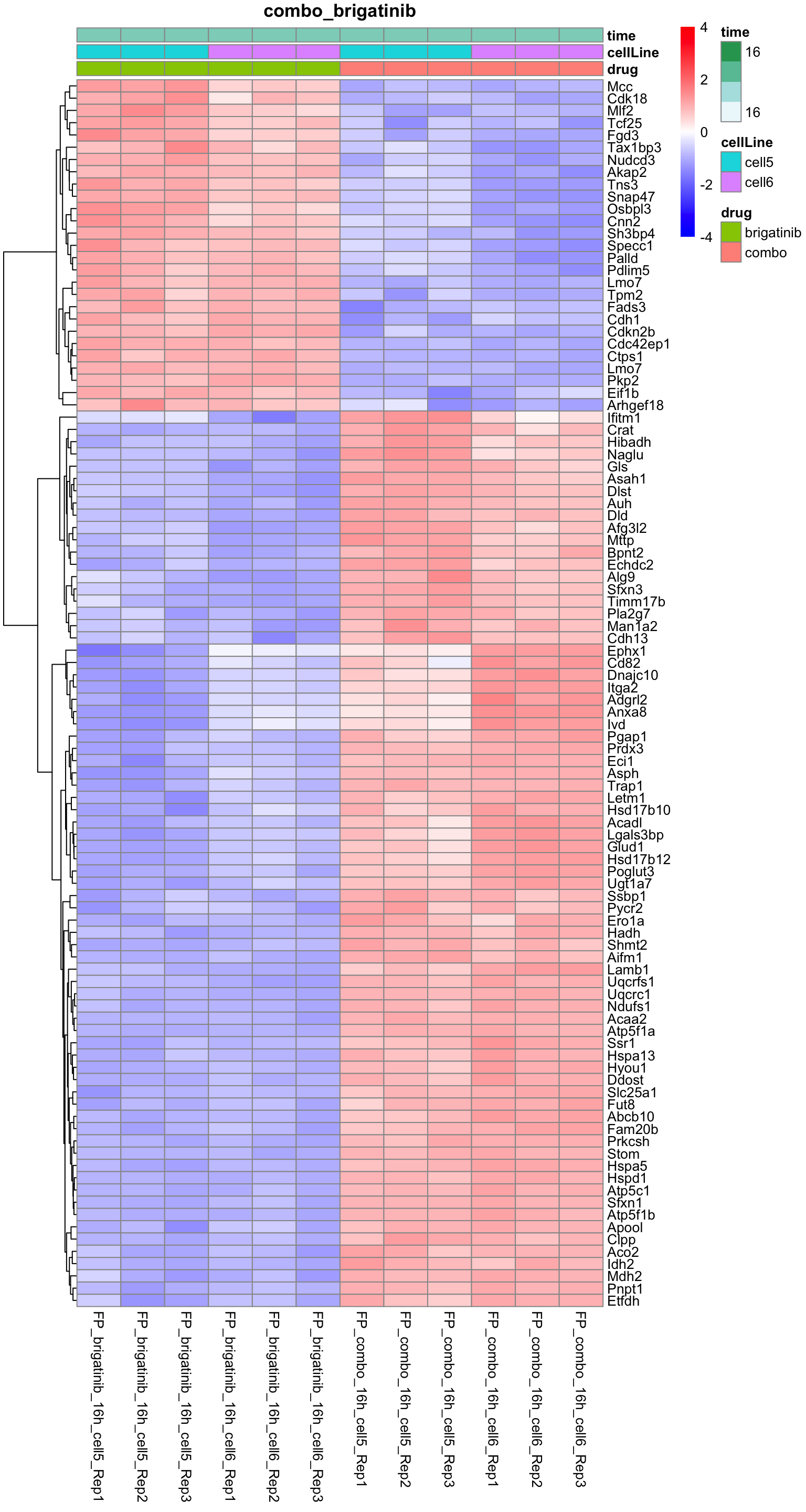
Combo versus dasatinib
plotProteinHeatmap(resTab, fpeSub, "combo_dasatinib", fdrCut = 0.01, ifFDR = TRUE)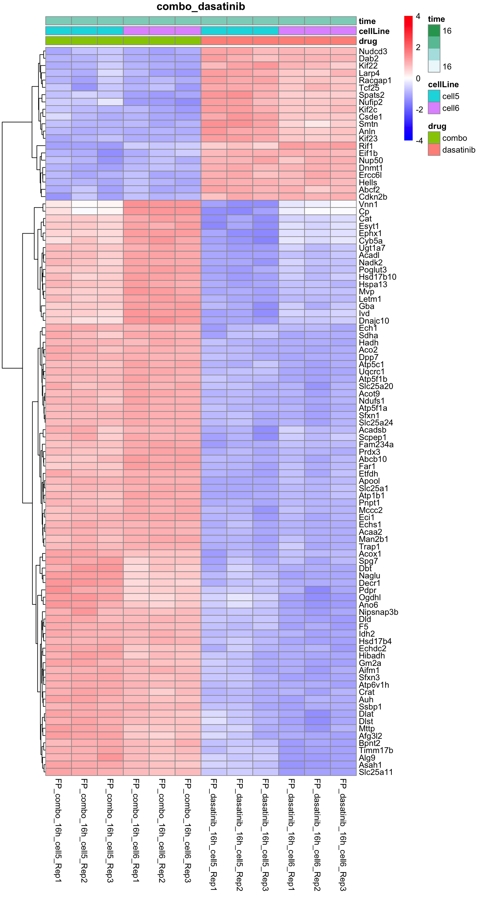
Overlap of DE proteins
Up regulated
deList <- lapply(unique(resTab$compare), function(x) {
filter(resTab, compare == x,adj_pval<0.1, diff >0)$name
})
names(deList) <- unique(resTab$compare)
upset(fromList(deList))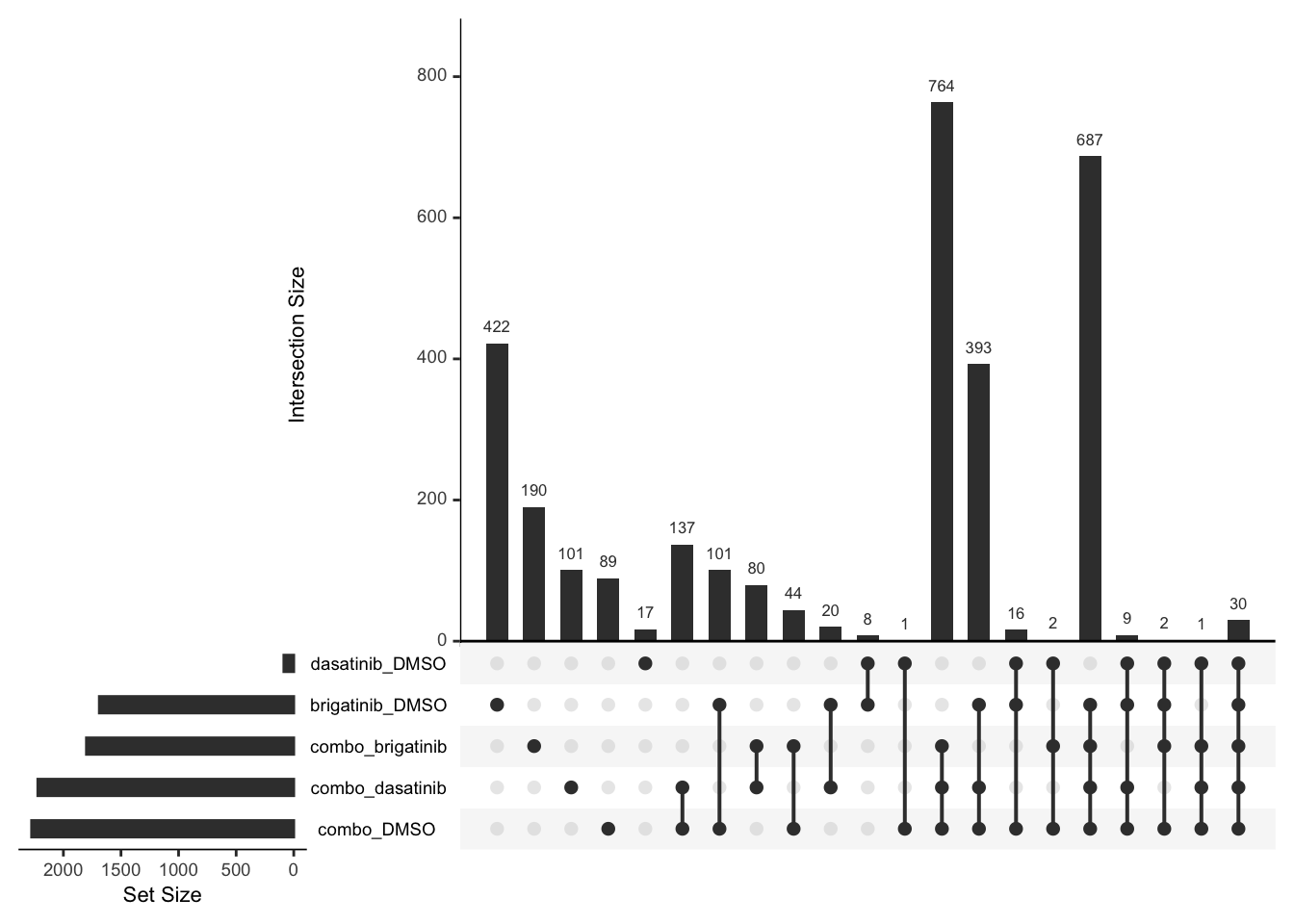
Down regulated
deList <- lapply(unique(resTab$compare), function(x) {
filter(resTab, compare == x, adj_pval <= 0.1, diff <0)$name
})
names(deList) <- unique(resTab$compare)
upset(fromList(deList))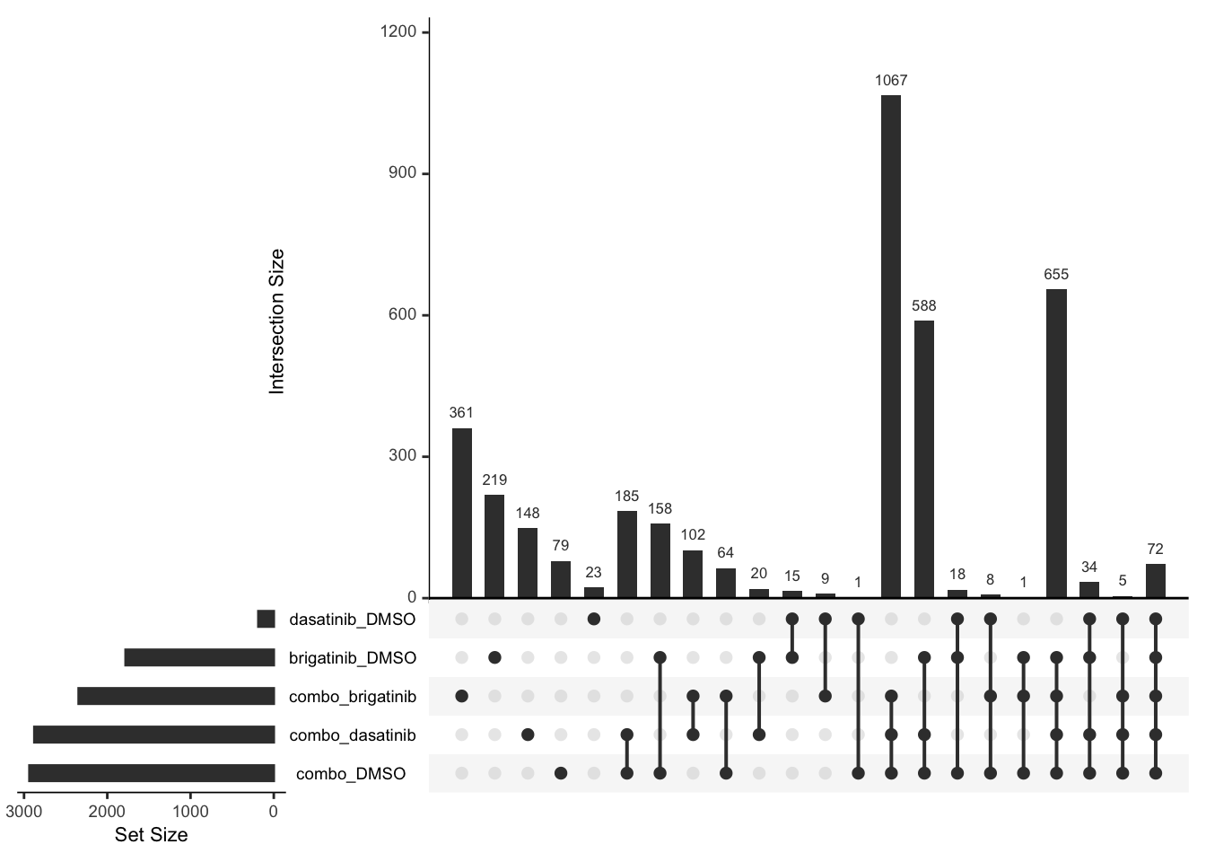
Gene set enrichment analysis
Remove mitochondrial proteins for the downstream analysis
resTab <- filter(resTab, !symbol %in% mitoList)Define useful genesets
gmts <- list(Hallmark = "../data/gmts/mh.all.v2022.1.Mm.symbols.gmt",
CanonicalPathway = "../data/gmts/m2.cp.v2022.1.Mm.symbols.gmt")
plotList <- runGeneSetEnrichment(resTab, gmts, genePCut = 1, pCutSet = 0.05, geneFdr = FALSE, setFdr = TRUE, method="gsea", collapsePathway = TRUE)[1] "Testing for: Hallmark"
[1] "Condition: dasatinib_DMSO"
[1] "Condition: brigatinib_DMSO"
[1] "Condition: combo_DMSO"
[1] "Condition: combo_brigatinib"
[1] "Condition: combo_dasatinib"
[1] "Testing for: CanonicalPathway"
[1] "Condition: dasatinib_DMSO"
[1] "Condition: brigatinib_DMSO"
[1] "Condition: combo_DMSO"
[1] "Condition: combo_brigatinib"
[1] "Condition: combo_dasatinib"Hallmarks
plotList$Hallmark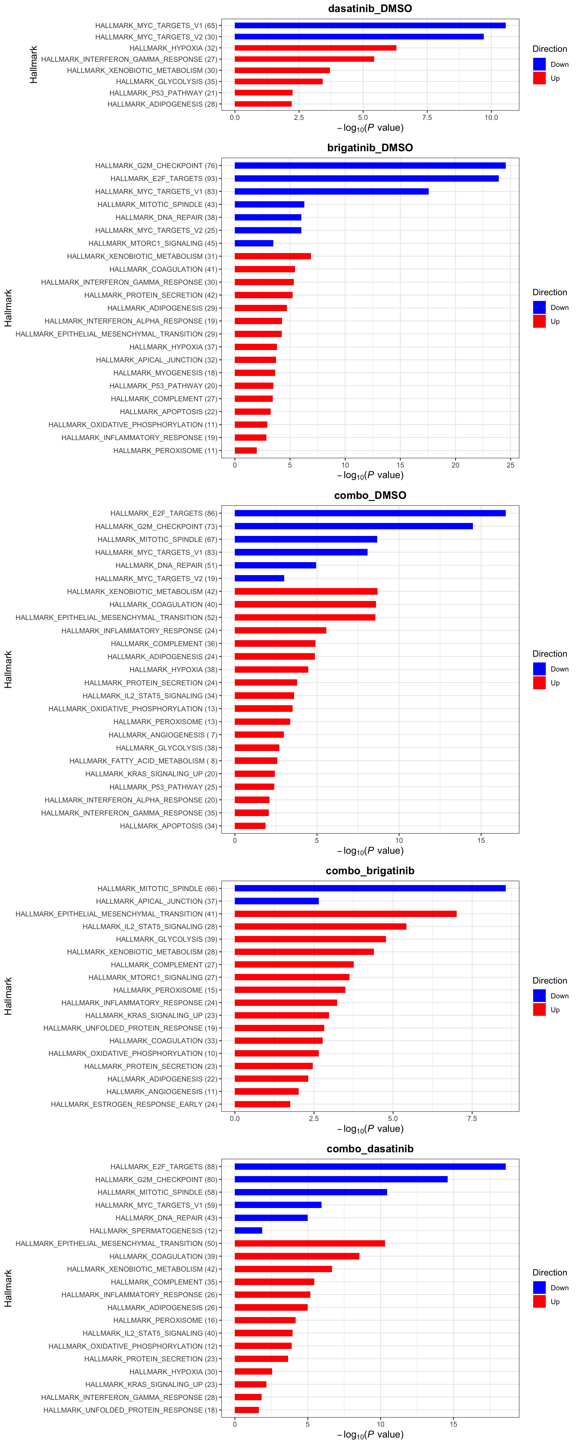
Canonical pathways
plotList$CanonicalPathway
List of leading edge genes for each pathway
DT::datatable(plotList$leadingEdgeGene)writexl::write_xlsx(plotList$leadingEdgeGene, path = "../docs/enrichment_tables/prot_gsea_16_noMito.xlsx")Focuse on the combination effect between Brigatinib and Dasatinib (Interaction effect)
Since Brigatinib and Dasatinib has synergistic effect on cell survival, this part is to detect the synergistic effect also on protein expression level. In statistical term, this is an interaction effect, where the effect of two variables is beyond symbol linear additive effect.
Differential test
Used save results, remove mitochondrial genes
resTab <- allResList$diffProt$time_16 %>% filter(compare =="interaction")
resTab.sig <- filter(resTab, adj_pval <= 0.01)Here I used 0.01 adjusted p-values, otherwise there will be too many proteins
PCA plot with proteins showing interactions
PCA
PC1 versus PC2
plotPCA(fpeSub[resTab.sig$name,], assayName = "imputed", "PC1", "PC2", label ="replicate") Potential problem with 1 replicate
PC3 versus PC4
plotPCA(fpeSub[resTab.sig$name,], assayName = "imputed", "PC3", "PC4", label ="replicate")
List of proteins with significant interactions (10%FDR)
resTab.sig %>% mutate(across(where(is.numeric), formatC, digits=2)) %>% DT::datatable()Heatmap of top 100 examples
plotProteinHeatmap(resTab, fpeSub, "all", fdrCut = 0.1, ifFDR = TRUE)
Box-Plot top 20 examples
plotTab <- jyluMisc::sumToTidy(fpeSub)
plotList <- lapply(seq(20), function(i) {
rec <- resTab.sig[i,]
eachTab <- filter(plotTab, rowID == rec$name)
ggplot(eachTab, aes(x=drug, y=Intensity)) +
geom_boxplot(aes(fill = drug)) +
ggbeeswarm::geom_quasirandom() +
facet_wrap(~cellLine) +
theme(legend.position = "none") +
ggtitle(rec$symbol)
})
cowplot::plot_grid(plotlist = plotList[1:20], ncol=2)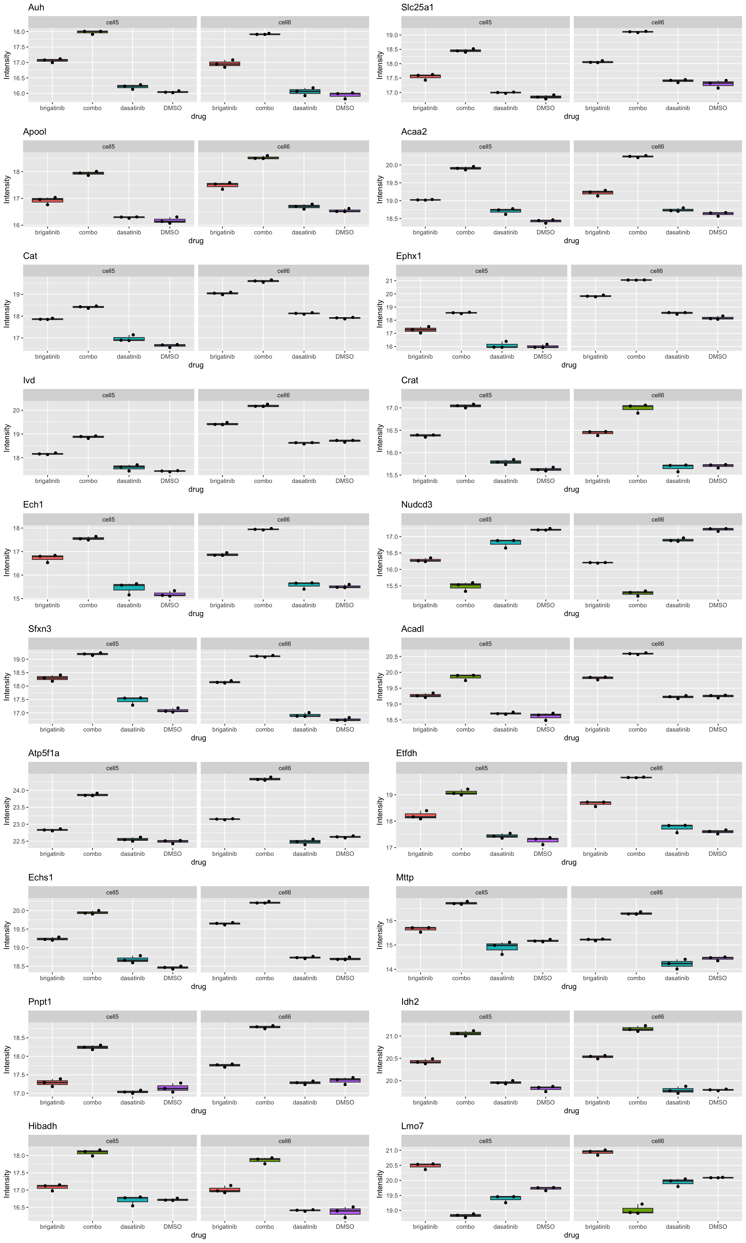 Most proteins show distinct effect in combo treatment. Doesn’t make too
much sense to plot all of them.
Most proteins show distinct effect in combo treatment. Doesn’t make too
much sense to plot all of them.
Gene set enrichment analysis
Define useful genesets
plotList <- runGeneSetEnrichment(resTab, gmts, genePCut = 1, pCutSet = 0.05, setFdr = TRUE, method="gsea", collapsePathway = TRUE)[1] "Testing for: Hallmark"
[1] "Condition: interaction"
[1] "Testing for: CanonicalPathway"
[1] "Condition: interaction"Hallmarks
plotList$Hallmark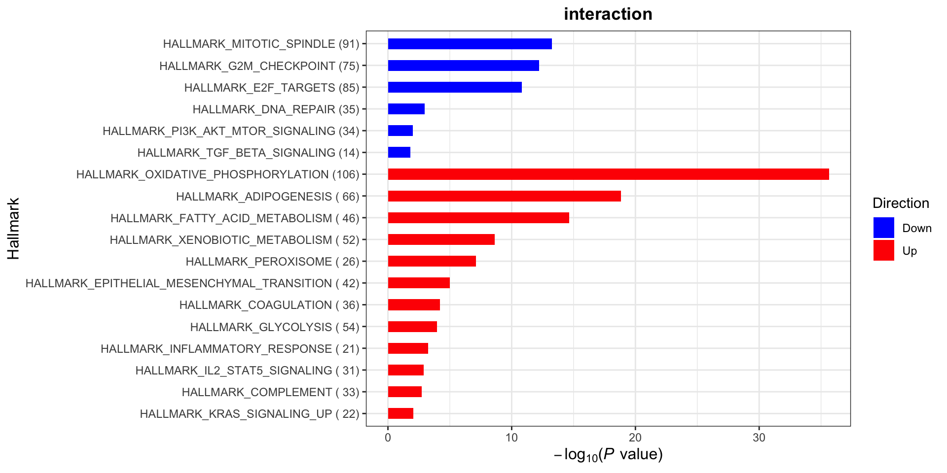
Canonical pathways
plotList$CanonicalPathway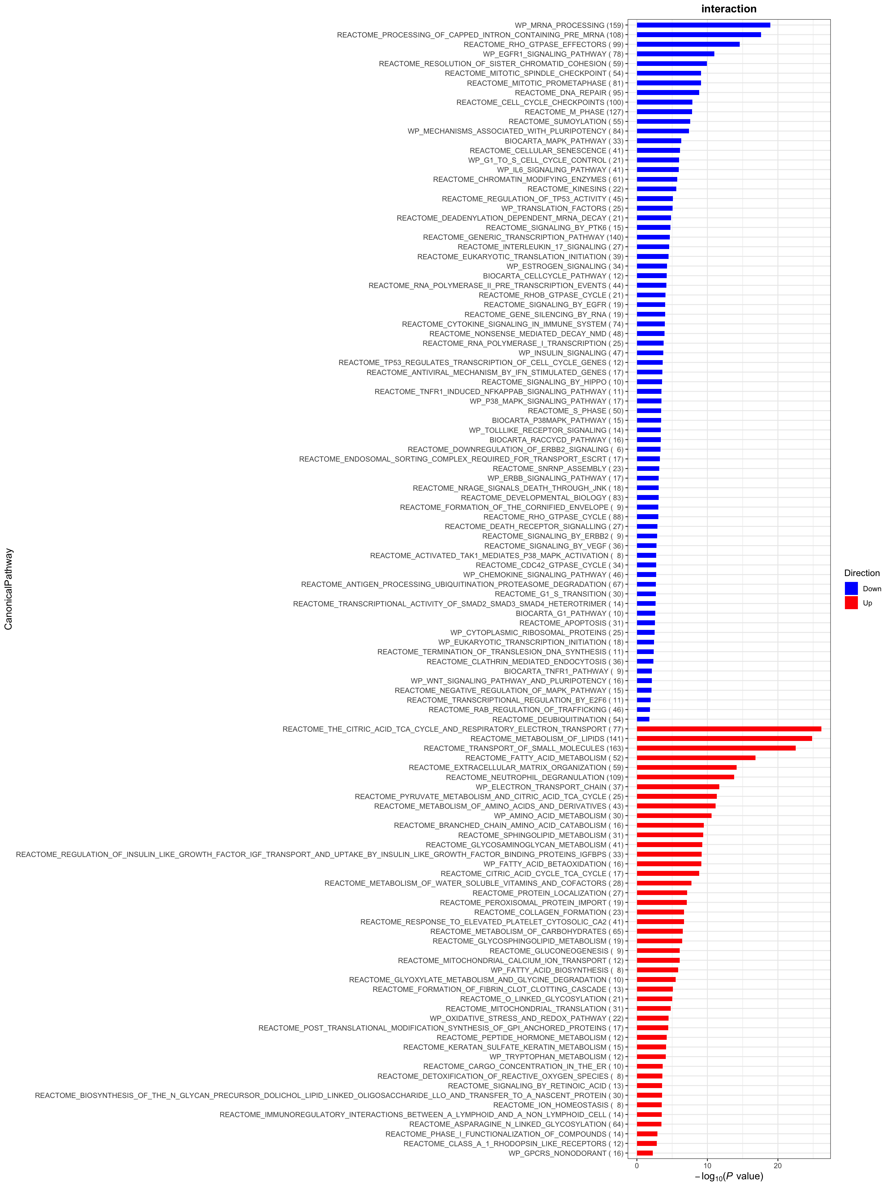
List of leading edge genes for each pathway
DT::datatable(plotList$leadingEdgeGene)writexl::write_xlsx(plotList$leadingEdgeGene, path = "../docs/enrichment_tables/prot_gsea_16combo.xlsx")Gene set enrichment analysis without mitochondrial proteins
Define useful genesets
plotList <- runGeneSetEnrichment(filter(resTab, !symbol %in% mitoList), gmts, genePCut = 1, pCutSet = 0.05, setFdr = TRUE, method="gsea", collapsePathway = TRUE)[1] "Testing for: Hallmark"
[1] "Condition: interaction"
[1] "Testing for: CanonicalPathway"
[1] "Condition: interaction"Hallmarks
plotList$Hallmark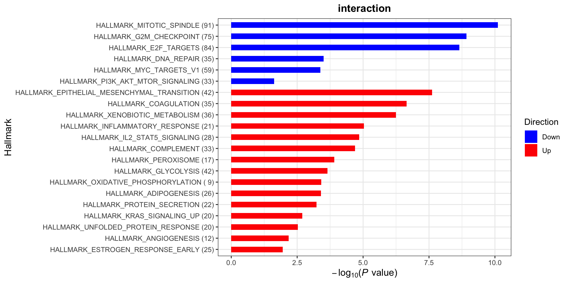
Canonical pathways
plotList$CanonicalPathway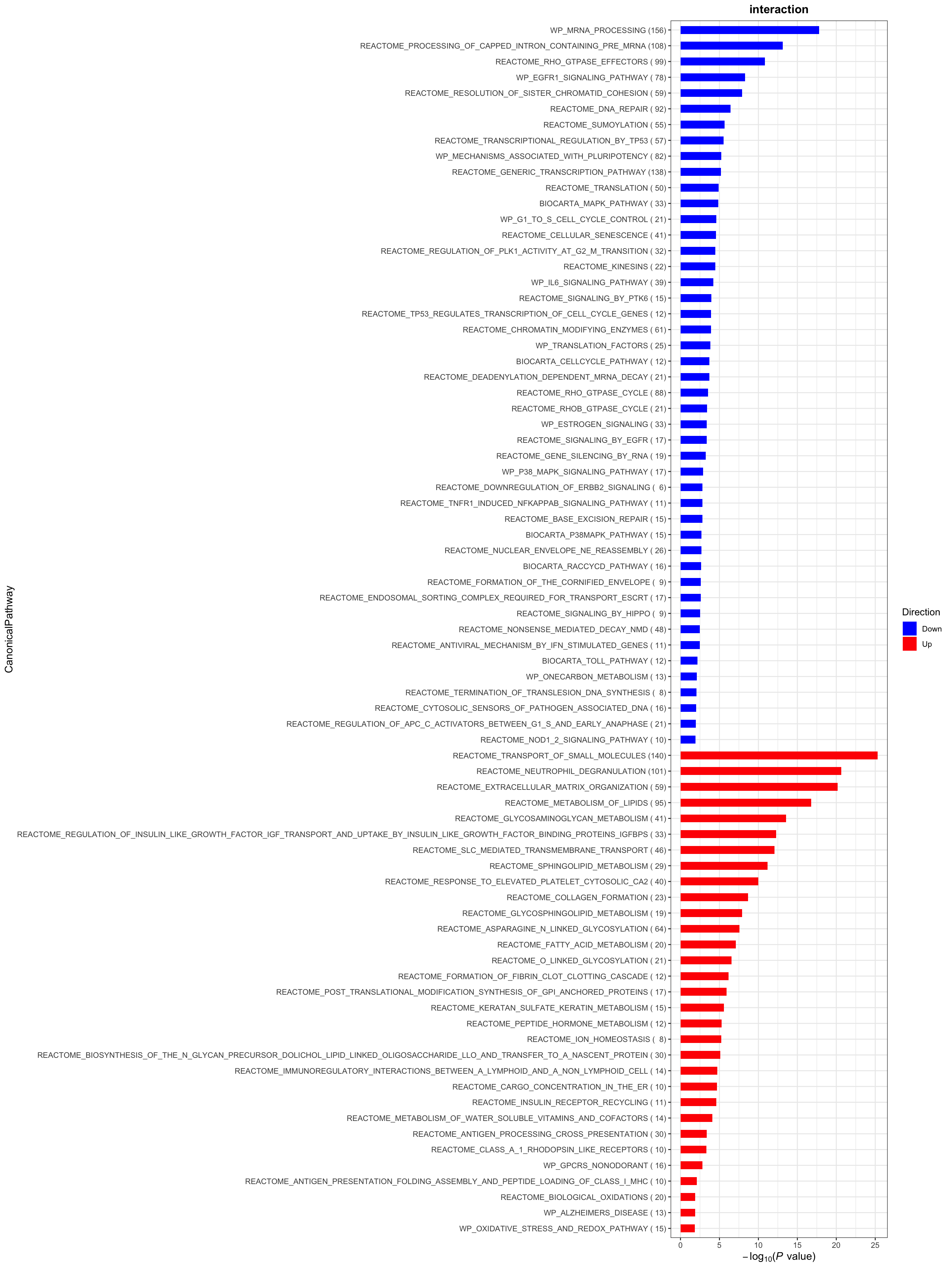
List of leading edge genes for each pathway
DT::datatable(plotList$leadingEdgeGene)writexl::write_xlsx(plotList$leadingEdgeGene, path = "../docs/enrichment_tables/prot_gsea_16combo_noMito.xlsx")Plot interesting pathways
Apoptosis
All conditions will be included, difference among cell lines will be regressed out for better visualization
plotSetHeatmap(fpeSub, filter(resTab, pval < 0.05), drugPair = "all", gmtFile = gmts$Hallmark,
setName = "HALLMARK_APOPTOSIS")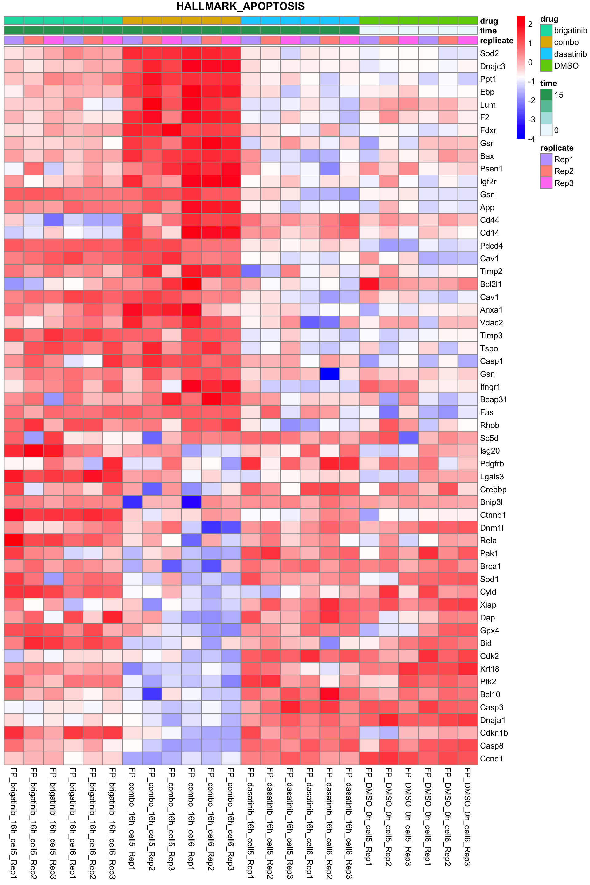
REACTOME_APOPTOTIC_CLEAVAGE_OF_CELLULAR_PROTEINS
plotSetHeatmap(fpeSub, filter(resTab, pval < 0.05), drugPair = "all", gmtFile = gmts$CanonicalPathway,
setName = "REACTOME_APOPTOTIC_CLEAVAGE_OF_CELLULAR_PROTEINS")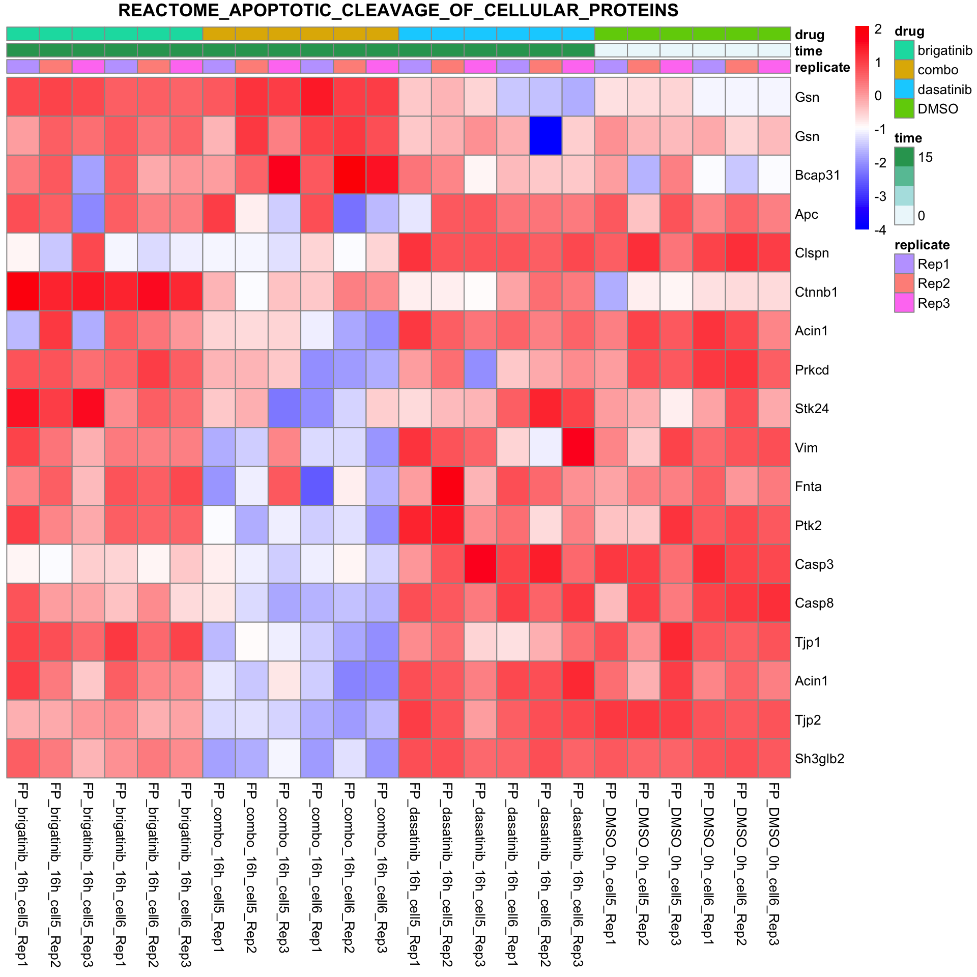
BIOCARTA_CASPASE_PATHWAY
plotSetHeatmap(fpeSub, filter(resTab, pval < 0.05), drugPair = "all", gmtFile = gmts$CanonicalPathway,
setName = "BIOCARTA_CASPASE_PATHWAY")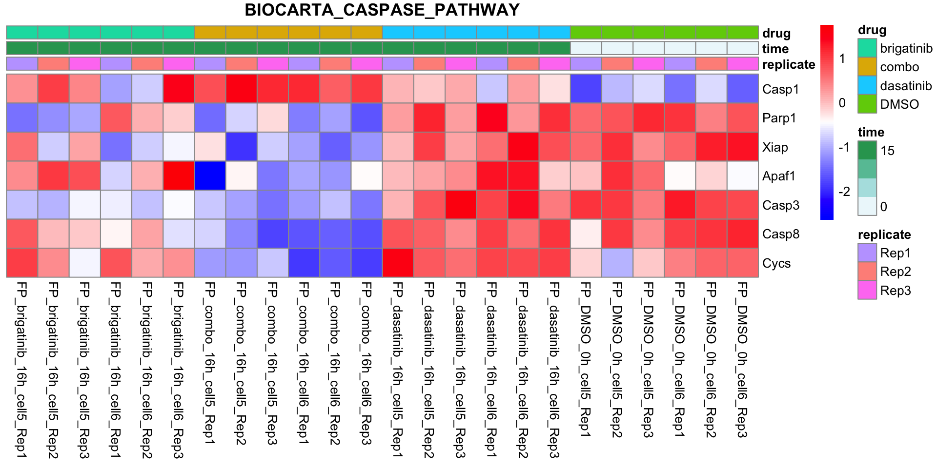
PI3K-AKT-MTOR
All conditions will be included, difference among cell lines will be regressed out for better visualization
plotSetHeatmap(fpeSub, filter(resTab, pval < 0.05), drugPair = "all", gmtFile = gmts$Hallmark,
setName = "HALLMARK_PI3K_AKT_MTOR_SIGNALING")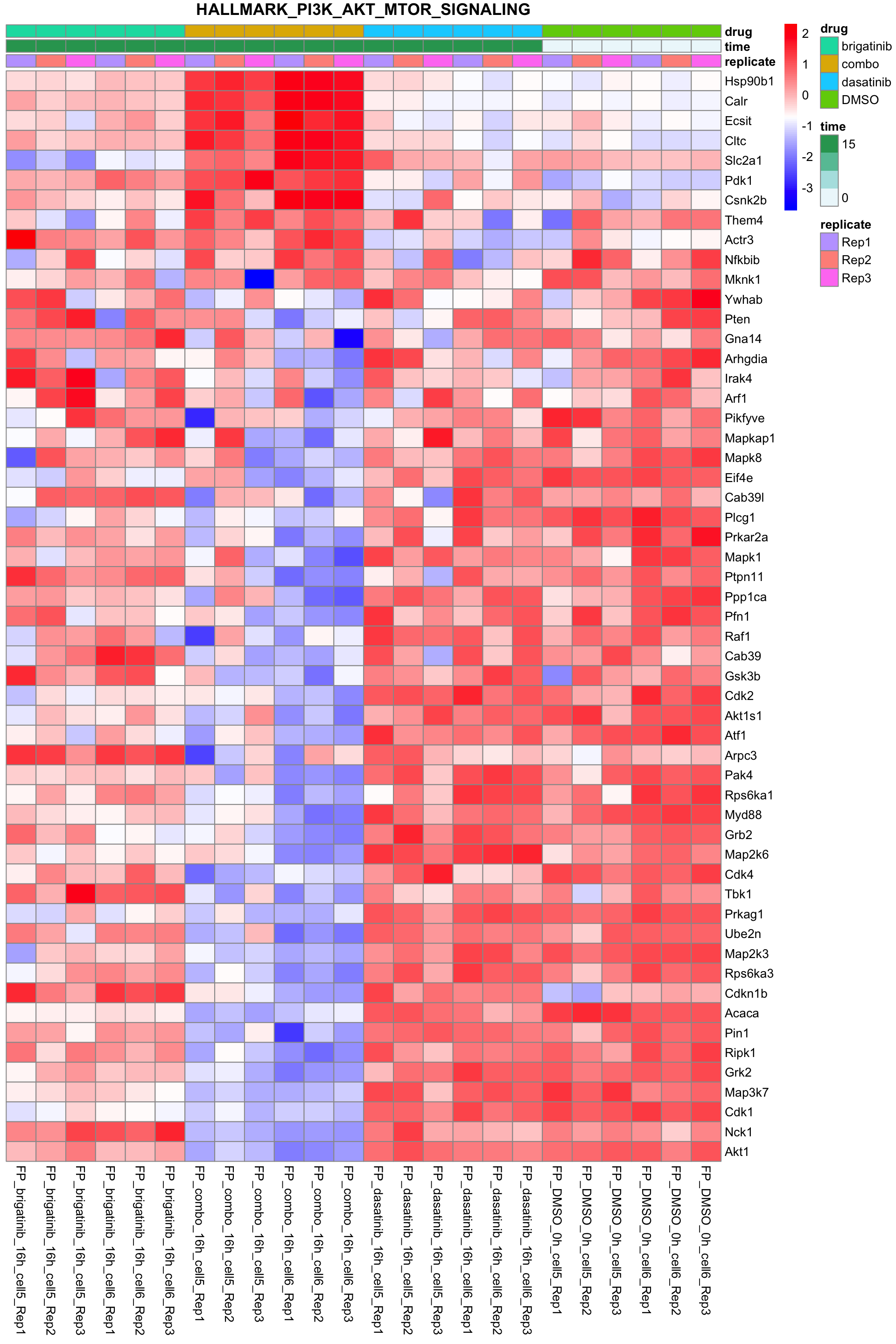
G2M_CHECKPOINT
All conditions will be included, difference among cell lines will be regressed out for better visualization
plotSetHeatmap(fpeSub, filter(resTab, pval < 0.05), drugPair = "all", gmtFile = gmts$Hallmark,
setName = "HALLMARK_G2M_CHECKPOINT")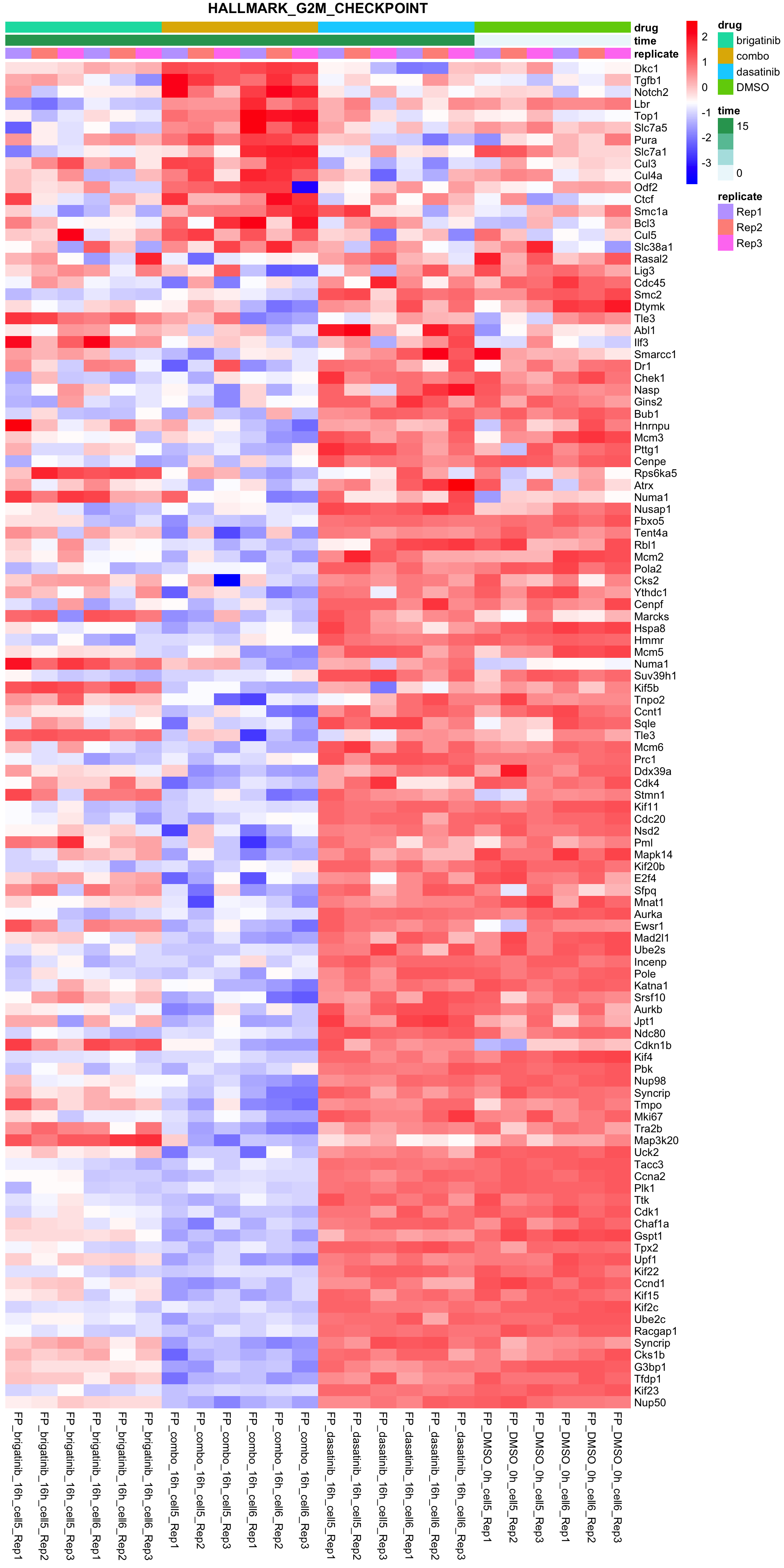
Create excel tables
Processed protein expression table
Normalized and log transformed. No imputation
seObj <- maeData[["Proteome"]][,maeData$sampleType=="FP"]
protAnno <- rowData(seObj) %>% as_tibble(rownames="id") %>%
mutate(onMitochondria = ifelse(Gene %in% mitoList,"yes","no")) %>%
select(id,Gene, onMitochondria)
protMat <- assay(seObj)
protMat <- vsn::justvsn(protMat)
protTab <- protAnno %>% left_join(as_tibble(protMat, rownames = "id"), by = "id") %>%
dplyr::select(-id)
writexl::write_xlsx(protTab, path = "../docs/protein_expression_matrix_RUN5.xlsx")Differential expression test results
output <- lapply(allResList$diffProt,
function(x) {
x <- x %>% dplyr::rename(logFoldChange = diff) %>%
dplyr::select(-name)
x
})
writexl::write_xlsx(output, path = "../docs/deProtRes_RUN5.xlsx")Heatmap plot of selected pathways
Prepare protein expression data
filterList <- list(time = c(0.17,0,16))
fpeSub <- preprocessProteome(maeData, filterList, missCut = 1, transform = "vst", normalize = TRUE)[1] "Number of proteins and samples:"
[1] 8021 42Ferroptosis
Select genes to plot
seleGene <- read_tsv("../data/ferroptosis.txt")
resTabList <- lapply(unique(seleGene$cluster2), function(x) {
geneList <- filter(seleGene, cluster2 == x)$gene
bind_rows(allResList$diffProt$time_0.17, allResList$diffProt$time_16) %>%
filter(compare %in% c("dasatinib_DMSO","brigatinib_DMSO", "combo_DMSO"),
pval <= 0.05,
toupper(symbol) %in% geneList) %>%
distinct(name, .keep_all = TRUE)
})
names(resTabList) <- unique(seleGene$cluster2)Lipid metabolism
plotProteinListHeatmap(resTabList$Lipid_metabolism, fpeSub, title = "Lipid metabolism")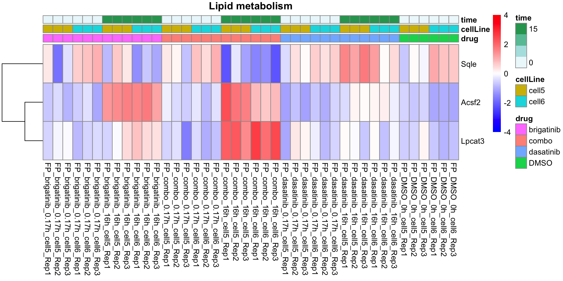
Transporters_Cys_Glutamine
plotProteinListHeatmap(resTabList$Transporters_Cys_Glutamine, fpeSub, title = "Transporters_Cys_Glutamine")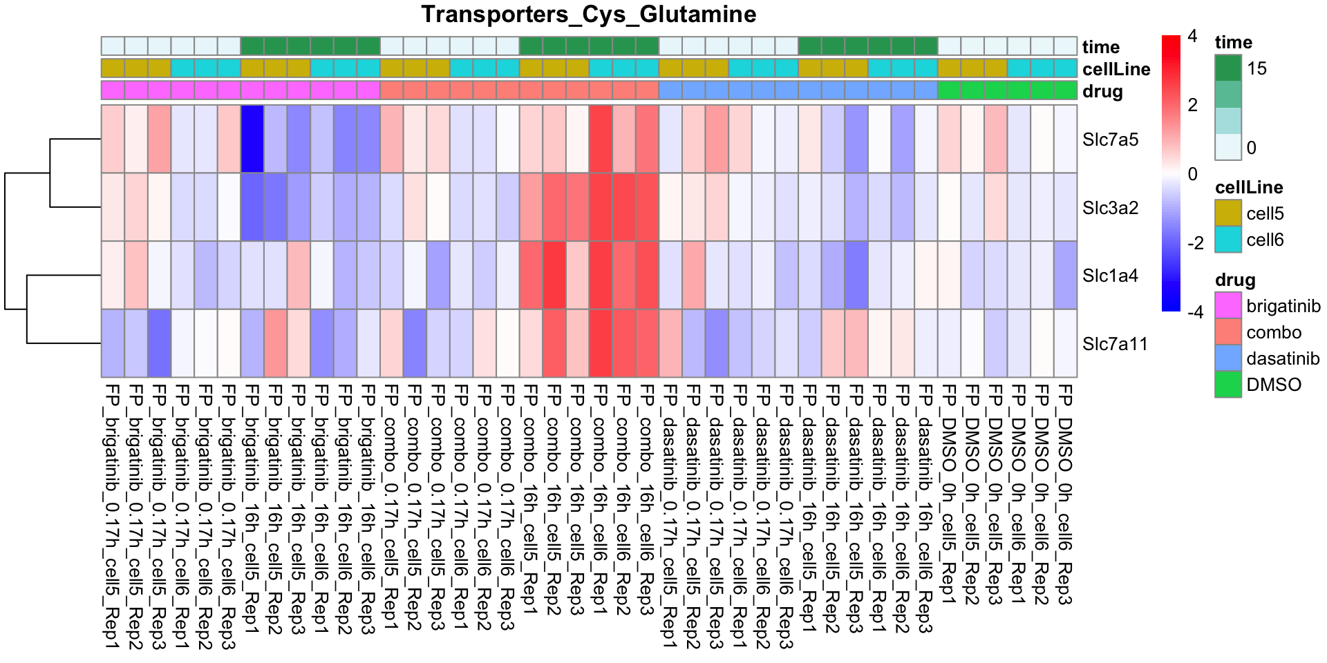
GSH_pathway
plotProteinListHeatmap(resTabList$GSH_pathway, fpeSub, title = "GSH_pathway")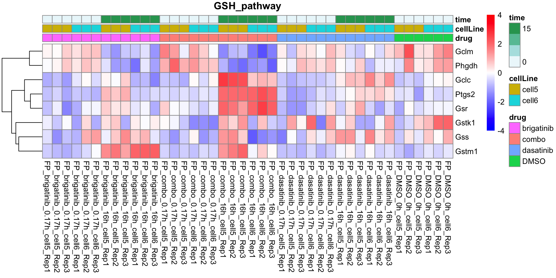
Iron_metabolsim
plotProteinListHeatmap(resTabList$Iron_metabolsim, fpeSub, title = "Iron_metabolsim")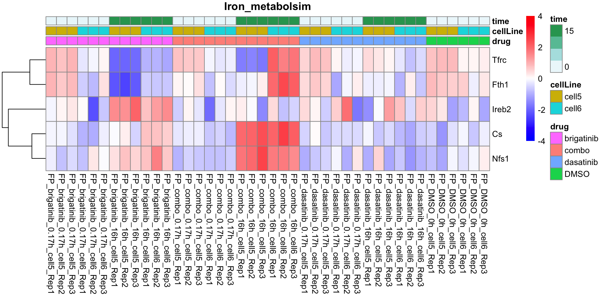
Others
plotProteinListHeatmap(resTabList$Others, fpeSub, title = "Others")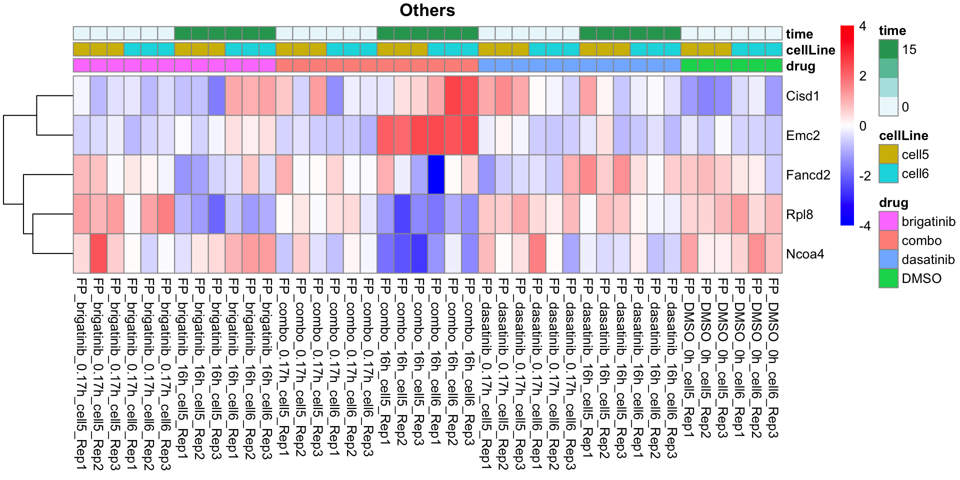
TOP
plotProteinListHeatmap(resTabList$TOP, fpeSub, title = "TOP")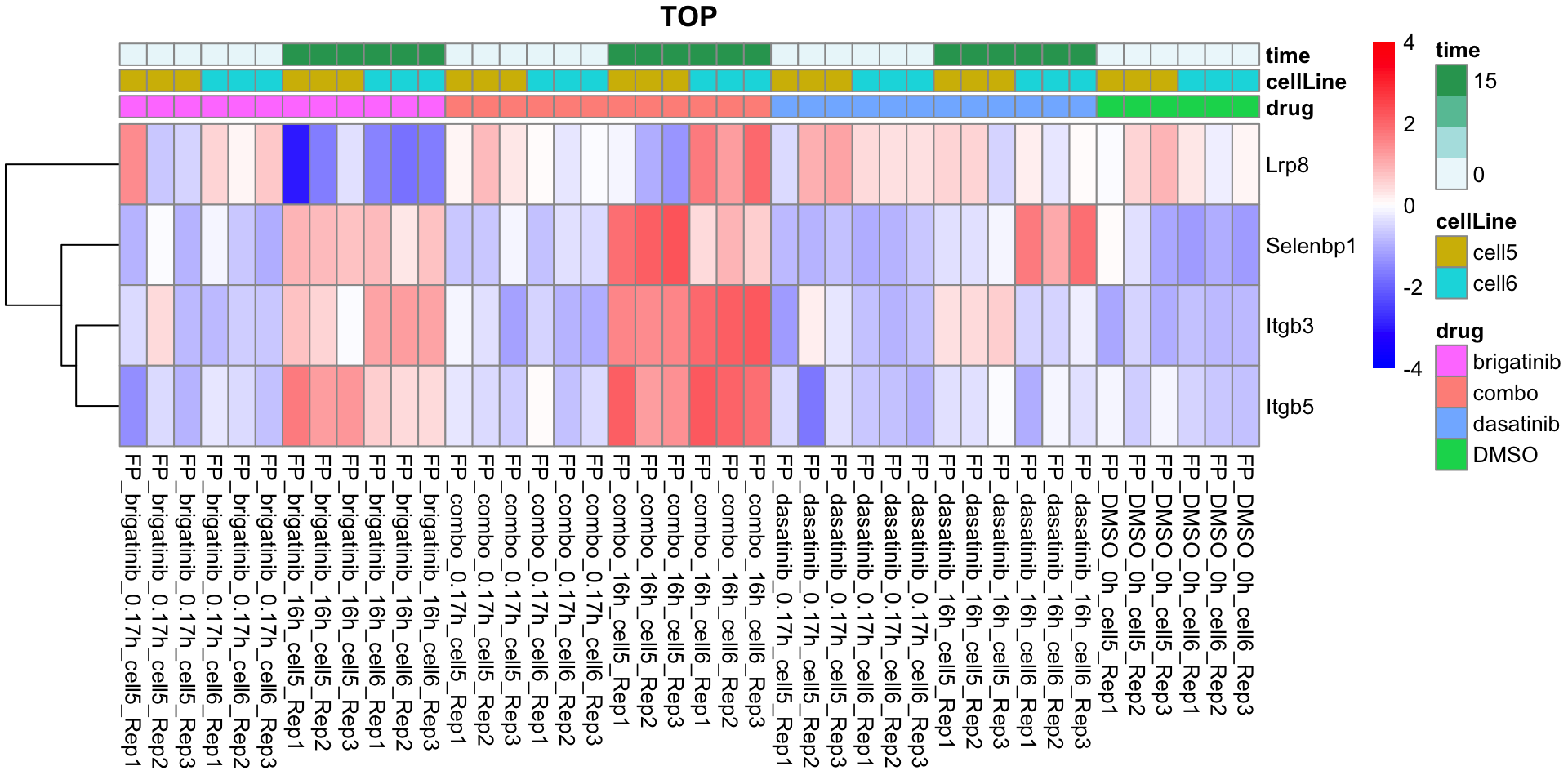
Metabolic, glycolysis, OXPHOS
Select genes to plot
seleGene <- read_csv2("../data/metabolic_glyco_oxphos.csv")
resTabList <- lapply(unique(seleGene$cluster2), function(x) {
geneList <- filter(seleGene, cluster2 == x)$gene
bind_rows(allResList$diffProt$time_0.17, allResList$diffProt$time_16) %>%
filter(compare %in% c("dasatinib_DMSO","brigatinib_DMSO", "combo_DMSO"),
pval <= 0.05,
symbol %in% geneList) %>%
distinct(name, .keep_all = TRUE)
})
names(resTabList) <- unique(seleGene$cluster2)Metabolic pathway
plotProteinListHeatmap(resTabList$Metabolic_pathway, fpeSub, title = "Metabolic_pathway")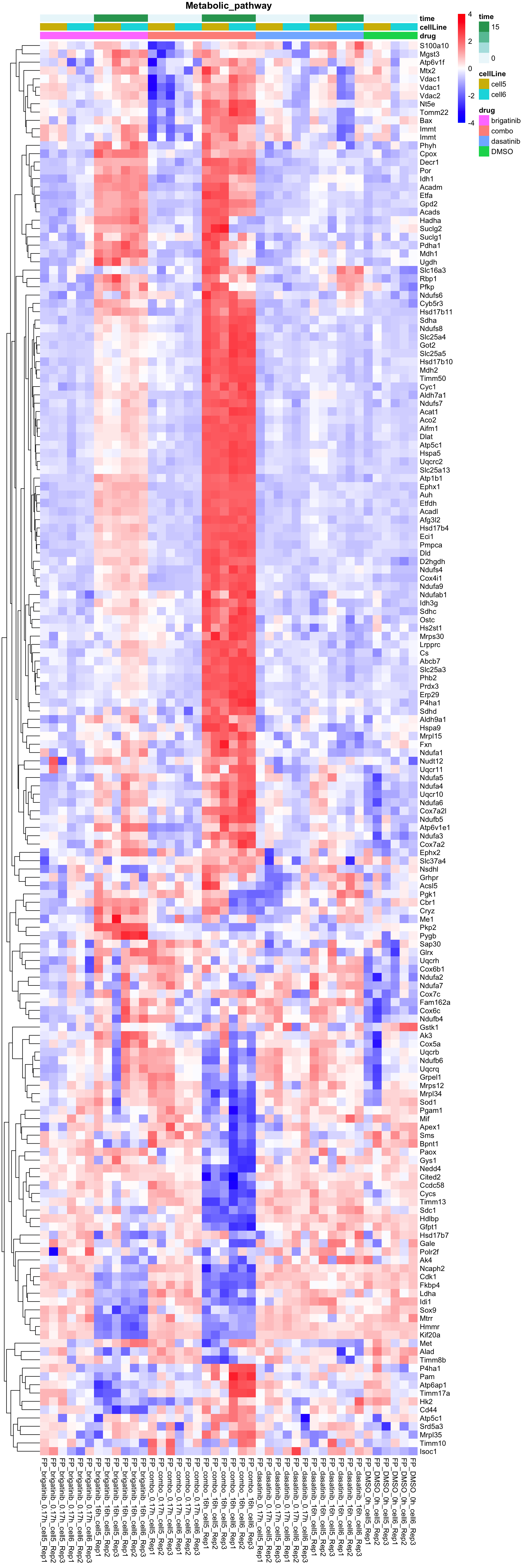
OXPHOS
plotProteinListHeatmap(resTabList$OXPHOS, fpeSub, title = "OXPHOS")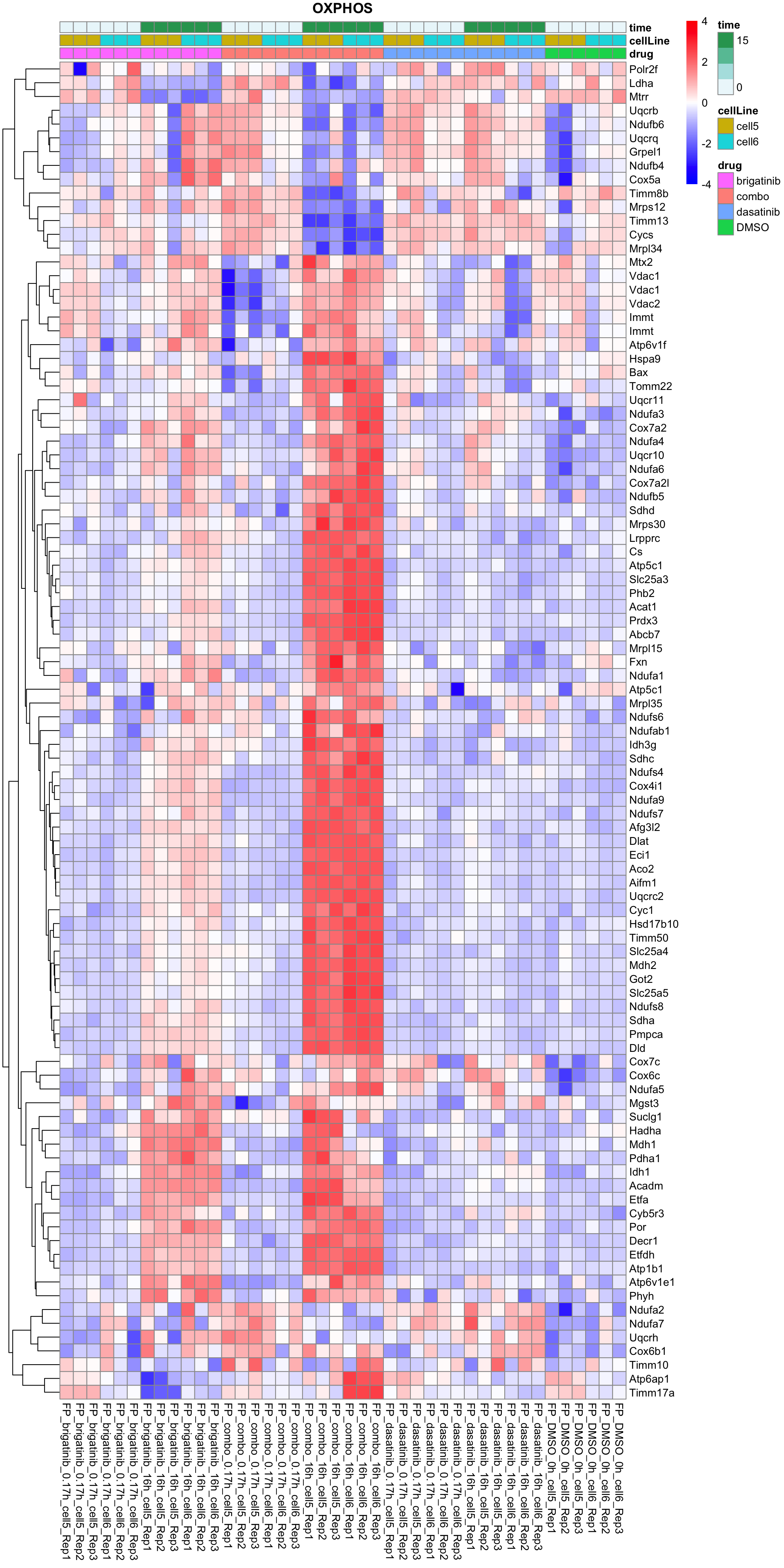
Glycolysis
plotProteinListHeatmap(resTabList$Glycolysis, fpeSub, title = "Glycolysis")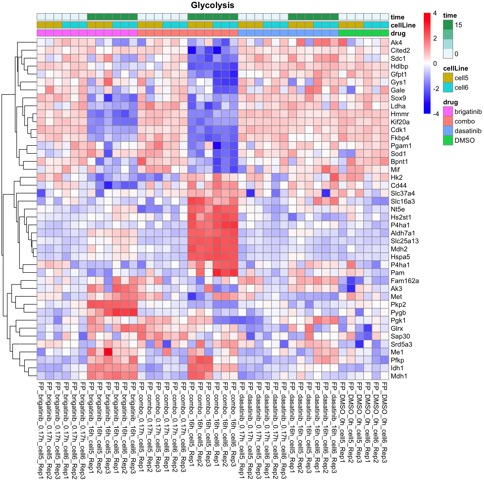
MYC pathway
Select genes to plot
seleGene <- bind_rows(tibble(gene = piano::loadGSC("../data/gmts/c2.cp.pid.v2022.1.Hs.symbols.gmt")$gsc$PID_MYC_ACTIV_PATHWAY, cluster2 = "MYC_ACTIVE_PATHWAY"),
tibble(gene = piano::loadGSC("../data/gmts/c2.cp.pid.v2022.1.Hs.symbols.gmt")$gsc$PID_MYC_REPRESS_PATHWAY, cluster2 = "PID_MYC_REPRESS_PATHWAY"))
resTabList <- lapply(unique(seleGene$cluster2), function(x) {
geneList <- filter(seleGene, cluster2 == x)$gene
bind_rows(allResList$diffProt$time_0.17, allResList$diffProt$time_16) %>%
filter(compare %in% c("dasatinib_DMSO","brigatinib_DMSO", "combo_DMSO"),
pval <= 0.05,
toupper(symbol) %in% geneList) %>%
distinct(name, .keep_all = TRUE)
})
names(resTabList) <- unique(seleGene$cluster2)MYC active pathway
plotProteinListHeatmap(resTabList$MYC_ACTIVE_PATHWAY, fpeSub, title = "MYC_ACTIVE_PATHWAY")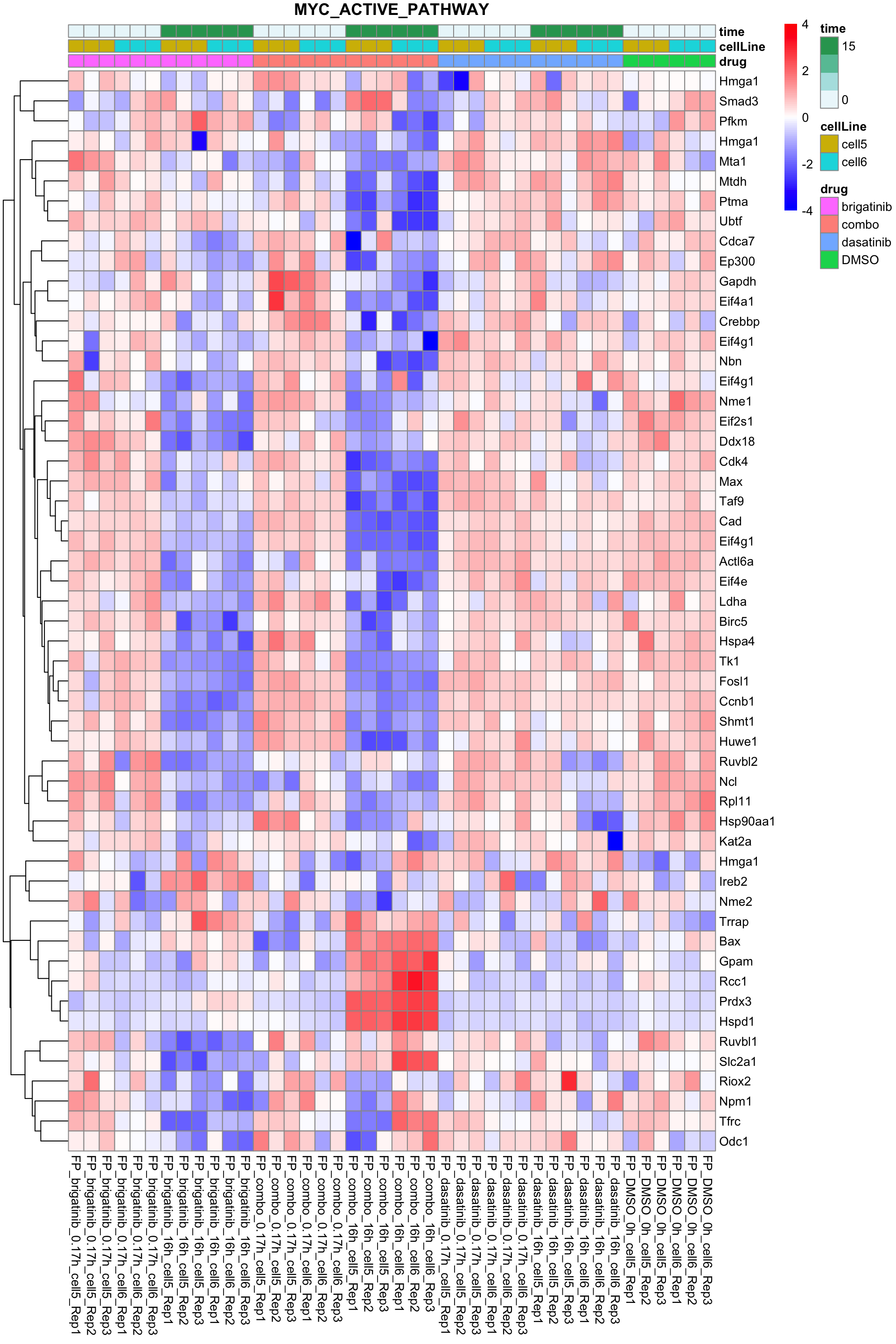
MYC repress pathway
plotProteinListHeatmap(resTabList$PID_MYC_REPRESS_PATHWAY, fpeSub, title = " MYC repress pathway")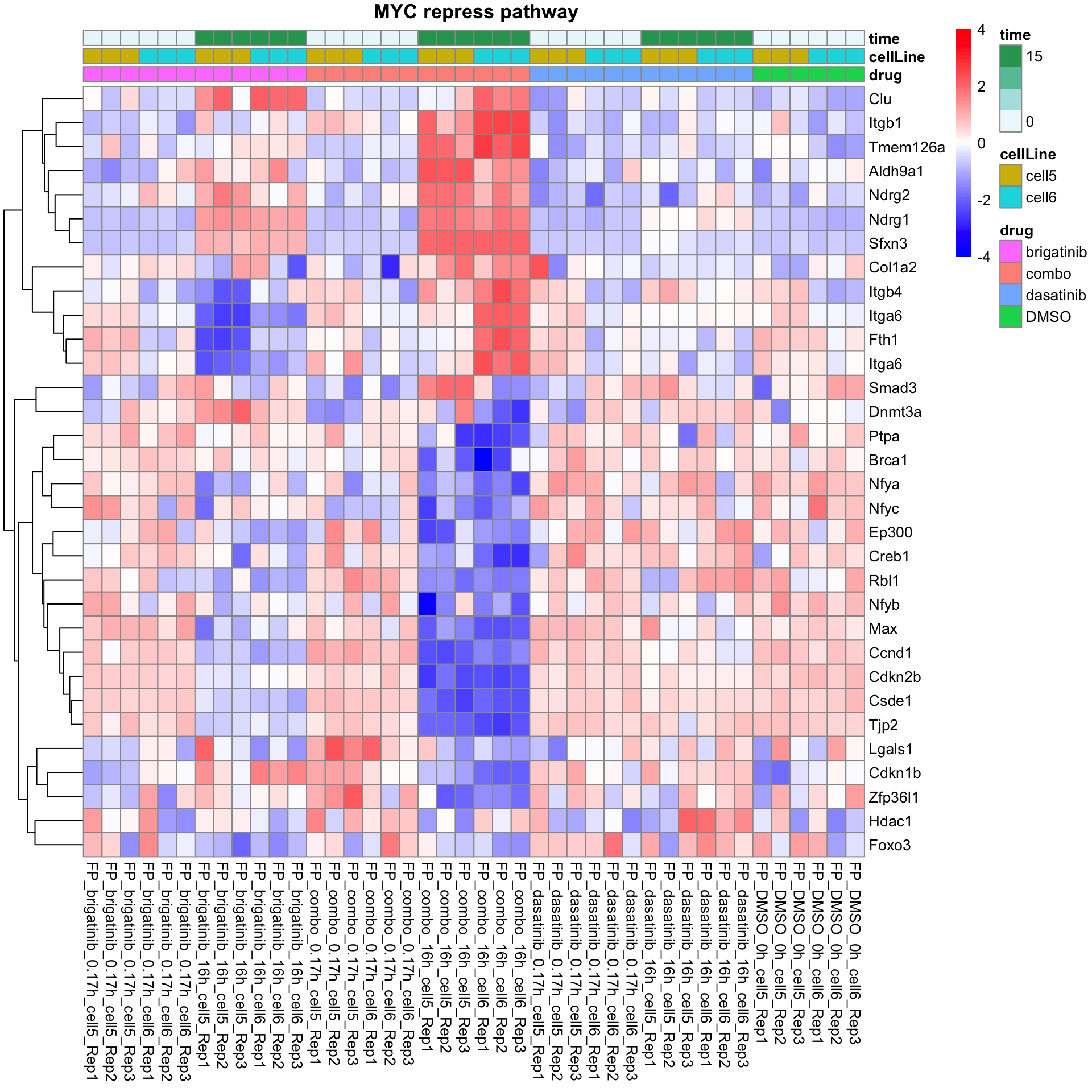
Investigate the change of Casp3 on peptide level
Load precursor peptide data (normalized by Spectronaut)
load("../output/precursorData_RUN4.RData")
preFP <- preMae[["FP"]]Get the peptides from Casp3
rowTab <- rowData(maeData[["Proteome"]])
rowTab <- rowTab %>% as_tibble() %>% filter(str_detect(Gene,"Casp3"))
rowTab# A tibble: 1 × 2
UniprotID Gene
<chr> <chr>
1 P70677 Casp3UniprotID for Casp3 is P70677
Visualize the quantification of each casp3 peptide
Get quantification for Casp3 peptides
colTab <- colData(preMae) %>% as_tibble()
pepFP <- preFP[rowData(preFP)$PG.ProteinGroups %in% "P70677",]
pepTab <- jyluMisc::sumToTidy(pepFP) %>%
group_by(colID, PEP.StrippedSequence) %>%
summarise(count = sum(count, na.rm = TRUE)) %>% ungroup() %>%
mutate(count =ifelse(count==0, NA, count)) %>%
left_join(colTab, by = c(colID = "sample")) %>%
mutate(cell = str_extract(colID,"cell.")) %>%
mutate(log2Count = log2(count))plotList <- lapply(unique(pepTab$PEP.StrippedSequence), function(pep) {
eachTab <- filter(pepTab, PEP.StrippedSequence == pep)
lineTab <- group_by(eachTab, time, drug, cell) %>%
summarise(log2Count = mean(log2Count, na.rm=TRUE))
ggplot(eachTab, aes(x=factor(time), y=log2Count)) +
geom_point(aes(col = drug)) +
geom_line(data = lineTab, aes(group = drug, col = drug)) +
facet_wrap(~cell) +
xlab("Time") + ggtitle(unique(eachTab)$PEP.StrippedSequence) +
theme_bw() +
theme(legend.position = "bottom")
})
jyluMisc::makepdf(plotList, "../docs/Casp3_peptides.pdf", ncol = 2, nrow = 4, width = 10, height = 15)Visualize the ratio between peptides abundance and the protein abundance of caps3
Use protein expression
load("../output/processedData_RUN4.RData")
caspTab <- maeData[["Proteome"]][,maeData$sampleType == "FP"]
caspTab <- caspTab[rowData(caspTab)$UniprotID == "P70677",] %>%
jyluMisc::sumToTidy() %>%
mutate(log2Val = log2(Intensity)) %>%
select(colID, log2Val)Use summarisation of peptides
caspTab <- group_by(pepTab, colID) %>%
summarise(log2Val = log2(sum(count,na.rm=TRUE)))pepTab <- mutate(pepTab, log2Protein = caspTab[match(colID, caspTab$colID),]$log2Val) %>%
mutate(logRatio = log2Count - log2Protein)plotList <- lapply(unique(pepTab$PEP.StrippedSequence), function(pep) {
eachTab <- filter(pepTab, PEP.StrippedSequence == pep)
lineTab <- group_by(eachTab, time, drug, cell) %>%
summarise(logRatio = mean(logRatio, na.rm=TRUE))
ggplot(eachTab, aes(x=factor(time), y=logRatio)) +
geom_point(aes(col = drug)) +
geom_line(data = lineTab, aes(group = drug, col = drug)) +
facet_wrap(~cell) +
xlab("Time") + ggtitle(unique(eachTab)$PEP.StrippedSequence) +
theme_bw() +
theme(legend.position = "bottom")
})
jyluMisc::makepdf(plotList, "../docs/Casp3_peptides_ratio.pdf", ncol = 2, nrow = 4, width = 10, height = 15)Visualize the quantification and ratio of large and small fragements
caspGroup <- read_tsv("../data/Casp3_group.tsv")groupTab <- mutate(pepTab, group = caspGroup[match(pepTab$PEP.StrippedSequence, caspGroup$Sequence),]$Group) %>%
filter(group %in% c("S","L", "Pro")) %>%
group_by(colID, group, time, drug, cell) %>%
summarise(count = sum(count,na.rm = TRUE)) %>%
mutate(log2Count=log2(count),
log2Protein = caspTab[match(colID, caspTab$colID),]$log2Val) %>%
mutate(logRatio = log2Count - log2Protein,
fragment = case_when(group == "L" ~ "large subunit (detected by antibody)",
group == "S" ~ "small subunit",
group == "Pro" ~ "Prodomain"))Quantification
plotList <- lapply(unique(groupTab$fragment), function(pep) {
eachTab <- filter(groupTab, fragment == pep)
lineTab <- group_by(eachTab, time, drug, cell) %>%
summarise(log2Count = mean(log2Count, na.rm=TRUE))
ggplot(eachTab, aes(x=factor(time), y=log2Count)) +
geom_point(aes(col = drug)) +
geom_line(data = lineTab, aes(group = drug, col = drug)) +
facet_wrap(~cell) +
xlab("Time") + ggtitle(unique(eachTab)$fragment) +
theme_bw() +
theme(legend.position = "bottom")
})
cowplot::plot_grid(plotlist = plotList, nrow=3)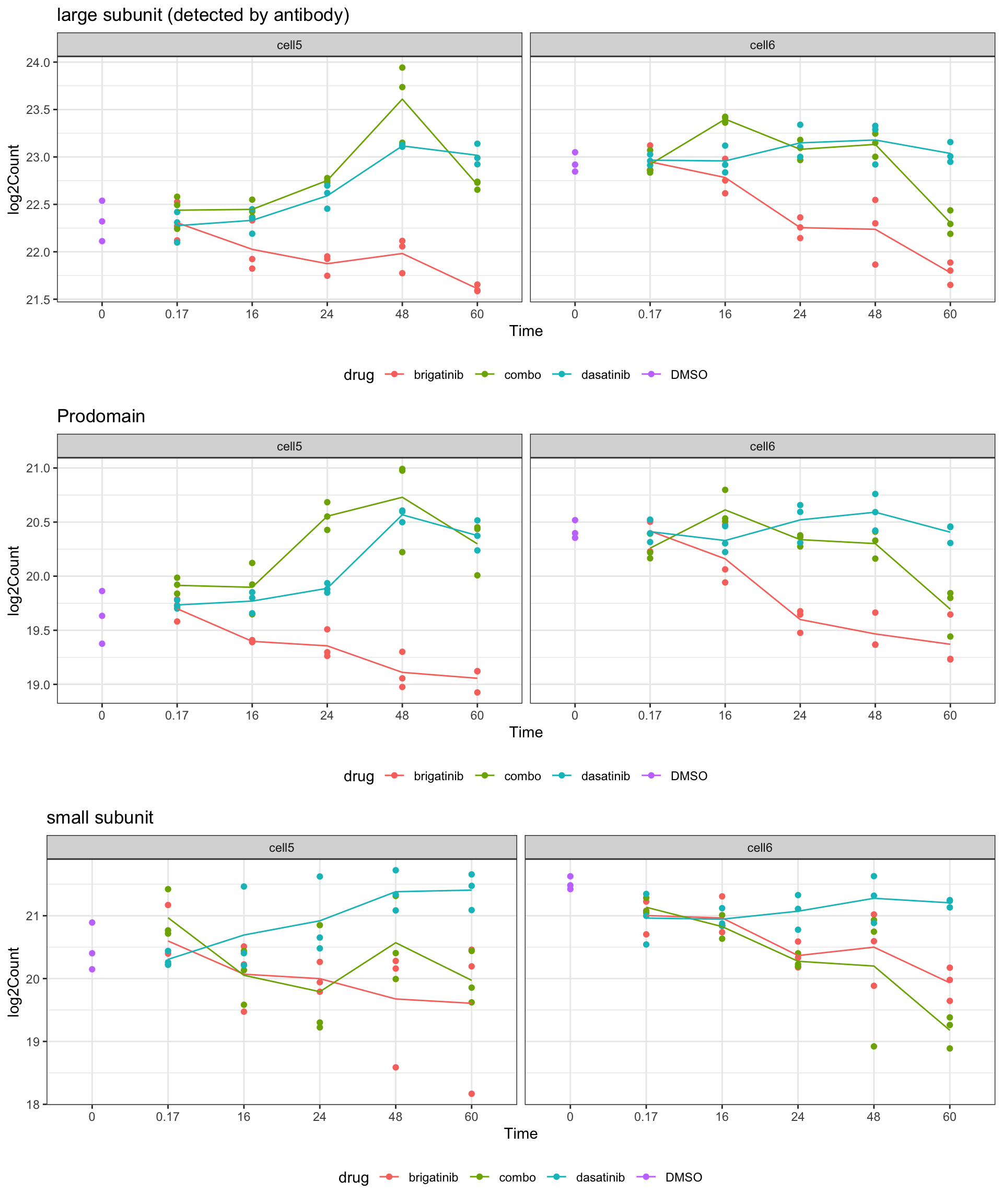
Ratio
plotList <- lapply(unique(groupTab$fragment), function(pep) {
eachTab <- filter(groupTab, fragment == pep)
lineTab <- group_by(eachTab, time, drug, cell) %>%
summarise(logRatio = mean(logRatio, na.rm=TRUE))
ggplot(eachTab, aes(x=factor(time), y=logRatio)) +
geom_point(aes(col = drug)) +
geom_line(data = lineTab, aes(group = drug, col = drug)) +
facet_wrap(~cell) +
xlab("Time") + ggtitle(unique(eachTab)$fragment) +
theme_bw() +
theme(legend.position = "bottom")
})
cowplot::plot_grid(plotlist = plotList, nrow=3)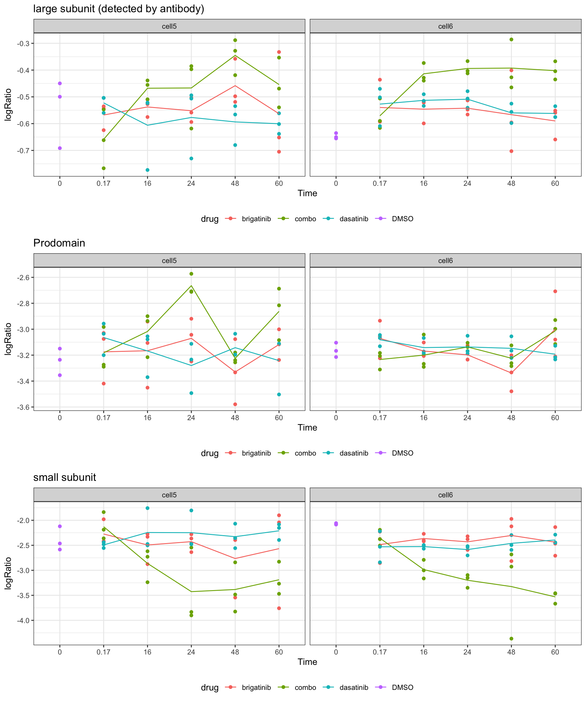
sessionInfo()R version 4.2.0 (2022-04-22)
Platform: x86_64-apple-darwin17.0 (64-bit)
Running under: macOS Big Sur/Monterey 10.16
Matrix products: default
BLAS: /Library/Frameworks/R.framework/Versions/4.2/Resources/lib/libRblas.0.dylib
LAPACK: /Library/Frameworks/R.framework/Versions/4.2/Resources/lib/libRlapack.dylib
locale:
[1] en_US.UTF-8/en_US.UTF-8/en_US.UTF-8/C/en_US.UTF-8/en_US.UTF-8
attached base packages:
[1] stats4 stats graphics grDevices utils datasets methods
[8] base
other attached packages:
[1] gridExtra_2.3 forcats_0.5.1
[3] stringr_1.4.1 dplyr_1.0.9
[5] purrr_0.3.4 readr_2.1.2
[7] tidyr_1.2.0 tibble_3.1.8
[9] ggplot2_3.4.1 tidyverse_1.3.2
[11] UpSetR_1.4.0 proDA_1.10.0
[13] MultiAssayExperiment_1.22.0 SummarizedExperiment_1.26.1
[15] Biobase_2.56.0 GenomicRanges_1.48.0
[17] GenomeInfoDb_1.32.2 IRanges_2.30.0
[19] S4Vectors_0.34.0 BiocGenerics_0.42.0
[21] MatrixGenerics_1.8.1 matrixStats_0.62.0
loaded via a namespace (and not attached):
[1] exactRankTests_0.8-35 bit64_4.0.5 knitr_1.39
[4] multcomp_1.4-19 DelayedArray_0.22.0 data.table_1.14.2
[7] KEGGREST_1.36.3 RCurl_1.98-1.7 doParallel_1.0.17
[10] generics_0.1.3 preprocessCore_1.58.0 cowplot_1.1.1
[13] TH.data_1.1-1 RSQLite_2.2.15 bit_4.0.4
[16] tzdb_0.3.0 xml2_1.3.3 lubridate_1.8.0
[19] httpuv_1.6.6 assertthat_0.2.1 gargle_1.2.0
[22] xfun_0.31 hms_1.1.1 jquerylib_0.1.4
[25] evaluate_0.15 promises_1.2.0.1 fansi_1.0.3
[28] caTools_1.18.2 dbplyr_2.2.1 readxl_1.4.0
[31] km.ci_0.5-6 igraph_1.3.4 DBI_1.1.3
[34] htmlwidgets_1.5.4 googledrive_2.0.0 ellipsis_0.3.2
[37] jyluMisc_0.1.5 crosstalk_1.2.0 ggpubr_0.4.0
[40] backports_1.4.1 annotate_1.74.0 vctrs_0.5.2
[43] imputeLCMD_2.1 abind_1.4-5 cachem_1.0.6
[46] withr_2.5.0 vroom_1.5.7 cluster_2.1.3
[49] crayon_1.5.2 drc_3.0-1 relations_0.6-12
[52] genefilter_1.78.0 edgeR_3.38.1 pkgconfig_2.0.3
[55] slam_0.1-50 labeling_0.4.2 nlme_3.1-158
[58] vipor_0.4.5 ProtGenerics_1.28.0 rlang_1.0.6
[61] lifecycle_1.0.3 sandwich_3.0-2 affyio_1.66.0
[64] modelr_0.1.8 cellranger_1.1.0 rprojroot_2.0.3
[67] Matrix_1.4-1 KMsurv_0.1-5 carData_3.0-5
[70] zoo_1.8-10 DEP_1.18.0 reprex_2.0.1
[73] beeswarm_0.4.0 GlobalOptions_0.1.2 googlesheets4_1.0.0
[76] pheatmap_1.0.12 png_0.1-7 rjson_0.2.21
[79] mzR_2.30.0 bitops_1.0-7 shinydashboard_0.7.2
[82] KernSmooth_2.23-20 visNetwork_2.1.0 Biostrings_2.64.0
[85] blob_1.2.3 workflowr_1.7.0 shape_1.4.6
[88] maxstat_0.7-25 rstatix_0.7.0 tmvtnorm_1.5
[91] ggsignif_0.6.3 scales_1.2.0 memoise_2.0.1
[94] magrittr_2.0.3 plyr_1.8.7 gplots_3.1.3
[97] zlibbioc_1.42.0 compiler_4.2.0 RColorBrewer_1.1-3
[100] plotrix_3.8-2 pcaMethods_1.88.0 clue_0.3-61
[103] cli_3.4.1 affy_1.74.0 XVector_0.36.0
[106] MASS_7.3-58 mgcv_1.8-40 tidyselect_1.1.2
[109] vsn_3.64.0 stringi_1.7.8 highr_0.9
[112] yaml_2.3.5 locfit_1.5-9.6 norm_1.0-10.0
[115] MALDIquant_1.21 survMisc_0.5.6 grid_4.2.0
[118] sass_0.4.2 fastmatch_1.1-3 tools_4.2.0
[121] parallel_4.2.0 circlize_0.4.15 rstudioapi_0.13
[124] MsCoreUtils_1.8.0 foreach_1.5.2 git2r_0.30.1
[127] farver_2.1.1 mzID_1.34.0 digest_0.6.30
[130] BiocManager_1.30.18 shiny_1.7.4 Rcpp_1.0.9
[133] car_3.1-0 broom_1.0.0 later_1.3.0
[136] writexl_1.4.0 ncdf4_1.19 httr_1.4.3
[139] survminer_0.4.9 MSnbase_2.22.0 AnnotationDbi_1.58.0
[142] ComplexHeatmap_2.12.0 colorspace_2.0-3 rvest_1.0.2
[145] XML_3.99-0.10 fs_1.5.2 splines_4.2.0
[148] gmm_1.6-6 xtable_1.8-4 jsonlite_1.8.3
[151] marray_1.74.0 R6_2.5.1 sets_1.0-21
[154] pillar_1.8.0 htmltools_0.5.4 mime_0.12
[157] glue_1.6.2 fastmap_1.1.0 DT_0.23
[160] BiocParallel_1.30.3 codetools_0.2-18 fgsea_1.22.0
[163] mvtnorm_1.1-3 utf8_1.2.2 lattice_0.20-45
[166] bslib_0.4.1 sva_3.44.0 ggbeeswarm_0.6.0
[169] gtools_3.9.3 shinyjs_2.1.0 survival_3.4-0
[172] limma_3.52.2 rmarkdown_2.14 munsell_0.5.0
[175] GetoptLong_1.0.5 GenomeInfoDbData_1.2.8 iterators_1.0.14
[178] piano_2.12.0 impute_1.70.0 haven_2.5.0
[181] gtable_0.3.0