Network analysis of drug pertubation proteomic/phosphoproteomic data
Last updated: 2023-03-13
Checks: 5 1
Knit directory:
LungCancer_SotilloLab/analysis/
This reproducible R Markdown analysis was created with workflowr (version 1.7.0). The Checks tab describes the reproducibility checks that were applied when the results were created. The Past versions tab lists the development history.
Great job! The global environment was empty. Objects defined in the global environment can affect the analysis in your R Markdown file in unknown ways. For reproduciblity it’s best to always run the code in an empty environment.
The command set.seed(20221103) was run prior to running
the code in the R Markdown file. Setting a seed ensures that any results
that rely on randomness, e.g. subsampling or permutations, are
reproducible.
Great job! Recording the operating system, R version, and package versions is critical for reproducibility.
Nice! There were no cached chunks for this analysis, so you can be confident that you successfully produced the results during this run.
Great job! Using relative paths to the files within your workflowr project makes it easier to run your code on other machines.
Tracking code development and connecting the code version to the
results is critical for reproducibility. To start using Git, open the
Terminal and type git init in your project directory.
This project is not being versioned with Git. To obtain the full
reproducibility benefits of using workflowr, please see
?wflow_start.
Load packages and dataset
Packages
#package
library(SummarizedExperiment)
library(MultiAssayExperiment)
library(tidyverse)
source("../code/utils.R")
knitr::opts_chunk$set(warning = FALSE, message = FALSE, autodep = TRUE)
Pre-processed data
load("../output/processedData_RUN5.RData")

#load saved result list
load("../output/allResList_RUN5_timeBased.RData")

#List of mitochondiral genes
mitoList <- readxl::read_xls("../data/Mouse.MitoCarta3.0.xls", sheet = 2)$Symbol

#geneset files
gmts <- list(Hallmark = "../data/gmts/mh.all.v2022.1.Mm.symbols.gmt",
             CanonicalPathway = "../data/gmts/m2.cp.v2022.1.Mm.symbols.gmt",
             TF = "../data/gmts/m3.gtrd.v2022.1.Mm.symbols.gmt",
             Kinase = "../data/gmts/Kinase_substrate.gmt",
             Kinase_noSite = "../data/gmts/Kinase_substrate_noSite.gmt")
Kinase-target network
10 mins
Construct network
Differential results
resList <- allResList$diffRatio$time_0.17 %>%
  filter(compare %in% c("combo_DMSO","brigatinib_DMSO","dasatinib_DMSO"))
Kinase-target network structure from database
kinNet <- piano::loadGSC(gmts$Kinase)$gsc
kinNet <- lapply(names(kinNet), function(x) {
  tibble(Kinase = x,
         Target = kinNet[[x]])
}) %>% bind_rows()
netTab <- left_join(resList, kinNet, by = c(site = "Target")) %>%
filter(!is.na(Kinase)) %>%
dplyr::rename(from = Kinase, to = site)Created edge and vertex tables
edgeTab <- filter(netTab, pval <= 0.05) %>%
  select(from, to, pval, adj_pval, diff, compare) %>%
  mutate(compare = str_remove(compare,"_DMSO"),
         logP = -log10(pval),
         regulate = ifelse(diff >0 ,"up","down"))
nodeTab <- select(edgeTab, from, to) %>%
  pivot_longer(c(from, to), names_to = "type",values_to = "name") %>%
  distinct(name, .keep_all = TRUE) %>%
  select(name, type) %>%
  mutate(type = ifelse(type == "from", "Kinase", "Substrate"))
Visualization in network
library(tidygraph)
library(ggraph)
tNet <- tbl_graph(nodes = nodeTab, edges = edgeTab, directed = TRUE)


phosNet <- ggraph(tNet, layout = "kk") +
  geom_edge_fan(aes(color = compare, linetype = regulate, width = logP)) +
  geom_node_point(aes(color = type, shape = type), size=6) +
  geom_node_text(aes(label = name), repel = TRUE, size=6) +
  scale_edge_linetype_manual(values = c(down = "dotted", up = "solid"))+
  scale_color_manual(values = c(Kinase = "cyan", Substrate = "salmon")) +
  scale_edge_color_manual(values = c(combo = "darkblue", dasatinib = "green", brigatinib = "pink")) +
  theme_graph(base_family = "sans") + theme(legend.position = "bottom")
phosNet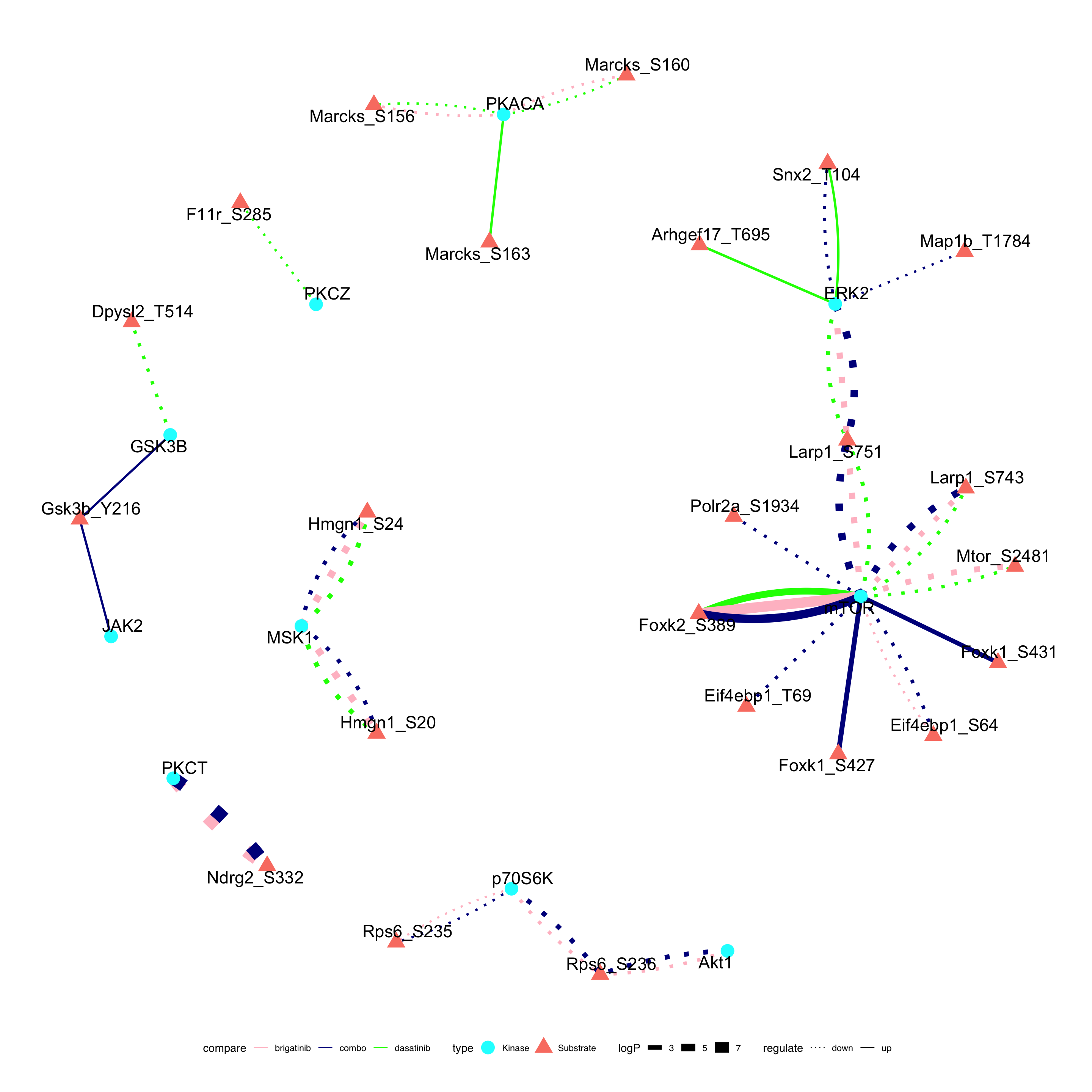
16 hours
Construct network
Differential results
resList <- allResList$diffRatio$time_16 %>%
  filter(compare %in% c("combo_DMSO","brigatinib_DMSO","dasatinib_DMSO"))
Kinase-target network structure from database
kinNet <- piano::loadGSC(gmts$Kinase)$gsc
kinNet <- lapply(names(kinNet), function(x) {
  tibble(Kinase = x,
         Target = kinNet[[x]])
}) %>% bind_rows()
netTab <- left_join(resList, kinNet, by = c(site = "Target")) %>%
filter(!is.na(Kinase)) %>%
dplyr::rename(from = Kinase, to = site)Created edge and vertex tables
edgeTab <- filter(netTab, pval <= 0.05) %>%
  select(from, to, pval, adj_pval, diff, compare) %>%
  mutate(compare = str_remove(compare,"_DMSO"),
         logP = -log10(pval),
         regulate = ifelse(diff >0 ,"up","down"))
nodeTab <- select(edgeTab, from, to) %>%
  pivot_longer(c(from, to), names_to = "type",values_to = "name") %>%
  distinct(name, .keep_all = TRUE) %>%
  select(name, type) %>%
  mutate(type = ifelse(type == "from", "Kinase", "Substrate"))
Visualization in network
library(tidygraph)
library(ggraph)
tNet <- tbl_graph(nodes = nodeTab, edges = edgeTab, directed = TRUE)


phosNet <- ggraph(tNet, layout = "kk") +
  geom_edge_fan(aes(color = compare, linetype = regulate, width =logP)) +
  geom_node_point(aes(color = type, shape = type), size=6) +
  geom_node_text(aes(label = name), repel = TRUE, size=6) +
  scale_edge_linetype_manual(values = c(down = "dotted", up = "solid"))+
  scale_color_manual(values = c(Kinase = "cyan", Substrate = "salmon")) +
  scale_edge_color_manual(values = c(combo = "darkblue", dasatinib = "green", brigatinib = "pink")) +
  theme_graph(base_family = "sans") + theme(legend.position = "bottom")
phosNet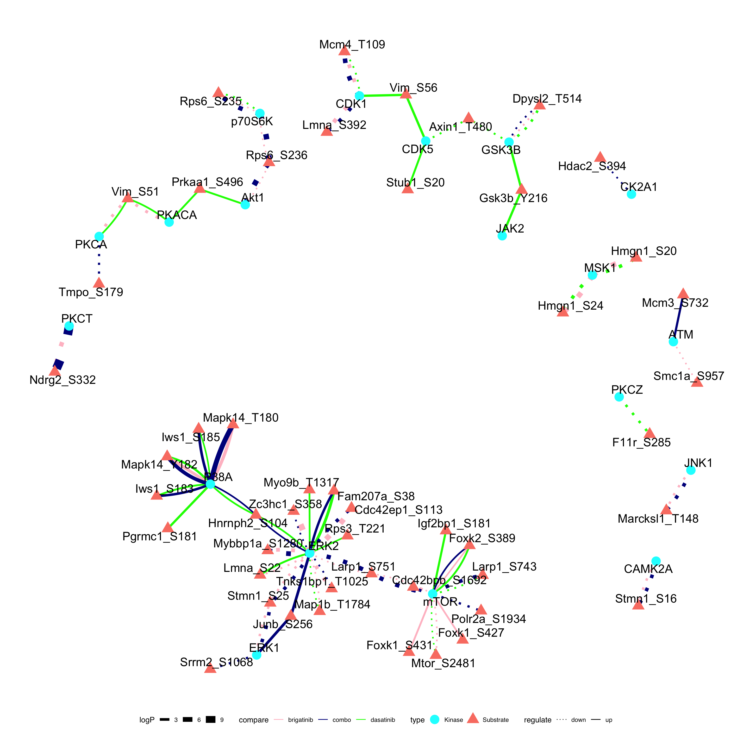
STRING network construction
10 min, comparing drugs to DMSO
Prepare data
resList <- allResList$diffProt$time_0.17 %>%
  filter(compare %in% c("combo_DMSO","brigatinib_DMSO","dasatinib_DMSO")) %>%
  filter(pval < 0.01)
Construct STRING network
library(STRINGdb)
string_db <- STRINGdb$new(version = "11.5", species = 10090, network_type="physical", input_directory="../data/STRING/")
WARNING: Score threshold is not specified. We will be using medium stringency cut-off of 400.Up-regulated
subList <- filter(resList, diff>0)
strNet <- string_db$map(data.frame(subList), "symbol", removeUnmappedRows = TRUE)
Warning: we couldn't map to STRING 0% of your identifiersedgeTab <- string_db$get_interactions(strNet$STRING_id) %>%
distinct(from, to)
nodeTab <- subList %>%
mutate(name = strNet[match(toupper(symbol), strNet$symbol),]$STRING_id) %>%
filter(!is.na(name), !is.na(symbol)) %>%
distinct(name, symbol, compare) %>%
mutate(compare = str_remove(compare,"_DMSO"))
nodeGroup <- nodeTab %>% select(name, compare) %>%
mutate(fillVal =compare) %>%
mutate(fillVal = ifelse(fillVal == "dasatinib","dasa",
ifelse(fillVal == "brigatinib","brig","combo"))) %>%
distinct(name, compare, fillVal) %>%
pivot_wider(names_from = compare, values_from = fillVal) %>%
#mutate(across(everything(),replace_na,"")) %>%
mutate(groupType = paste0(dasatinib,"_",brigatinib,"_",combo)) %>%
mutate(groupType = str_remove_all(groupType,"NA_|_NA")) %>%
mutate(groupType = ifelse(groupType == "dasa_brig_combo","all",groupType))
nodeTab <- mutate(nodeTab,
nodeType = nodeGroup[match(name, nodeGroup$name),]$groupType) %>%
distinct(name, nodeType, symbol)
#remove isolated nodes
edgeTab <- filter(edgeTab, from %in% nodeTab$name, to %in% nodeTab$name)
nodeTab <- filter(nodeTab, name %in% edgeTab$from | name %in% edgeTab$to)upNet <- tbl_graph(nodes = nodeTab, edges = edgeTab, directed = FALSE)
ggraph(upNet, layout = "igraph", algorithm = "nicely") +
geom_edge_link() +
geom_node_point(aes(color = nodeType), size=6) +
geom_node_text(aes(label = symbol), size=4) +
theme_graph(base_family = "sans") + theme(legend.position = "bottom") 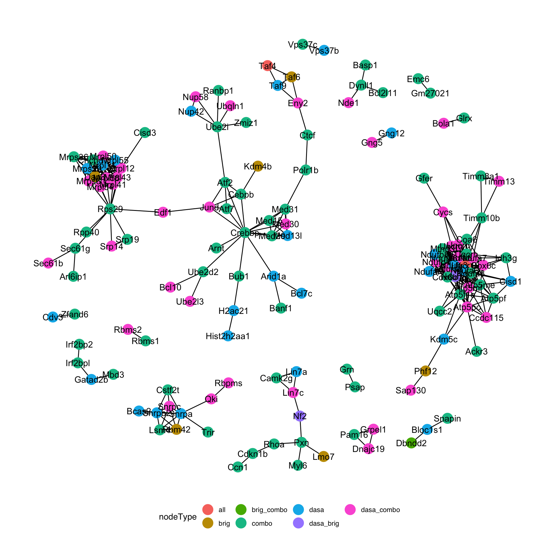
Down-regulated
subList <- filter(resList, diff<0)
strNet <- string_db$map(data.frame(subList), "symbol", removeUnmappedRows = TRUE)
Warning: we couldn't map to STRING 1% of your identifiersedgeTab <- string_db$get_interactions(strNet$STRING_id) %>%
distinct(from, to)
nodeTab <- subList %>%
mutate(name = strNet[match(toupper(symbol), strNet$symbol),]$STRING_id) %>%
filter(!is.na(name)) %>%
select(name, symbol, compare) %>%
mutate(compare = str_remove(compare,"_DMSO"))
nodeGroup <- nodeTab %>% select(name, compare) %>%
mutate(fillVal =compare) %>%
mutate(fillVal = ifelse(fillVal == "dasatinib","dasa",
ifelse(fillVal == "brigatinib","brig","combo"))) %>%
distinct(name, compare, fillVal) %>%
pivot_wider(names_from = compare, values_from = fillVal) %>%
#mutate(across(everything(),replace_na,"")) %>%
mutate(groupType = paste0(dasatinib,"_",brigatinib,"_",combo)) %>%
mutate(groupType = str_remove_all(groupType,"NA_|_NA")) %>%
mutate(groupType = ifelse(groupType == "dasa_brig_combo","all",groupType))
nodeTab <- mutate(nodeTab,
nodeType = nodeGroup[match(name, nodeGroup$name),]$groupType) %>%
distinct(name, nodeType, symbol)
#remove isolated nodes
#remove isolated nodes
edgeTab <- filter(edgeTab, from %in% nodeTab$name, to %in% nodeTab$name)
nodeTab <- filter(nodeTab, name %in% edgeTab$from | name %in% edgeTab$to)downNet <- tbl_graph(nodes = nodeTab, edges = edgeTab)
ggraph(downNet, layout = "igraph", algorithm = "nicely") +
geom_edge_link() +
geom_node_point(aes(color = nodeType), size=6) +
geom_node_text(aes(label = symbol), size=4) +
theme_graph(base_family = "sans") + theme(legend.position = "bottom") 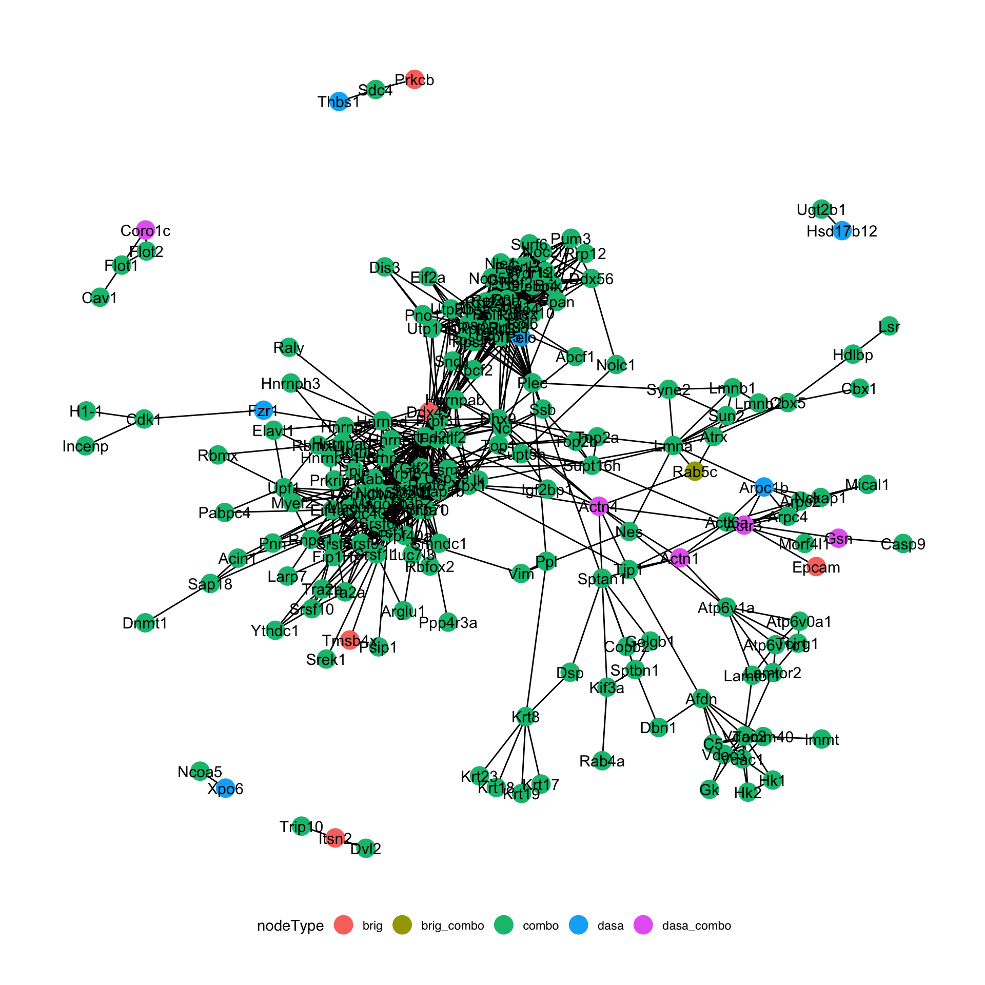
sessionInfo()R version 4.2.0 (2022-04-22)
Platform: x86_64-apple-darwin17.0 (64-bit)
Running under: macOS Big Sur/Monterey 10.16
Matrix products: default
BLAS: /Library/Frameworks/R.framework/Versions/4.2/Resources/lib/libRblas.0.dylib
LAPACK: /Library/Frameworks/R.framework/Versions/4.2/Resources/lib/libRlapack.dylib
locale:
[1] en_US.UTF-8/en_US.UTF-8/en_US.UTF-8/C/en_US.UTF-8/en_US.UTF-8
attached base packages:
[1] stats4 stats graphics grDevices utils datasets methods
[8] base
other attached packages:
[1] STRINGdb_2.8.4 ggraph_2.0.5
[3] tidygraph_1.2.1 forcats_0.5.1
[5] stringr_1.4.1 dplyr_1.0.9
[7] purrr_0.3.4 readr_2.1.2
[9] tidyr_1.2.0 tibble_3.1.8
[11] ggplot2_3.4.1 tidyverse_1.3.2
[13] MultiAssayExperiment_1.22.0 SummarizedExperiment_1.26.1
[15] Biobase_2.56.0 GenomicRanges_1.48.0
[17] GenomeInfoDb_1.32.2 IRanges_2.30.0
[19] S4Vectors_0.34.0 BiocGenerics_0.42.0
[21] MatrixGenerics_1.8.1 matrixStats_0.62.0
loaded via a namespace (and not attached):
[1] readxl_1.4.0 backports_1.4.1 fastmatch_1.1-3
[4] workflowr_1.7.0 plyr_1.8.7 igraph_1.3.4
[7] shinydashboard_0.7.2 BiocParallel_1.30.3 digest_0.6.30
[10] htmltools_0.5.4 viridis_0.6.2 fansi_1.0.3
[13] memoise_2.0.1 magrittr_2.0.3 googlesheets4_1.0.0
[16] cluster_2.1.3 tzdb_0.3.0 limma_3.52.2
[19] graphlayouts_0.8.0 modelr_0.1.8 piano_2.12.0
[22] colorspace_2.0-3 blob_1.2.3 rvest_1.0.2
[25] ggrepel_0.9.1 haven_2.5.0 xfun_0.31
[28] crayon_1.5.2 RCurl_1.98-1.7 jsonlite_1.8.3
[31] glue_1.6.2 hash_2.2.6.2 polyclip_1.10-0
[34] gtable_0.3.0 gargle_1.2.0 zlibbioc_1.42.0
[37] XVector_0.36.0 DelayedArray_0.22.0 scales_1.2.0
[40] DBI_1.1.3 relations_0.6-12 Rcpp_1.0.9
[43] plotrix_3.8-2 viridisLite_0.4.0 xtable_1.8-4
[46] bit_4.0.4 sqldf_0.4-11 DT_0.23
[49] htmlwidgets_1.5.4 httr_1.4.3 fgsea_1.22.0
[52] gplots_3.1.3 RColorBrewer_1.1-3 ellipsis_0.3.2
[55] pkgconfig_2.0.3 farver_2.1.1 sass_0.4.2
[58] dbplyr_2.2.1 utf8_1.2.2 tidyselect_1.1.2
[61] labeling_0.4.2 rlang_1.0.6 later_1.3.0
[64] munsell_0.5.0 cellranger_1.1.0 tools_4.2.0
[67] visNetwork_2.1.0 cachem_1.0.6 cli_3.4.1
[70] gsubfn_0.7 RSQLite_2.2.15 generics_0.1.3
[73] broom_1.0.0 evaluate_0.15 fastmap_1.1.0
[76] yaml_2.3.5 bit64_4.0.5 knitr_1.39
[79] fs_1.5.2 caTools_1.18.2 mime_0.12
[82] slam_0.1-50 xml2_1.3.3 compiler_4.2.0
[85] rstudioapi_0.13 png_0.1-7 marray_1.74.0
[88] reprex_2.0.1 tweenr_1.0.2 bslib_0.4.1
[91] stringi_1.7.8 highr_0.9 lattice_0.20-45
[94] Matrix_1.4-1 shinyjs_2.1.0 vctrs_0.5.2
[97] pillar_1.8.0 lifecycle_1.0.3 jquerylib_0.1.4
[100] data.table_1.14.2 bitops_1.0-7 httpuv_1.6.6
[103] R6_2.5.1 promises_1.2.0.1 KernSmooth_2.23-20
[106] gridExtra_2.3 codetools_0.2-18 MASS_7.3-58
[109] gtools_3.9.3 assertthat_0.2.1 chron_2.3-58
[112] proto_1.0.0 rprojroot_2.0.3 withr_2.5.0
[115] GenomeInfoDbData_1.2.8 parallel_4.2.0 hms_1.1.1
[118] grid_4.2.0 rmarkdown_2.14 googledrive_2.0.0
[121] git2r_0.30.1 sets_1.0-21 ggforce_0.3.3
[124] shiny_1.7.4 lubridate_1.8.0