Analysis of the V1 V3 mTDCs proteomic data for the manuscript
Last updated: 2023-05-27
Checks: 5 1
Knit directory:
LungCancer_SotilloLab/analysis/
This reproducible R Markdown analysis was created with workflowr (version 1.7.0). The Checks tab describes the reproducibility checks that were applied when the results were created. The Past versions tab lists the development history.
Great job! The global environment was empty. Objects defined in the global environment can affect the analysis in your R Markdown file in unknown ways. For reproduciblity it’s best to always run the code in an empty environment.
The command set.seed(20221103) was run prior to running
the code in the R Markdown file. Setting a seed ensures that any results
that rely on randomness, e.g. subsampling or permutations, are
reproducible.
Great job! Recording the operating system, R version, and package versions is critical for reproducibility.
Nice! There were no cached chunks for this analysis, so you can be confident that you successfully produced the results during this run.
Great job! Using relative paths to the files within your workflowr project makes it easier to run your code on other machines.
Tracking code development and connecting the code version to the
results is critical for reproducibility. To start using Git, open the
Terminal and type git init in your project directory.
This project is not being versioned with Git. To obtain the full
reproducibility benefits of using workflowr, please see
?wflow_start.
Load packages and dataset
#package
library(DEP)
library(SummarizedExperiment)
library(MultiAssayExperiment)
library(proDA)
library(tidyverse)
source("../code/utils.R")
knitr::opts_chunk$set(warning = FALSE, message = FALSE)

#dataset
load("../output/fpe_V1V2_DDA.RData")
Figure 1: Differentially expressed proteins between V1 and V3 mTDCs
Data preprocesing
Subset dataset
fpeSub <- fpe[,fpe$treatment == "dmso"]

keepVal <- rowSums(is.na(assay(fpeSub)))/ncol(fpeSub) <= 0.5
fpeSub <- fpeSub[keepVal,]

assay(fpeSub) <- log2(assay(fpeSub))
Imputation for PCA
imp <- DEP::impute(fpeSub, "bpca")
assays(fpeSub)[["imputed"]] <- assay(imp)
PCA plot (Supplementary Figure 1D)
v3Color <- "#DC7970"
v1Color <- "#EAEAEA"

exprMat <- assays(fpeSub)[["imputed"]]
smpAnno <- colData(fpeSub) %>% as_tibble()
pcRes <- prcomp(t(exprMat))
varExp <- pcRes$sdev^2/sum(pcRes$sdev^2)*100

pcTab <- pcRes$x[,1:2] %>%
    as_tibble(rownames = "sampleID") %>%
    left_join(smpAnno)

ggplot(pcTab, aes(x=PC1, y=PC2)) +
  geom_point(aes(fill = EA_variant), shape = 21, size=5) +
  scale_fill_manual(values = c(V1 = v1Color, V3= v3Color), name = bquote(italic("EA")~"variant"))+
  scale_x_continuous(limits = c(-18,18), breaks = seq(-15,15,5)) +
  scale_y_continuous(limits = c(-18,18), breaks = seq(-15,15,5)) +
  xlab(sprintf("PC1 (%1.1f%%)",varExp[1])) +
  ylab(sprintf("PC2 (%1.1f%%)",varExp[2])) +
  theme_bw() +
  theme(panel.border = element_blank(),
        legend.position = c(0.2,0.8),
        legend.box.background  = element_rect(),
        axis.title = element_text(size=15),
        axis.text = element_text(size=15))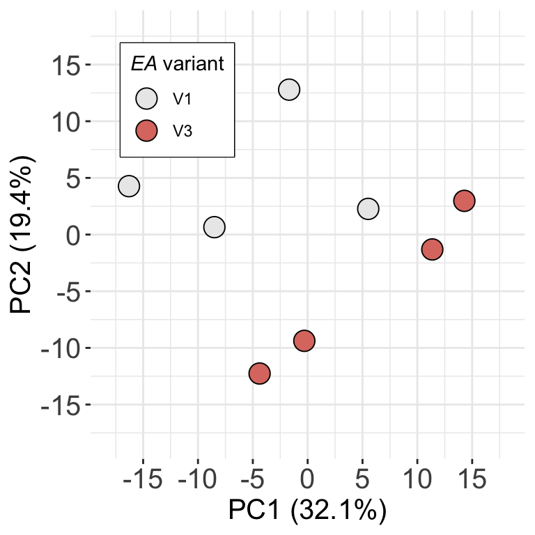
ggsave("../docs/FigS1D_PCA_plot.pdf", height =4, width = 4)PDF file: FigS1D_PCA_plot.pdf
Differential expression analysis
Differential expression using proDA
exprMat <- assay(fpeSub)
designMat <- model.matrix(~EA_variant, colData(fpeSub))
fit <- proDA(exprMat, design = designMat)
resTab <- test_diff(fit, contrast = "EA_variantV3") %>%
  arrange(pval) %>%
  mutate(symbol = rowData(fpeSub[name,])$name) %>%
  select(-name) %>%
  dplyr::rename(log2FC = diff) %>%
  select(symbol, pval, adj_pval, log2FC, t_statistic)
writexl::write_xlsx(resTab, "../docs/pTab_diffProt_V1V2.xlsx")
Result table: pTab_diffProt_V1V2.xlsx
Note that the list is not filtered. You can filter the list in
excel based on your cut-off
Volcano plot
plotTab <- resTab %>%
  mutate(ifSig = pval <= 0.05) %>%
  mutate(group = case_when(ifSig & log2FC >0 ~ "Higher in V3",
                           ifSig & log2FC <0 ~ "Higher in V1",
                           TRUE ~ "n.s."))

pVol <- ggplot(plotTab, aes(x= log2FC, y=-log10(pval))) +
  geom_point(aes(fill = group), shape =21, size=3) +
  geom_hline(yintercept = -log10(0.05), linetype = "dotted") +
  scale_fill_manual(values = c(`Higher in V1` = v1Color, `Higher in V3` = v3Color, n.s. = "grey30")) +
  scale_y_continuous(limits = c(0,4), breaks = seq(0,4), expand = c(0,0)) +
  xlim(-3,3) +
  ylab(bquote(-Log[10]*italic(P)*"-value"))+
  xlab(bquote(Log[2]*"LFQ intensity Fold Change"))+
  theme_classic() +
  theme(legend.position = "none",
        axis.text = element_text(size=16),
        axis.title = element_text(size=15))


gLegend <- ggplot(filter(plotTab, group != "n.s."),aes(x= log2FC, y=-log10(pval))) +
  geom_point(aes(fill = group), shape =21, size=4) +
  scale_fill_manual(values = c(`Higher in V1` = v1Color, `Higher in V3` = v3Color), name = NULL) +
  theme_classic() +
  theme(legend.position = "top",
        legend.background = element_rect(color = "black", linewidth = 0.3),
        legend.text = element_text(size=15))
pLegend <- cowplot::get_legend(gLegend)

pCom <- cowplot::plot_grid(pLegend, pVol, ncol=1, rel_heights = c(0.2,1))
pCom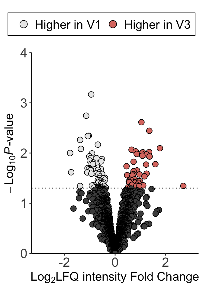
ggsave("../docs/Fig1E_volcano.pdf", height = 5, width = 3.5)PDF file: Fig1E_volcano.pdf
Enrichment analysis (pre-ranked GSEA)
#function for running gsea
# Run and plot enrichment barplot
runGSEA <- function(resTab, gmts, pCutSet = 0.1, geneFdr =FALSE, setFdr = TRUE,
                                 minSize = 15, maxSize = 400, nperm = 10000, collapsePathway = TRUE) {
  resInput <- resTab

  leadingEdgeTab <- tibble(Pathway=NULL, Gene = NULL, compare = NULL, setName = NULL)

  plotOut <- lapply(names(gmts), function(pathName) {
    print(paste0("Testing for: ", pathName))
    enList <- lapply(unique(resInput$compare), function(eachPair) {

      print(paste0("Condition: ", eachPair))

      inputTab <- filter(resInput, compare == eachPair, !symbol%in% c("",NA)) %>%
        arrange(pval) %>% distinct(symbol, .keep_all = TRUE) %>%
        select(symbol, t_statistic)
      geneList <- structure(inputTab$t_statistic, names = inputTab$symbol)
      setList <- fgsea::gmtPathways(gmts[[pathName]])

      fgRes <- fgsea::fgseaMultilevel(pathways = setList,
                              stats = geneList,
                              minSize=minSize, ## minimum gene set size
                              maxSize=maxSize) %>% arrange(pval)

      if (collapsePathway) {
          keepPath <- fgsea::collapsePathways(fgRes, setList, geneList)
          fgRes <- fgRes[fgRes$pathway %in% keepPath$mainPathways,]
      }

      #get number of leading edge gene
      fgRes$geneNum <- sapply(fgRes$leadingEdge, length)

      #get leading edge gene table
      eachLeadTab <- lapply(fgRes$pathway, function(eachPath) {
        tibble(Pathway = eachPath,
               Gene = fgRes[fgRes$pathway == eachPath,]$leadingEdge[[1]])
      }) %>% bind_rows() %>%
        mutate(compare = eachPair, setName = pathName)

      fgRes <- fgRes %>% select(pathway, pval, padj, NES, geneNum) %>% as_tibble()

      eachLeadTab <- filter(eachLeadTab, Pathway %in% fgRes$pathway)
      leadingEdgeTab <<- bind_rows(leadingEdgeTab, eachLeadTab)

      fgRes

    })

    names(enList) <- unique(resInput$compare)

    enList

  })

  names(plotOut) <- names(gmts)

  plotOut[["leadingEdgeGene"]] <- leadingEdgeTab

  return(plotOut)
}
Using Canonical pathway sets
resTab <- mutate(resTab, compare = "V3 versus V1")
gmts <- list(CanonicalPathway = "../data/gmts/m2.cp.v2022.1.Mm.symbols.gmt")
plotList <- runGSEA(resTab, gmts, pCutSet = 0.05, setFdr = FALSE)
[1] "Testing for: CanonicalPathway"
[1] "Condition: V3 versus V1"Table of enriched pathways (p-value < 0.05)
writexl::write_xlsx(plotList$CanonicalPathway$`V3 versus V1`, "../docs/GSEA_pathway_V1V3.xlsx")Plot
plotTab <- plotList$CanonicalPathway$`V3 versus V1` %>%
  arrange(NES) %>%
  mutate(pathway = str_remove_all(pathway, "WP|REACTOME|HALLMARK")) %>%
  mutate(pathway = str_replace_all(pathway, "_", " ")) %>%
  mutate(pathway = factor(pathway, levels = pathway))
ggplot(plotTab, aes(x=NES, y=pathway)) +
  geom_segment(aes(y=pathway, yend=pathway, x=0, xend=NES), color = "grey50")+
  geom_point(aes(color = padj, size = geneNum)) +
  scale_color_gradient(low = "navy", high = "red",
                       breaks = seq(0.05,0.2,0.05), limits=c(0.05, 0.22), name = "FDR") +
  scale_size_continuous(name = "SIZE") +
  ylab("") + xlab("Normalized enrichment score") +
  theme_bw() +
  theme(panel.border = element_blank(),
        axis.text.x = element_text(size=10))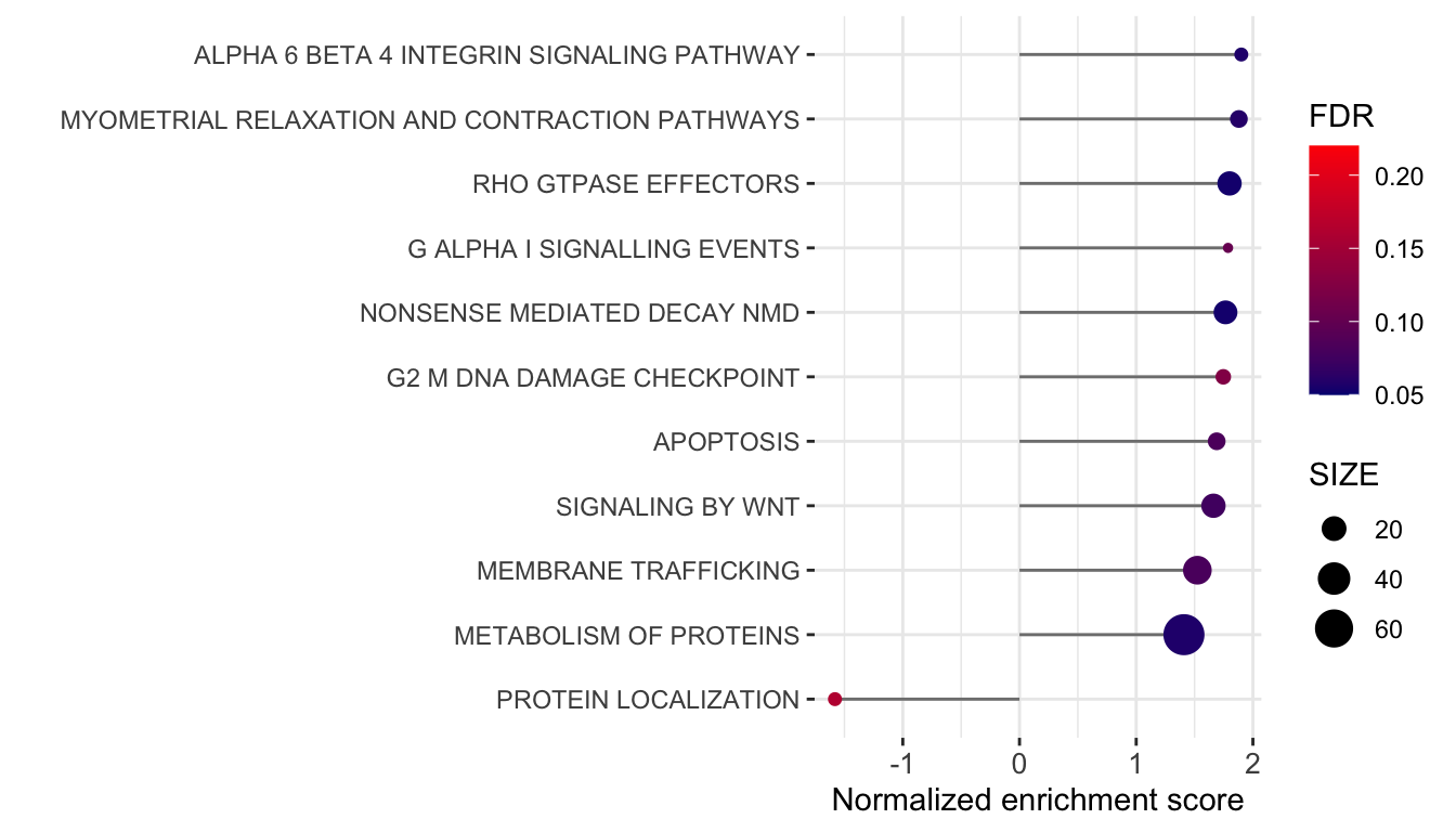
ggsave("../docs/Fig1G_GSEA.pdf", height = 4, width = 7)Positive enrichment score indicates upregulated in V3
PDF file: Fig1G_GSEA.pdf
Using Hallmark sets
resTab <- mutate(resTab, compare = "V3 versus V1")
gmts <- list(CanonicalPathway = "../data/gmts/mh.all.v2022.1.Mm.symbols.gmt")
plotList <- runGSEA(resTab, gmts, pCutSet = 0.05, setFdr = FALSE)
[1] "Testing for: CanonicalPathway"
[1] "Condition: V3 versus V1"Table of enriched pathways (p-value < 0.05)
writexl::write_xlsx(plotList$CanonicalPathway$`V3 versus V1`, "../docs/GSEA_Hallmark_V1V3.xlsx")Plot
plotTab <- plotList$CanonicalPathway$`V3 versus V1` %>%
  arrange(NES) %>%
  mutate(pathway = str_remove_all(pathway, "WP|REACTOME|HALLMARK")) %>%
  mutate(pathway = str_replace_all(pathway, "_", " ")) %>%
  mutate(pathway = factor(pathway, levels = pathway))
ggplot(plotTab, aes(x=NES, y=pathway)) +
  geom_segment(aes(y=pathway, yend=pathway, x=0, xend=NES), color = "grey50")+
  geom_point(aes(color = padj, size = geneNum)) +
  scale_color_gradient(low = "navy", high = "red",
                        name = "FDR") +
  scale_size_continuous(name = "SIZE") +
  ylab("") + xlab("Normalized enrichment score") +
  theme_bw() +
  theme(panel.border = element_blank(),
        axis.text.x = element_text(size=10))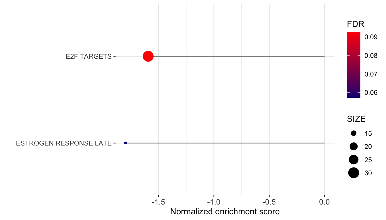
ggsave("../docs/Fig1G_GSEA_Hallmark.pdf", height = 4, width = 7)Positive enrichment score indicates upregulated in V3
PDF file: Fig1G_GSEA_Hallmark.pdf
For figure 5G: Brigatinib resistance cells versus sensitive cells (V3 only)
Preprocessing
Subsetting
fpeSub <- fpe[,fpe$treatment %in% c("dmso","brigatinib") & fpe$EA_variant == "V3"]
fpeSub$treatment <- factor(fpeSub$treatment, levels = c("dmso","brigatinib"))
fpeSub <- fpeSub[!rowData(fpeSub)$name %in% c(NA,""),]

keepVal <- rowSums(is.na(assay(fpeSub)))/ncol(fpeSub) <= 0.5
fpeSub <- fpeSub[keepVal,]

assay(fpeSub) <- log2(assay(fpeSub))
PCA plot (for a supplementary figure?)
#imputation for PCA
imp <- DEP::impute(fpeSub, "bpca")
assays(fpeSub)[["imputed"]] <- assay(imp)

exprMat <- assays(fpeSub)[["imputed"]]
smpAnno <- colData(fpeSub) %>% as_tibble()
pcRes <- prcomp(t(exprMat))
varExp <- pcRes$sdev^2/sum(pcRes$sdev^2)*100

pcTab <- pcRes$x[,1:2] %>%
    as_tibble(rownames = "sampleID") %>%
    left_join(smpAnno)

ggplot(pcTab, aes(x=PC1, y=PC2)) +
  geom_point(aes(fill = treatment), shape = 21, size=5) +
  scale_fill_manual(values = c(dmso = v1Color, brigatinib= v3Color), name = "treatment")+
  scale_x_continuous(limits = c(-20,20), breaks = seq(-20,20,5)) +
  scale_y_continuous(limits = c(-20,20), breaks = seq(-20,20,5)) +
  xlab(sprintf("PC1 (%1.1f%%)",varExp[1])) +
  ylab(sprintf("PC2 (%1.1f%%)",varExp[2])) +
  theme_bw() +
  theme(panel.border = element_blank(),
        legend.position = c(0.8,0.85),
        legend.box.background  = element_rect(),
        axis.title = element_text(size=15),
        axis.text = element_text(size=15))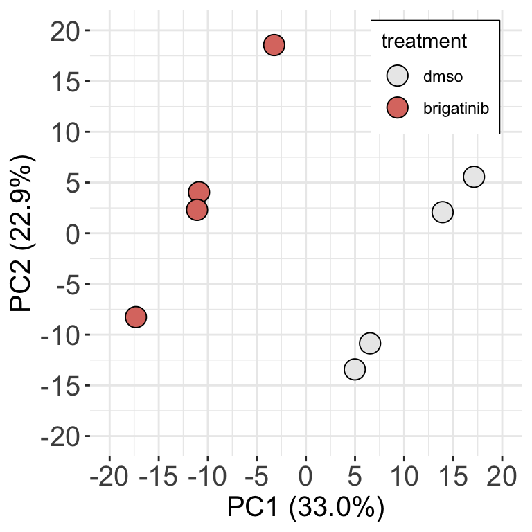
ggsave("../docs/briga_DMSO_PCA_plot.pdf", height =4, width = 4)PDF file: briga_DMSO_PCA_plot.pdf
Differential expression test (briga versus dmso in V3)
exprMat <- assay(fpeSub)
designMat <- model.matrix(~treatment, colData(fpeSub))
fit <- proDA(exprMat, design = designMat)
resTab <- test_diff(fit, contrast = "treatmentbrigatinib") %>%
  arrange(pval) %>%
  mutate(symbol = rowData(fpeSub[name,])$name) %>%
  select(-name) %>%
  dplyr::rename(log2FC = diff) %>%
  select(symbol, pval, adj_pval, log2FC, t_statistic)
writexl::write_xlsx(resTab, "../docs/pTab_diffProt_briga_dmso.xlsx")
Result table: pTab_diffProt_briga_dmso.xlsx
Note that the list is not filtered. You can filter the list in
excel based on your cut-off
Positive logFC means proteins are up-regulated in brigatinib
treatment cells
Enrichment analysis (pre-ranked GSEA)
Using Canonical pathways
resTab <- mutate(resTab, compare = "brigatinib versus dmso")
gmts <- list(CanonicalPathway = "../data/gmts/m2.cp.v2022.1.Mm.symbols.gmt")
plotList <- runGSEA(resTab, gmts, pCutSet = 0.05, setFdr = FALSE)
[1] "Testing for: CanonicalPathway"
[1] "Condition: brigatinib versus dmso"Table of enriched pathways (p-value < 0.05)
writexl::write_xlsx(plotList$CanonicalPathway$`brigatinib versus dmso`, "../docs/GSEA_pathway_brigaResistant.xlsx")Plot
plotTab <- plotList$CanonicalPathway$`brigatinib versus dmso` %>%
  arrange(NES) %>%
  mutate(pathway = str_remove_all(pathway, "WP|REACTOME")) %>%
  mutate(pathway = str_replace_all(pathway, "_", " ")) %>%
  mutate(pathway = factor(pathway, levels = pathway))
ggplot(plotTab, aes(x=NES, y=pathway)) +
  geom_segment(aes(y=pathway, yend=pathway, x=0, xend=NES), color = "grey50")+
  geom_point(aes(color = padj, size = geneNum)) +
  scale_color_gradient(low = "navy", high = "red",
                       breaks = seq(0.00,0.2,0.05), limits=c(0.00, 0.22), name = "FDR") +
  scale_size_continuous(name = "SIZE") +
  ylab("") + xlab("Normalized enrichment score") +
  theme_bw() +
  theme(panel.border = element_blank(),
        axis.text.x = element_text(size=10))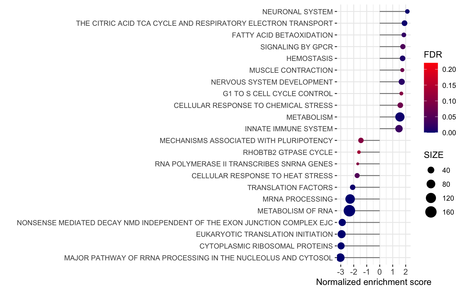
ggsave("../docs/BrigaResistant_GSEA.pdf", height = 5, width = 8)Positive enrichment score indicates upregulated in brigatinib resistant
PDF file: BrigaResistant_GSEA.pdf
Using Hallmark
resTab <- mutate(resTab, compare = "brigatinib versus dmso")
gmts <- list(CanonicalPathway = "../data/gmts/mh.all.v2022.1.Mm.symbols.gmt")
plotList <- runGSEA(resTab, gmts, pCutSet = 0.05, setFdr = FALSE)
[1] "Testing for: CanonicalPathway"
[1] "Condition: brigatinib versus dmso"Table of enriched pathways (p-value < 0.05)
writexl::write_xlsx(plotList$CanonicalPathway$`brigatinib versus dmso`, "../docs/GSEA_Hallmark_brigaResistant.xlsx")Plot
plotTab <- plotList$CanonicalPathway$`brigatinib versus dmso` %>%
  arrange(NES) %>%
  mutate(pathway = str_remove_all(pathway, "WP|REACTOME|HALLMARK")) %>%
  mutate(pathway = str_replace_all(pathway, "_", " ")) %>%
  mutate(pathway = factor(pathway, levels = pathway))
ggplot(plotTab, aes(x=NES, y=pathway)) +
  geom_segment(aes(y=pathway, yend=pathway, x=0, xend=NES), color = "grey50")+
  geom_point(aes(color = padj, size = geneNum)) +
  scale_color_gradient(low = "navy", high = "red",
                      name = "FDR") +
  scale_size_continuous(name = "SIZE") +
  ylab("") + xlab("Normalized enrichment score") +
  theme_bw() +
  theme(panel.border = element_blank(),
        axis.text.x = element_text(size=10))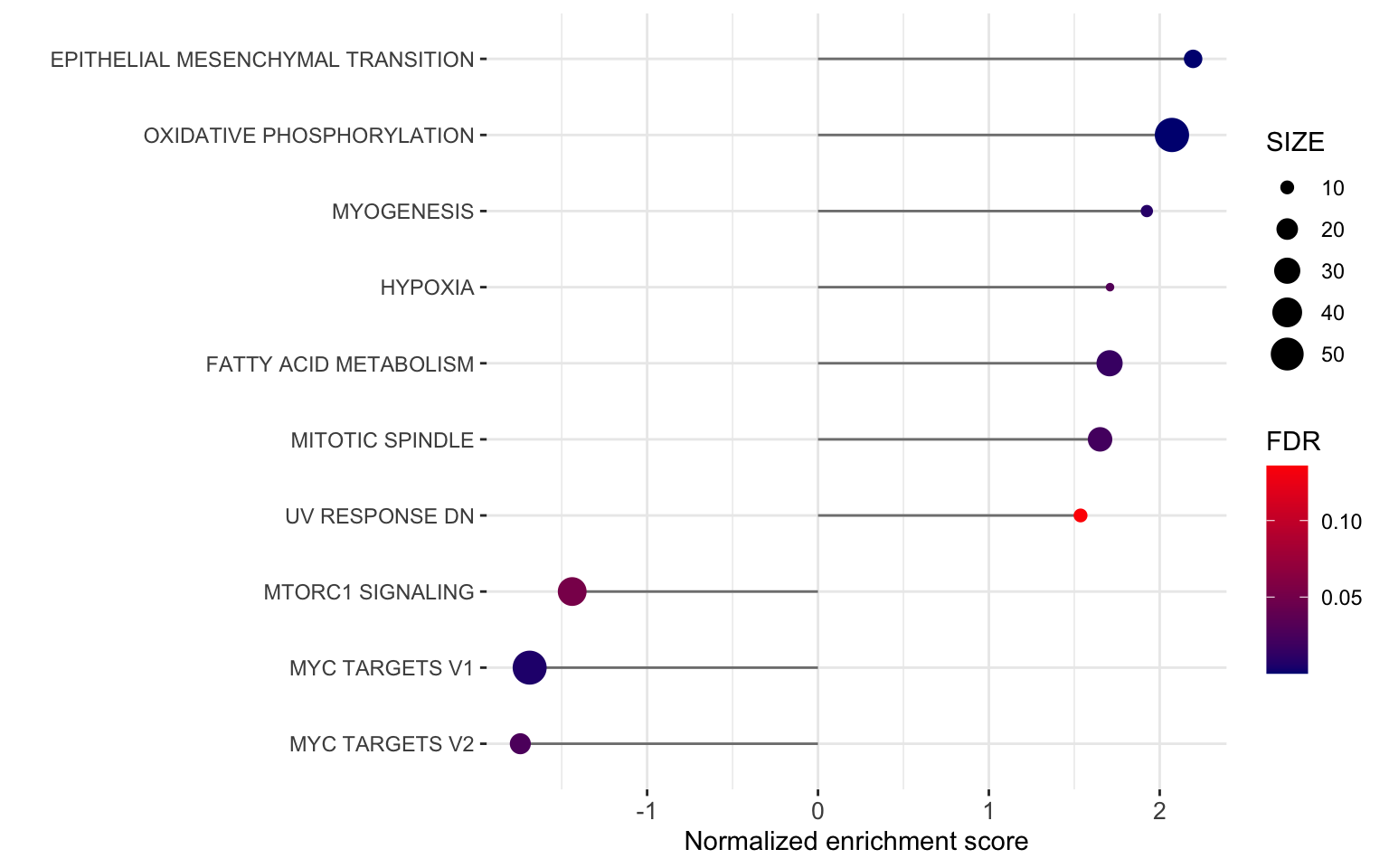
ggsave("../docs/BrigaResistant_GSEA_Hallmark.pdf", height = 5, width = 8)PDF file: BrigaResistant_GSEA_Hallmark.pdf
List of proteins up-regulated in brigatinib resistant cell lines and down-regulated in combo compared to brigatinib
Define a list of up-regulated proteins in resistant cell lines (using p-value < 0.05, log2FC > 0)
resTab.up <- resTab %>% filter(pval < 0.05, log2FC > 0) %>%
  arrange(pval) %>% distinct(symbol, .keep_all = TRUE) %>%
  dplyr::rename(`pval (briga resistace)` = pval, `log2FC (briga resistance)`= log2FC) %>%
  select(-adj_pval, -t_statistic)
DE list of combo versus brigatinib at 16 hours
load("../output/allResList_RUN5_timeBased.RData")
deTab.comboDown <- allResList$diffProt$time_16 %>% filter(compare == "combo_brigatinib") %>%
  filter(pval < 0.05, diff <0) %>%
  arrange(pval) %>% distinct(symbol, .keep_all = TRUE) %>%
  dplyr::rename(`pval (combo vs briga)` = pval, `log2FC (combo vs briga)`= diff) %>%
  select(-adj_pval, -t_statistic, -name, -compare)
Table of common proteins
overlap <- intersect(resTab.up$symbol, deTab.comboDown$symbol)

comTab <- left_join(filter(resTab.up,symbol %in% overlap),
                    filter(deTab.comboDown, symbol %in% overlap), by = "symbol")

writexl::write_xlsx(comTab, "../docs/overlap_protein_list_briga_combo.xlsx")
overlap_protein_list_briga_combo.xlsx
sessionInfo()R version 4.2.0 (2022-04-22)
Platform: x86_64-apple-darwin17.0 (64-bit)
Running under: macOS Big Sur/Monterey 10.16
Matrix products: default
BLAS: /Library/Frameworks/R.framework/Versions/4.2/Resources/lib/libRblas.0.dylib
LAPACK: /Library/Frameworks/R.framework/Versions/4.2/Resources/lib/libRlapack.dylib
locale:
[1] en_US.UTF-8/en_US.UTF-8/en_US.UTF-8/C/en_US.UTF-8/en_US.UTF-8
attached base packages:
[1] stats4 stats graphics grDevices utils datasets methods
[8] base
other attached packages:
[1] forcats_0.5.1 stringr_1.4.1
[3] dplyr_1.0.9 purrr_0.3.4
[5] readr_2.1.2 tidyr_1.2.0
[7] tibble_3.1.8 ggplot2_3.4.1
[9] tidyverse_1.3.2 proDA_1.10.0
[11] MultiAssayExperiment_1.22.0 SummarizedExperiment_1.26.1
[13] Biobase_2.56.0 GenomicRanges_1.48.0
[15] GenomeInfoDb_1.32.2 IRanges_2.30.0
[17] S4Vectors_0.34.0 BiocGenerics_0.42.0
[19] MatrixGenerics_1.8.1 matrixStats_0.62.0
[21] DEP_1.18.0
loaded via a namespace (and not attached):
[1] readxl_1.4.0 backports_1.4.1 circlize_0.4.15
[4] fastmatch_1.1-3 workflowr_1.7.0 systemfonts_1.0.4
[7] plyr_1.8.7 gmm_1.6-6 shinydashboard_0.7.2
[10] BiocParallel_1.30.3 digest_0.6.30 foreach_1.5.2
[13] htmltools_0.5.4 fansi_1.0.3 magrittr_2.0.3
[16] googlesheets4_1.0.0 cluster_2.1.3 doParallel_1.0.17
[19] tzdb_0.3.0 limma_3.52.2 ComplexHeatmap_2.12.0
[22] modelr_0.1.8 imputeLCMD_2.1 sandwich_3.0-2
[25] colorspace_2.0-3 rvest_1.0.2 textshaping_0.3.6
[28] haven_2.5.0 xfun_0.31 crayon_1.5.2
[31] RCurl_1.98-1.7 jsonlite_1.8.3 impute_1.70.0
[34] zoo_1.8-10 iterators_1.0.14 glue_1.6.2
[37] gtable_0.3.0 gargle_1.2.0 zlibbioc_1.42.0
[40] XVector_0.36.0 GetoptLong_1.0.5 DelayedArray_0.22.0
[43] shape_1.4.6 scales_1.2.0 vsn_3.64.0
[46] mvtnorm_1.1-3 DBI_1.1.3 Rcpp_1.0.9
[49] mzR_2.30.0 xtable_1.8-4 clue_0.3-61
[52] preprocessCore_1.58.0 MsCoreUtils_1.8.0 DT_0.23
[55] htmlwidgets_1.5.4 httr_1.4.3 fgsea_1.22.0
[58] RColorBrewer_1.1-3 ellipsis_0.3.2 farver_2.1.1
[61] pkgconfig_2.0.3 XML_3.99-0.10 sass_0.4.2
[64] dbplyr_2.2.1 utf8_1.2.2 labeling_0.4.2
[67] tidyselect_1.1.2 rlang_1.0.6 later_1.3.0
[70] munsell_0.5.0 cellranger_1.1.0 tools_4.2.0
[73] cachem_1.0.6 cli_3.4.1 generics_0.1.3
[76] broom_1.0.0 evaluate_0.15 fastmap_1.1.0
[79] ragg_1.2.2 mzID_1.34.0 yaml_2.3.5
[82] knitr_1.39 fs_1.5.2 ncdf4_1.19
[85] mime_0.12 xml2_1.3.3 compiler_4.2.0
[88] rstudioapi_0.13 png_0.1-7 affyio_1.66.0
[91] reprex_2.0.1 bslib_0.4.1 stringi_1.7.8
[94] highr_0.9 MSnbase_2.22.0 lattice_0.20-45
[97] ProtGenerics_1.28.0 Matrix_1.5-4 tmvtnorm_1.5
[100] vctrs_0.5.2 pillar_1.8.0 norm_1.0-10.0
[103] lifecycle_1.0.3 BiocManager_1.30.18 jquerylib_0.1.4
[106] MALDIquant_1.21 GlobalOptions_0.1.2 data.table_1.14.8
[109] cowplot_1.1.1 bitops_1.0-7 httpuv_1.6.6
[112] extraDistr_1.9.1 R6_2.5.1 pcaMethods_1.88.0
[115] affy_1.74.0 promises_1.2.0.1 gridExtra_2.3
[118] writexl_1.4.0 codetools_0.2-18 MASS_7.3-58
[121] assertthat_0.2.1 rprojroot_2.0.3 rjson_0.2.21
[124] withr_2.5.0 GenomeInfoDbData_1.2.8 parallel_4.2.0
[127] hms_1.1.1 grid_4.2.0 rmarkdown_2.14
[130] googledrive_2.0.0 git2r_0.30.1 shiny_1.7.4
[133] lubridate_1.8.0