Read and process data
Last updated: 2022-11-17
Checks: 4 2
Knit directory:
LungCancer_SotilloLab/analysis/
This reproducible R Markdown analysis was created with workflowr (version 1.7.0). The Checks tab describes the reproducibility checks that were applied when the results were created. The Past versions tab lists the development history.
Great job! The global environment was empty. Objects defined in the global environment can affect the analysis in your R Markdown file in unknown ways. For reproduciblity it’s best to always run the code in an empty environment.
The command set.seed(20221103) was run prior to running
the code in the R Markdown file. Setting a seed ensures that any results
that rely on randomness, e.g. subsampling or permutations, are
reproducible.
Great job! Recording the operating system, R version, and package versions is critical for reproducibility.
- unnamed-chunk-50
- unnamed-chunk-68
- unnamed-chunk-73
To ensure reproducibility of the results, delete the cache directory
process_cache and re-run the analysis. To have workflowr
automatically delete the cache directory prior to building the file, set
delete_cache = TRUE when running wflow_build()
or wflow_publish().
Great job! Using relative paths to the files within your workflowr project makes it easier to run your code on other machines.
Tracking code development and connecting the code version to the
results is critical for reproducibility. To start using Git, open the
Terminal and type git init in your project directory.
This project is not being versioned with Git. To obtain the full
reproducibility benefits of using workflowr, please see
?wflow_start.
Load packages and dataset
#package
library(SmartPhos)
library(PhosR)
Registered S3 method overwritten by 'GGally':
method from
+.gg ggplot2library(DEP)Warning in fun(libname, pkgname): mzR has been built against a different Rcpp version (1.0.8.3)
than is installed on your system (1.0.9). This might lead to errors
when loading mzR. If you encounter such issues, please send a report,
including the output of sessionInfo() to the Bioc support forum at
https://support.bioconductor.org/. For details see also
https://github.com/sneumann/mzR/wiki/mzR-Rcpp-compiler-linker-issue.library(SummarizedExperiment)Loading required package: MatrixGenericsLoading required package: matrixStats
Attaching package: 'MatrixGenerics'The following objects are masked from 'package:matrixStats':
colAlls, colAnyNAs, colAnys, colAvgsPerRowSet, colCollapse,
colCounts, colCummaxs, colCummins, colCumprods, colCumsums,
colDiffs, colIQRDiffs, colIQRs, colLogSumExps, colMadDiffs,
colMads, colMaxs, colMeans2, colMedians, colMins, colOrderStats,
colProds, colQuantiles, colRanges, colRanks, colSdDiffs, colSds,
colSums2, colTabulates, colVarDiffs, colVars, colWeightedMads,
colWeightedMeans, colWeightedMedians, colWeightedSds,
colWeightedVars, rowAlls, rowAnyNAs, rowAnys, rowAvgsPerColSet,
rowCollapse, rowCounts, rowCummaxs, rowCummins, rowCumprods,
rowCumsums, rowDiffs, rowIQRDiffs, rowIQRs, rowLogSumExps,
rowMadDiffs, rowMads, rowMaxs, rowMeans2, rowMedians, rowMins,
rowOrderStats, rowProds, rowQuantiles, rowRanges, rowRanks,
rowSdDiffs, rowSds, rowSums2, rowTabulates, rowVarDiffs, rowVars,
rowWeightedMads, rowWeightedMeans, rowWeightedMedians,
rowWeightedSds, rowWeightedVarsLoading required package: GenomicRangesLoading required package: stats4Loading required package: BiocGenerics
Attaching package: 'BiocGenerics'The following objects are masked from 'package:stats':
IQR, mad, sd, var, xtabsThe following objects are masked from 'package:base':
anyDuplicated, append, as.data.frame, basename, cbind, colnames,
dirname, do.call, duplicated, eval, evalq, Filter, Find, get, grep,
grepl, intersect, is.unsorted, lapply, Map, mapply, match, mget,
order, paste, pmax, pmax.int, pmin, pmin.int, Position, rank,
rbind, Reduce, rownames, sapply, setdiff, sort, table, tapply,
union, unique, unsplit, which.max, which.minLoading required package: S4Vectors
Attaching package: 'S4Vectors'The following objects are masked from 'package:base':
expand.grid, I, unnameLoading required package: IRangesLoading required package: GenomeInfoDbLoading required package: BiobaseWelcome to Bioconductor
Vignettes contain introductory material; view with
'browseVignettes()'. To cite Bioconductor, see
'citation("Biobase")', and for packages 'citation("pkgname")'.
Attaching package: 'Biobase'The following object is masked from 'package:MatrixGenerics':
rowMediansThe following objects are masked from 'package:matrixStats':
anyMissing, rowMedianslibrary(tidyverse)── Attaching packages
───────────────────────────────────────
tidyverse 1.3.2 ──✔ ggplot2 3.3.6 ✔ purrr 0.3.4
✔ tibble 3.1.8 ✔ dplyr 1.0.9
✔ tidyr 1.2.0 ✔ stringr 1.4.1
✔ readr 2.1.2 ✔ forcats 0.5.1
── Conflicts ────────────────────────────────────────── tidyverse_conflicts() ──
✖ dplyr::collapse() masks IRanges::collapse()
✖ dplyr::combine() masks Biobase::combine(), BiocGenerics::combine()
✖ dplyr::count() masks matrixStats::count()
✖ dplyr::desc() masks IRanges::desc()
✖ tidyr::expand() masks S4Vectors::expand()
✖ dplyr::filter() masks stats::filter()
✖ dplyr::first() masks S4Vectors::first()
✖ dplyr::lag() masks stats::lag()
✖ ggplot2::Position() masks BiocGenerics::Position(), base::Position()
✖ purrr::reduce() masks GenomicRanges::reduce(), IRanges::reduce()
✖ dplyr::rename() masks S4Vectors::rename()
✖ dplyr::slice() masks IRanges::slice()Create input file table manually
Proteomics
protInfo <- tibble(cols= colnames(data.table::fread("../data/20221021_Lung_Mouse_CellLines_Phospho_TimeCourse_SUP_OTEC_SotilloCollab_SN16.2/20221021_072758_20221019_EA_LungTumor_CellLines_Mouse_Phospho_SotilloCollab_SN16.2_Protein_Report.xls", check.names = TRUE))) %>%
    filter(str_detect(cols, "PG.Quantity")) %>%
    mutate(id = str_remove(cols, ".raw.PG.Quantity")) %>%
    separate(id, into = LETTERS[1:10], sep = "_", remove = FALSE) %>%
    dplyr::rename(sampleType = A, cellLine = E, drug = B, time = C, replicate = F) %>%
    select(id, sampleType, cellLine, drug, time, replicate ) %>%
    mutate(sampleType = ifelse(str_detect(sampleType, "FP"), "FP", "PP"),
           sampleCondi = paste0(cellLine,"_", drug,"_", time),
           fileName = file.path("../data/20221021_Lung_Mouse_CellLines_Phospho_TimeCourse_SUP_OTEC_SotilloCollab_SN16.2/20221021_072758_20221019_EA_LungTumor_CellLines_Mouse_Phospho_SotilloCollab_SN16.2_Protein_Report.xls"),
           type = "proteome")
Warning: Expected 10 pieces. Missing pieces filled with `NA` in 192 rows [1, 2,
3, 4, 5, 6, 7, 8, 9, 10, 11, 12, 13, 14, 15, 16, 17, 18, 19, 20, ...].Phospho-proteomics
phosInfo <- tibble(cols= colnames(data.table::fread("../data/20221021_Lung_Mouse_CellLines_Phospho_TimeCourse_SUP_OTEC_SotilloCollab_SN16.2/20221021_085606_20221019_EA_LungTumor_CellLines_Mouse_Phospho_SotilloCollab_SN16.2_Phospho_Report.xls",check.names = TRUE))) %>%
    filter(str_detect(cols, "PTM.Quantity")) %>%
    mutate(id = str_remove(cols, ".raw.PTM.Quantity")) %>%
    mutate(id = str_replace_all(id, "[+]",".")) %>%
    separate(id, into = LETTERS[1:10], sep = "_", remove = FALSE) %>%
    dplyr::rename(sampleType = A, cellLine = E, drug = B, time = C, replicate = F) %>%
    select(id, sampleType, cellLine, drug, time, replicate ) %>%
    mutate(sampleType = ifelse(str_detect(sampleType, "FP"), "FP", "PP"),
           sampleCondi = paste0(cellLine,"_", drug,"_", time),
           fileName = file.path("../data/20221021_Lung_Mouse_CellLines_Phospho_TimeCourse_SUP_OTEC_SotilloCollab_SN16.2/20221021_085606_20221019_EA_LungTumor_CellLines_Mouse_Phospho_SotilloCollab_SN16.2_Phospho_Report.xls"),
           type = "phosphoproteome")
Warning: Expected 10 pieces. Missing pieces filled with `NA` in 192 rows [1, 2,
3, 4, 5, 6, 7, 8, 9, 10, 11, 12, 13, 14, 15, 16, 17, 18, 19, 20, ...].Combine
fileTable <- bind_rows(protInfo, phosInfo) %>%
    mutate(time = as.numeric(str_remove(time,"h"))) %>%
    data.frame()
Parse the whole experiment using the readExperiment function from SmartPhos
testData <- readExperimentDIA(fileTable, annotation_col = c("cellLine","sampleType","drug","time", "replicate","sampleCondi"))[1] "Processing phosphoproteomic data"
|
| | 0%
|
| | 1%
|
|= | 1%
|
|= | 2%
|
|== | 3%
|
|=== | 4%
|
|=== | 5%
|
|==== | 5%
|
|==== | 6%
|
|===== | 7%
|
|===== | 8%
|
|====== | 8%
|
|====== | 9%
|
|======= | 9%
|
|======= | 10%
|
|======== | 11%
|
|======== | 12%
|
|========= | 12%
|
|========= | 13%
|
|========= | 14%
|
|========== | 14%
|
|========== | 15%
|
|=========== | 15%
|
|=========== | 16%
|
|============ | 17%
|
|============ | 18%
|
|============= | 18%
|
|============= | 19%
|
|============== | 20%
|
|=============== | 21%
|
|=============== | 22%
|
|================ | 22%
|
|================ | 23%
|
|================= | 24%
|
|================== | 25%
|
|================== | 26%
|
|=================== | 27%
|
|=================== | 28%
|
|==================== | 28%
|
|==================== | 29%
|
|===================== | 30%
|
|====================== | 31%
|
|====================== | 32%
|
|======================= | 32%
|
|======================= | 33%
|
|======================== | 34%
|
|======================== | 35%
|
|========================= | 35%
|
|========================= | 36%
|
|========================== | 36%
|
|========================== | 37%
|
|========================== | 38%
|
|=========================== | 38%
|
|=========================== | 39%
|
|============================ | 40%
|
|============================ | 41%
|
|============================= | 41%
|
|============================= | 42%
|
|============================== | 42%
|
|============================== | 43%
|
|=============================== | 44%
|
|=============================== | 45%
|
|================================ | 45%
|
|================================ | 46%
|
|================================= | 47%
|
|================================== | 48%
|
|================================== | 49%
|
|=================================== | 49%
|
|=================================== | 50%
|
|=================================== | 51%
|
|==================================== | 51%
|
|==================================== | 52%
|
|===================================== | 53%
|
|====================================== | 54%
|
|====================================== | 55%
|
|======================================= | 55%
|
|======================================= | 56%
|
|======================================== | 57%
|
|======================================== | 58%
|
|========================================= | 58%
|
|========================================= | 59%
|
|========================================== | 59%
|
|========================================== | 60%
|
|=========================================== | 61%
|
|=========================================== | 62%
|
|============================================ | 62%
|
|============================================ | 63%
|
|============================================ | 64%
|
|============================================= | 64%
|
|============================================= | 65%
|
|============================================== | 65%
|
|============================================== | 66%
|
|=============================================== | 67%
|
|=============================================== | 68%
|
|================================================ | 68%
|
|================================================ | 69%
|
|================================================= | 70%
|
|================================================== | 71%
|
|================================================== | 72%
|
|=================================================== | 72%
|
|=================================================== | 73%
|
|==================================================== | 74%
|
|==================================================== | 75%
|
|===================================================== | 76%
|
|====================================================== | 77%
|
|====================================================== | 78%
|
|======================================================= | 78%
|
|======================================================= | 79%
|
|======================================================== | 80%
|
|========================================================= | 81%
|
|========================================================= | 82%
|
|========================================================== | 82%
|
|========================================================== | 83%
|
|=========================================================== | 84%
|
|=========================================================== | 85%
|
|============================================================ | 85%
|
|============================================================ | 86%
|
|============================================================= | 86%
|
|============================================================= | 87%
|
|============================================================= | 88%
|
|============================================================== | 88%
|
|============================================================== | 89%
|
|=============================================================== | 90%
|
|=============================================================== | 91%
|
|================================================================ | 91%
|
|================================================================ | 92%
|
|================================================================= | 92%
|
|================================================================= | 93%
|
|================================================================== | 94%
|
|================================================================== | 95%
|
|=================================================================== | 95%
|
|=================================================================== | 96%
|
|==================================================================== | 97%
|
|===================================================================== | 98%
|
|===================================================================== | 99%
|
|======================================================================| 99%
|
|======================================================================| 100%
[1] "Processing proteomic data"
|
| | 0%
|
| | 1%
|
|= | 1%
|
|= | 2%
|
|== | 3%
|
|=== | 4%
|
|=== | 5%
|
|==== | 5%
|
|==== | 6%
|
|===== | 7%
|
|===== | 8%
|
|====== | 8%
|
|====== | 9%
|
|======= | 9%
|
|======= | 10%
|
|======== | 11%
|
|======== | 12%
|
|========= | 12%
|
|========= | 13%
|
|========= | 14%
|
|========== | 14%
|
|========== | 15%
|
|=========== | 15%
|
|=========== | 16%
|
|============ | 17%
|
|============ | 18%
|
|============= | 18%
|
|============= | 19%
|
|============== | 20%
|
|=============== | 21%
|
|=============== | 22%
|
|================ | 22%
|
|================ | 23%
|
|================= | 24%
|
|================== | 25%
|
|================== | 26%
|
|=================== | 27%
|
|=================== | 28%
|
|==================== | 28%
|
|==================== | 29%
|
|===================== | 30%
|
|====================== | 31%
|
|====================== | 32%
|
|======================= | 32%
|
|======================= | 33%
|
|======================== | 34%
|
|======================== | 35%
|
|========================= | 35%
|
|========================= | 36%
|
|========================== | 36%
|
|========================== | 37%
|
|========================== | 38%
|
|=========================== | 38%
|
|=========================== | 39%
|
|============================ | 40%
|
|============================ | 41%
|
|============================= | 41%
|
|============================= | 42%
|
|============================== | 42%
|
|============================== | 43%
|
|=============================== | 44%
|
|=============================== | 45%
|
|================================ | 45%
|
|================================ | 46%
|
|================================= | 47%
|
|================================== | 48%
|
|================================== | 49%
|
|=================================== | 49%
|
|=================================== | 50%
|
|=================================== | 51%
|
|==================================== | 51%
|
|==================================== | 52%
|
|===================================== | 53%
|
|====================================== | 54%
|
|====================================== | 55%
|
|======================================= | 55%
|
|======================================= | 56%
|
|======================================== | 57%
|
|======================================== | 58%
|
|========================================= | 58%
|
|========================================= | 59%
|
|========================================== | 59%
|
|========================================== | 60%
|
|=========================================== | 61%
|
|=========================================== | 62%
|
|============================================ | 62%
|
|============================================ | 63%
|
|============================================ | 64%
|
|============================================= | 64%
|
|============================================= | 65%
|
|============================================== | 65%
|
|============================================== | 66%
|
|=============================================== | 67%
|
|=============================================== | 68%
|
|================================================ | 68%
|
|================================================ | 69%
|
|================================================= | 70%
|
|================================================== | 71%
|
|================================================== | 72%
|
|=================================================== | 72%
|
|=================================================== | 73%
|
|==================================================== | 74%
|
|==================================================== | 75%
|
|===================================================== | 76%
|
|====================================================== | 77%
|
|====================================================== | 78%
|
|======================================================= | 78%
|
|======================================================= | 79%
|
|======================================================== | 80%
|
|========================================================= | 81%
|
|========================================================= | 82%
|
|========================================================== | 82%
|
|========================================================== | 83%
|
|=========================================================== | 84%
|
|=========================================================== | 85%
|
|============================================================ | 85%
|
|============================================================ | 86%
|
|============================================================= | 86%
|
|============================================================= | 87%
|
|============================================================= | 88%
|
|============================================================== | 88%
|
|============================================================== | 89%
|
|=============================================================== | 90%
|
|=============================================================== | 91%
|
|================================================================ | 91%
|
|================================================================ | 92%
|
|================================================================= | 92%
|
|================================================================= | 93%
|
|================================================================== | 94%
|
|================================================================== | 95%
|
|=================================================================== | 95%
|
|=================================================================== | 96%
|
|==================================================================== | 97%
|
|===================================================================== | 98%
|
|===================================================================== | 99%
|
|======================================================================| 99%
|
|======================================================================| 100%Check the data
testDataA MultiAssayExperiment object of 2 listed
experiments with user-defined names and respective classes.
Containing an ExperimentList class object of length 2:
[1] Phosphoproteome: SummarizedExperiment with 20702 rows and 192 columns
[2] Proteome: SummarizedExperiment with 8699 rows and 192 columns
Functionality:
experiments() - obtain the ExperimentList instance
colData() - the primary/phenotype DataFrame
sampleMap() - the sample coordination DataFrame
`$`, `[`, `[[` - extract colData columns, subset, or experiment
*Format() - convert into a long or wide DataFrame
assays() - convert ExperimentList to a SimpleList of matrices
exportClass() - save data to flat filesmaeData <- testData
maeData$sample <- paste0(maeData$sampleCondi, "_", maeData$replicate)Check phosphoproteome data distribution
Subset for phosphoproteomic data
ppe <- maeData[["Phosphoproteome"]]
colData(ppe) <- colData(maeData)
Examin the data distrubution
countMat <- assay(ppe)Missing value per sample
plotTab <- tibble(sample = ppe$sample,
                  perNA = colSums(is.na(countMat))/nrow(countMat),
                  total = colSums(countMat, na.rm=TRUE),
                  medVal = colMedians(countMat, na.rm=TRUE),
                  type = ppe$sampleType,
                  time = ppe$time,
                  drug = ppe$drug)
ggplot(plotTab, aes(x=sample, y=1-perNA, fill = time)) +
    geom_bar(stat = "identity") +
    ylab("completeness") +
    theme(axis.text.x = element_text(angle = 90, hjust = 1, vjust=0)) +
    facet_wrap(~type+drug, scale = "free_x", ncol=4)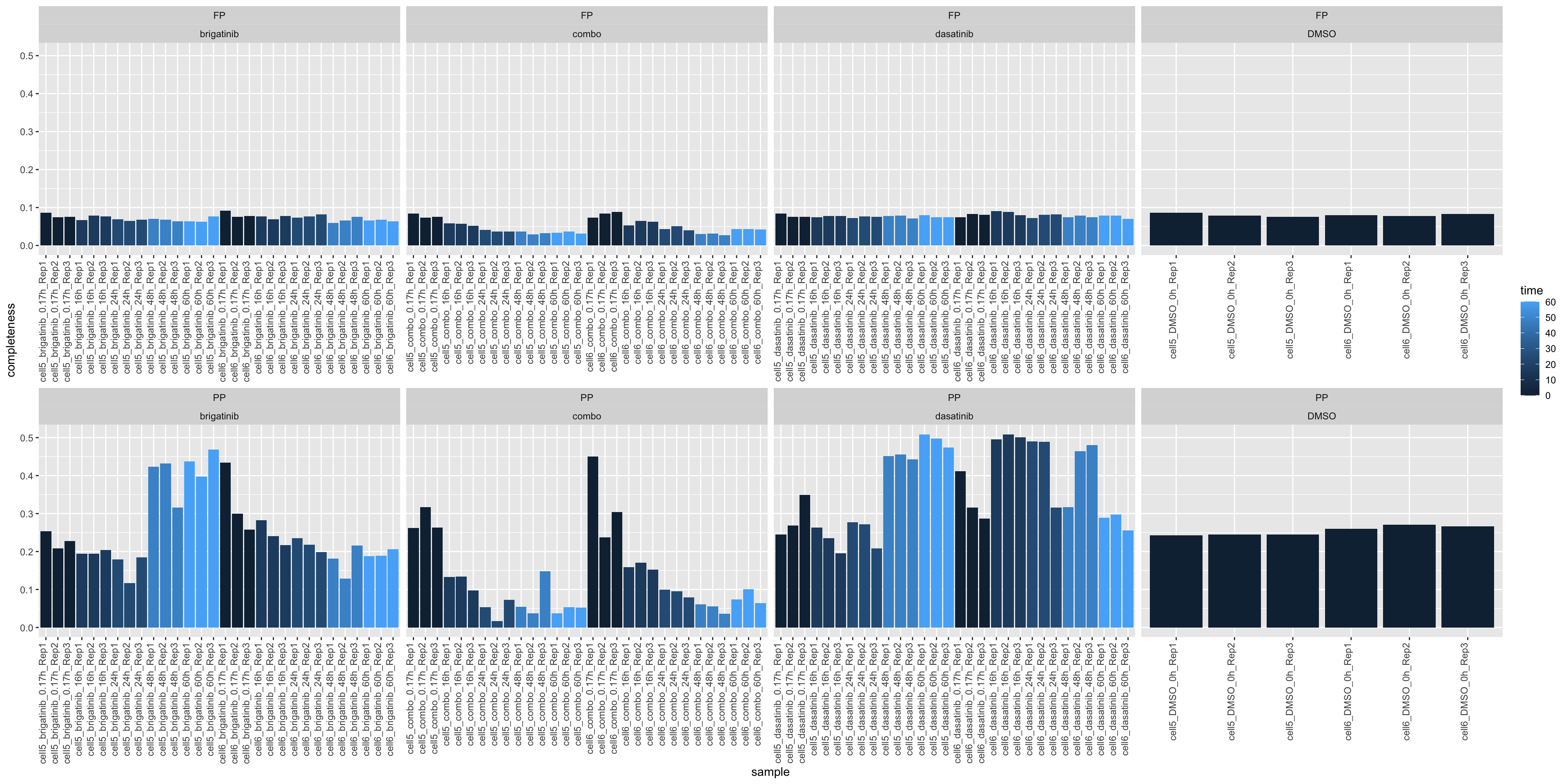
Total intensity
ggplot(plotTab, aes(x=sample, y=total, fill = time)) +
    geom_bar(stat = "identity") +
    ylab("completeness") +
    theme(axis.text.x = element_text(angle = 90, hjust = 1, vjust=0)) +
    facet_wrap(~type+drug, scale = "free_x", ncol=4) +
    scale_y_log10()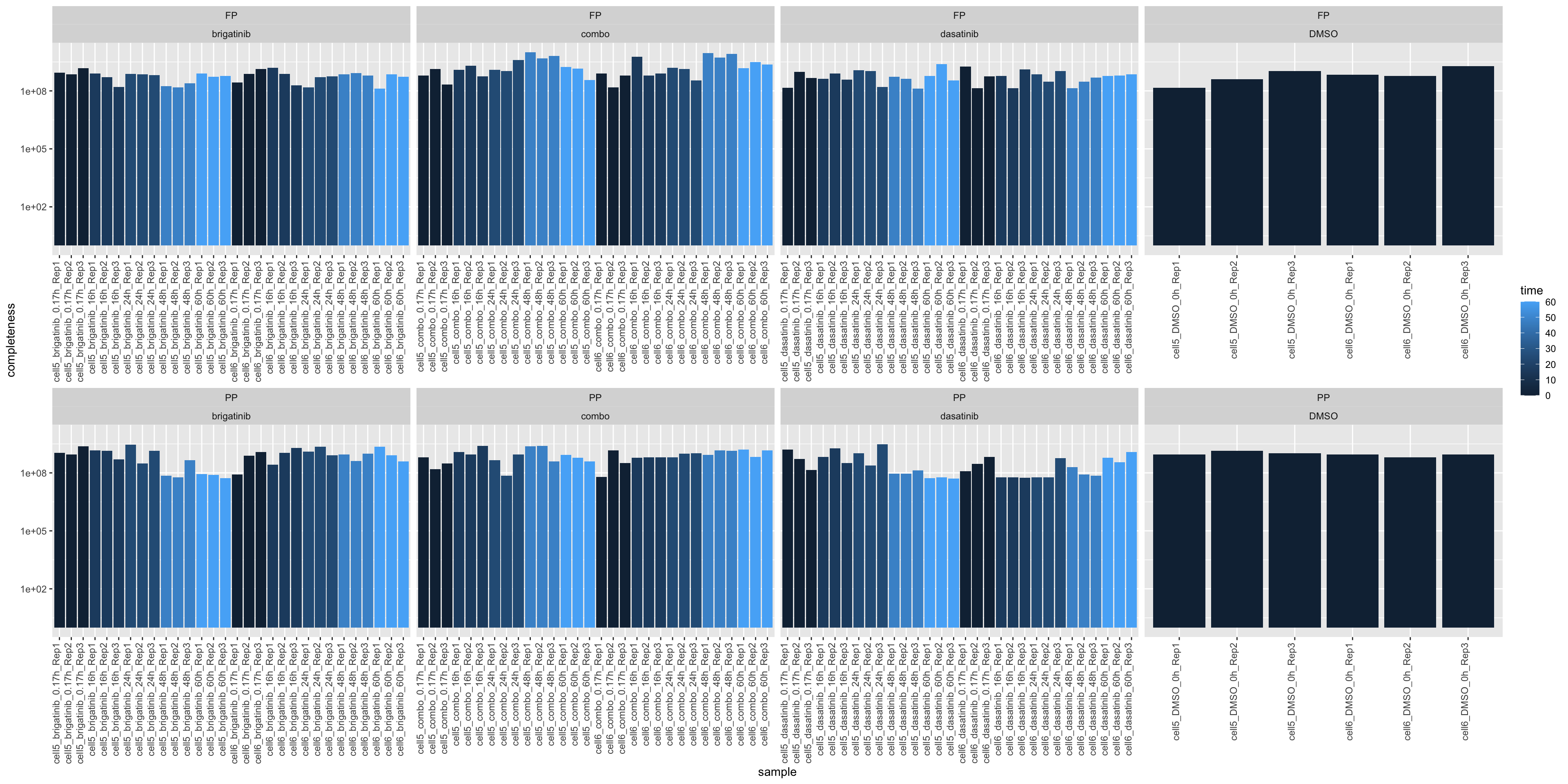
Median Intensity
ggplot(plotTab, aes(x=sample, y=medVal, fill = time)) +
    geom_bar(stat = "identity") +
    ylab("completeness") +
    theme(axis.text.x = element_text(angle = 90, hjust = 1, vjust=0)) +
    facet_wrap(~type+drug, scale = "free_x", ncol=4) +
    scale_y_log10()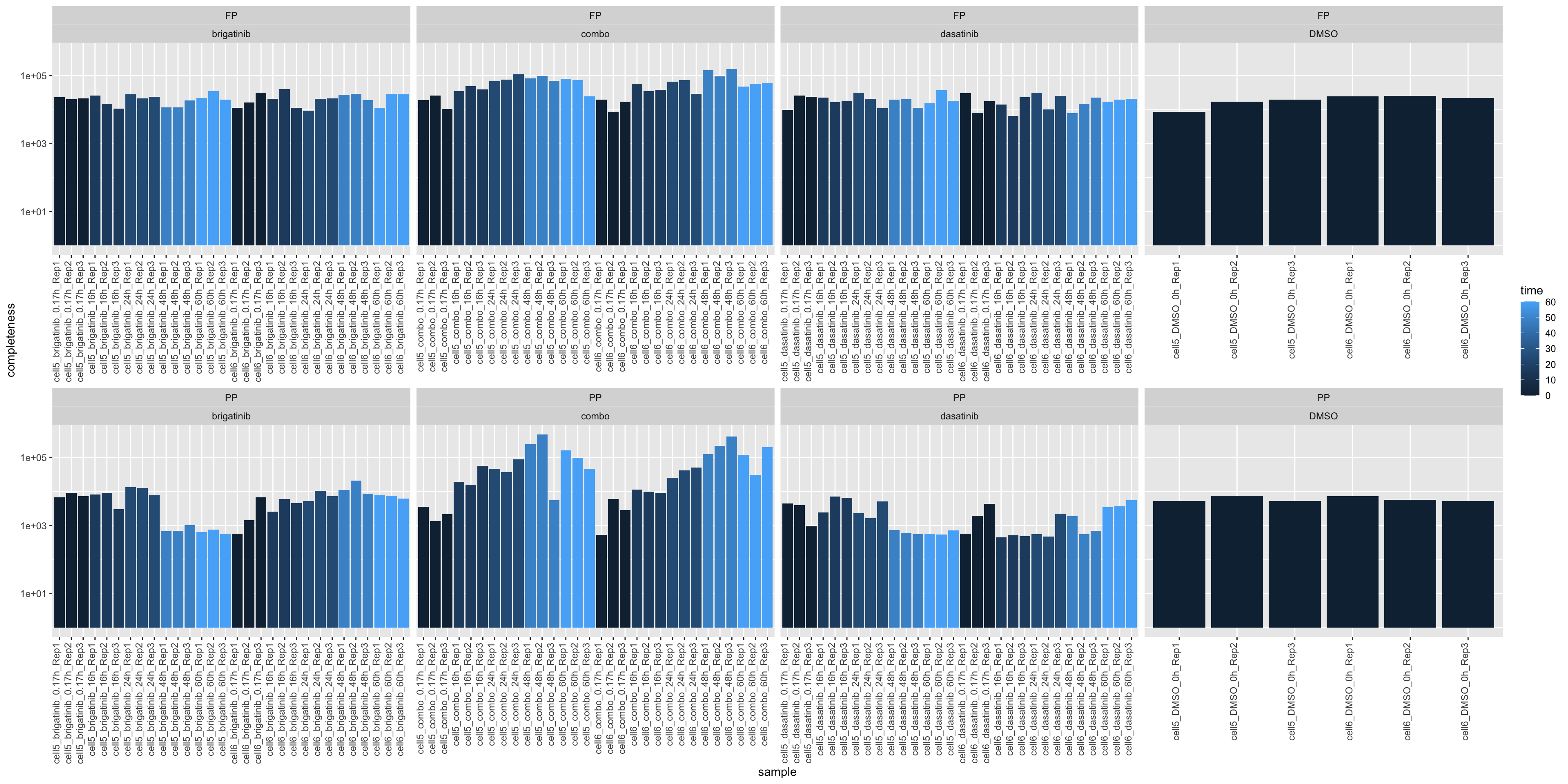
Look at PP sample in the Phosphoproteome experiment
ppePhos <- ppe[,ppe$sampleType != "FP"]
ppePhos <- ppePhos[rowSums(!is.na(assay(ppePhos)))>0,]
dim(ppePhos)
[1] 19853 96How many feature have unique protein mapping?
uniqueVal <- !str_detect(rowData(ppePhos)$Gene,";")
table(uniqueVal)
uniqueVal
FALSE TRUE
225 19628 Missing value per sample
countMat <- assay(ppePhos)
plotTab <- tibble(sample = ppePhos$sample,
                  perNA = colSums(is.na(countMat))/nrow(countMat),
                  time = ppePhos$time,
                  drug = ppePhos$drug)
ggplot(plotTab, aes(x=sample, y=1-perNA)) +
    geom_bar(stat = "identity", aes(fill = time)) +
    ylab("completeness") +
    facet_wrap(~drug, scales = "free_x") +
theme(axis.text.x = element_text(angle = 90, hjust = 1, vjust=0.5)) 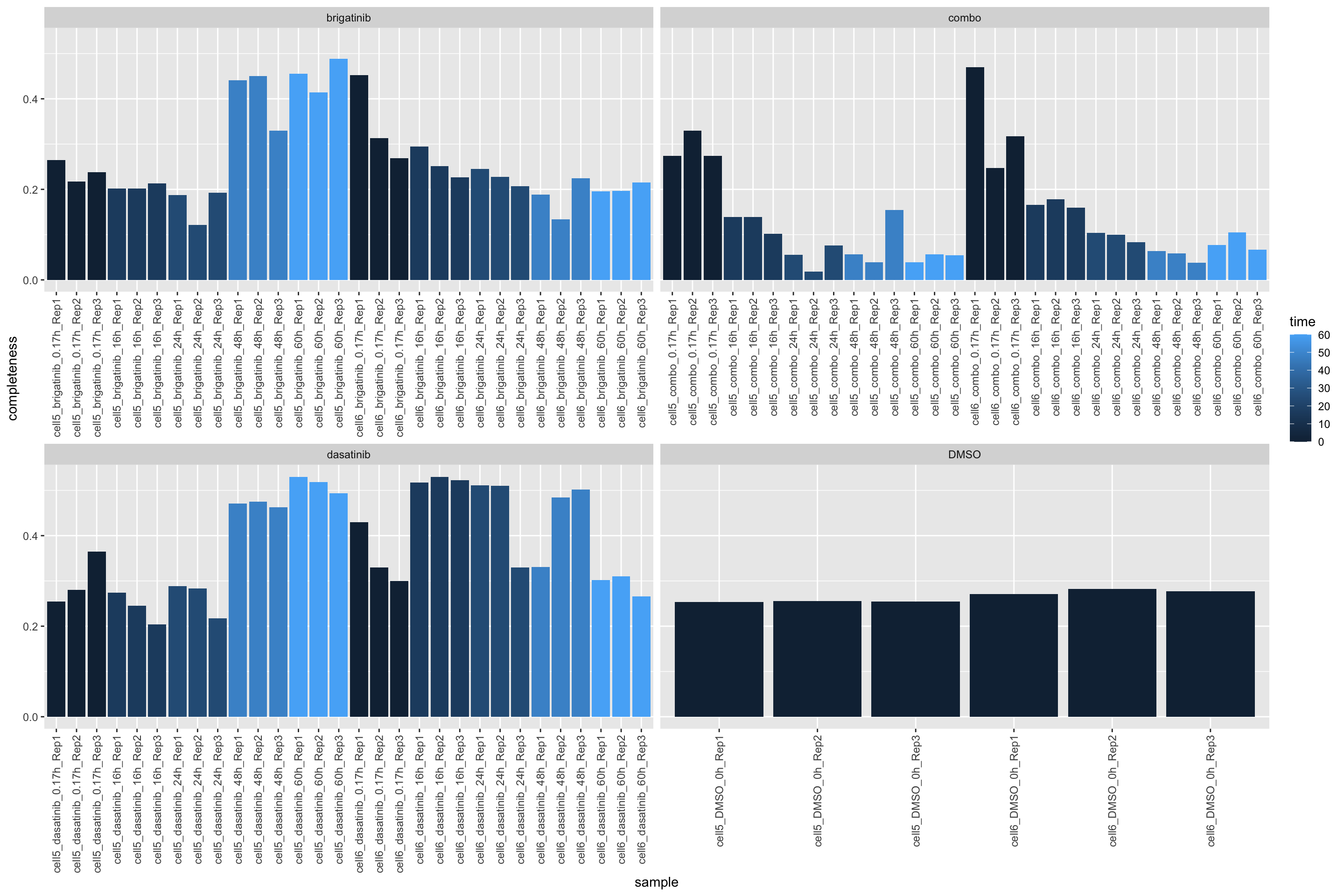
Plot a cumulative curve of missing value cut-off and remaining number of features
missRate <- tibble(id = rownames(countMat),
                   rate = rowSums(is.na(countMat))/ncol(countMat))
cumTab <- lapply(seq(0,1,0.05), function(cutRate) {
    tibble(cut= cutRate,
           per = sum(missRate$rate <= cutRate)/nrow(missRate))
} ) %>%
    bind_rows()
ggplot(cumTab, aes(x=cut,y=per)) +
    geom_line() +
    xlab("Allowed missing value rate") +
    ylab("Percentage of remaining features")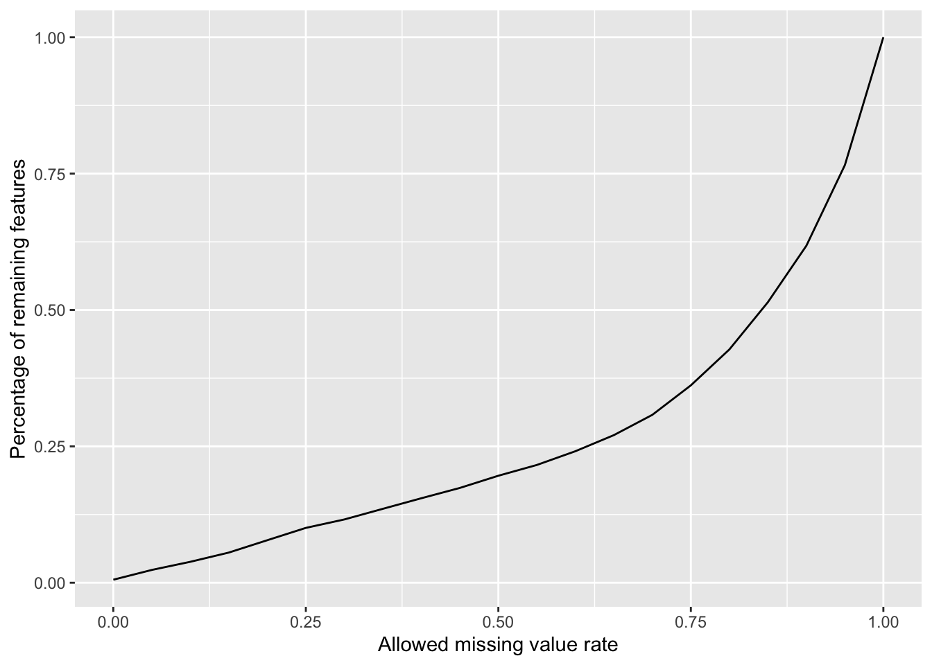
Missing value heatmap to check missing value structure (sample 1000 sites)
DEP::plot_missval(ppePhos[sample(seq(nrow(ppePhos)),1000),])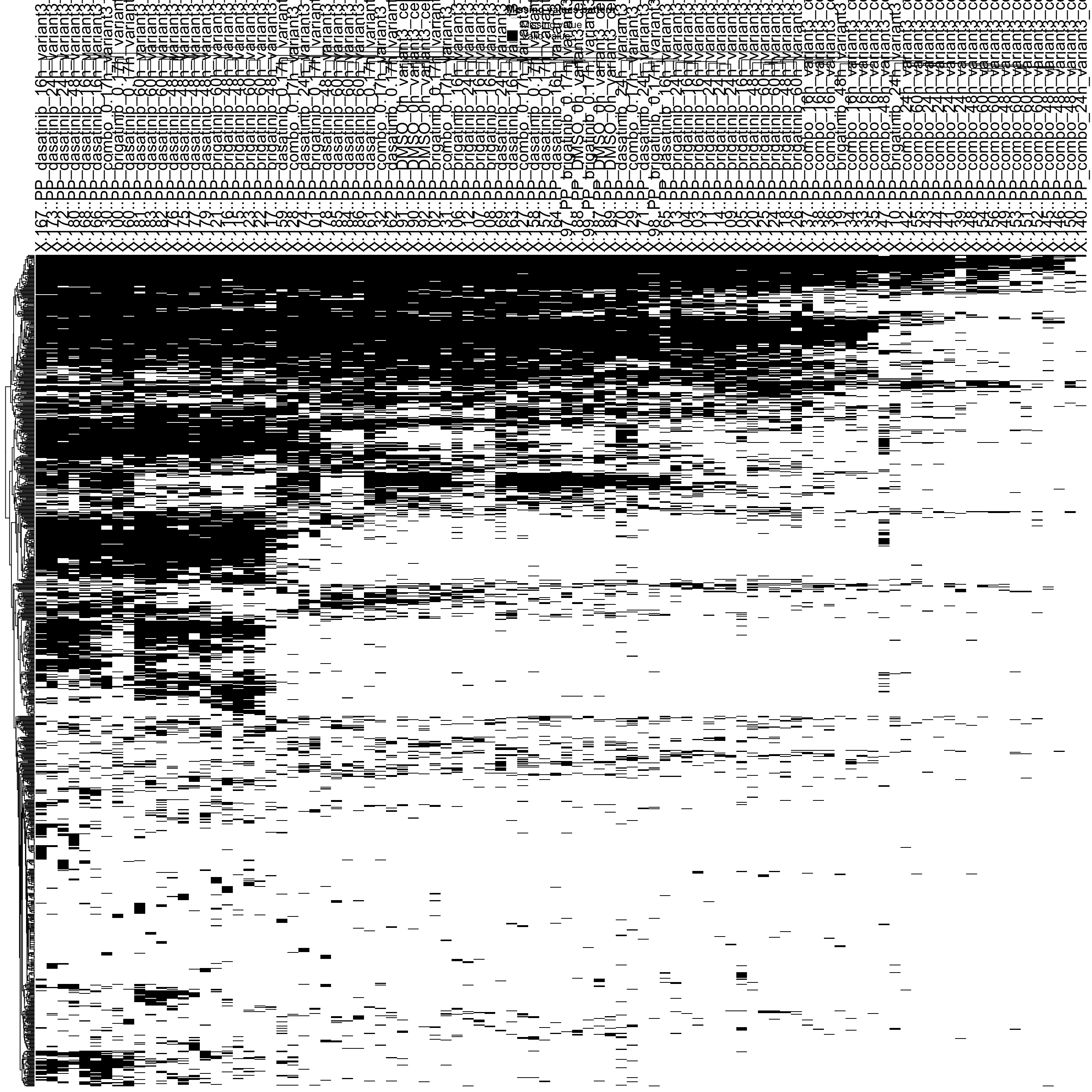
Rather random
Missing value pattern
ppeLog2 <- ppePhos
assay(ppeLog2) <- log2(assay(ppeLog2))
plot_detect(ppeLog2) 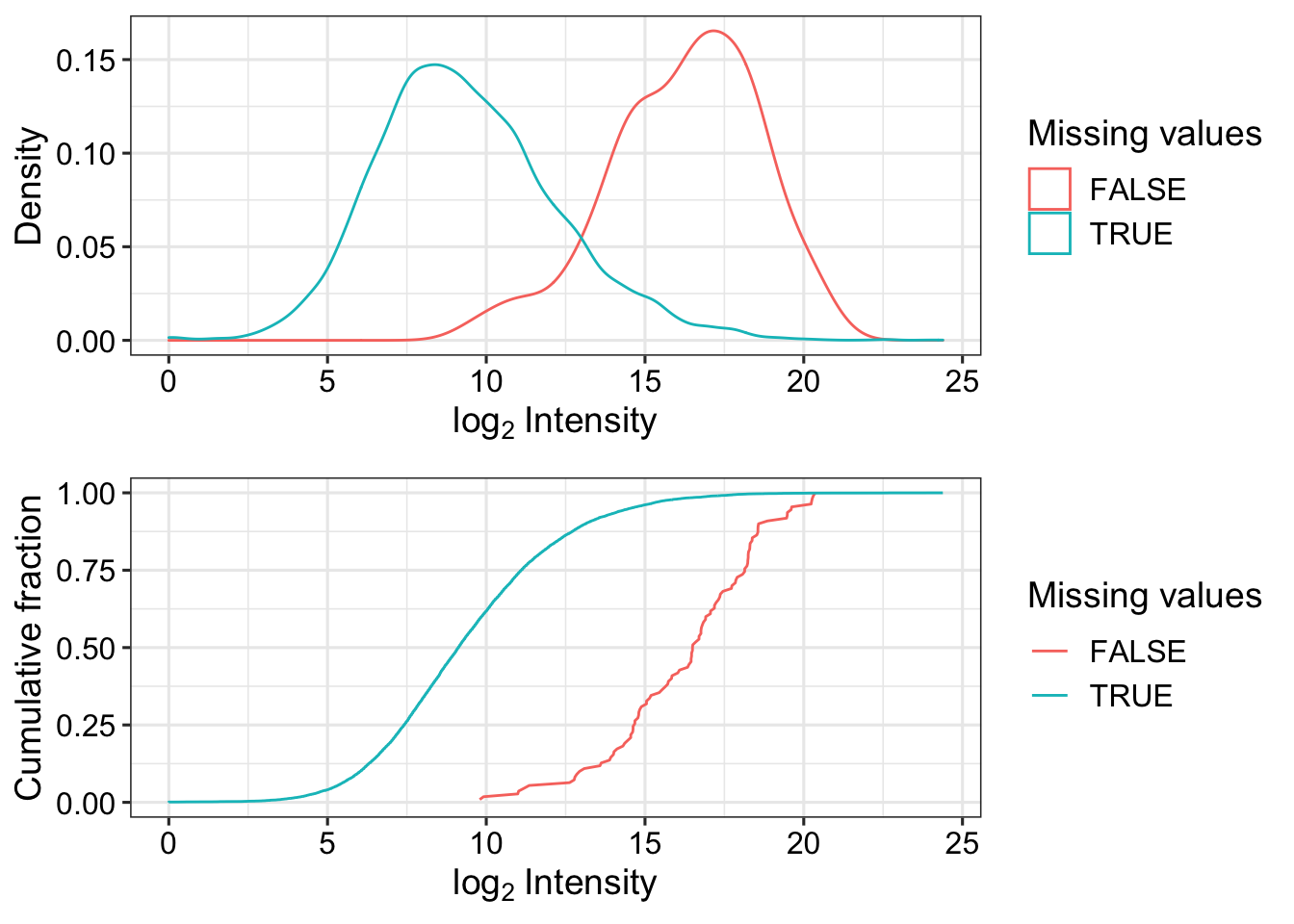
Look at count table distribution
countMat <- assay(ppePhos)
colnames(countMat) <- ppePhos$sample
annoTab <- colData(ppePhos)[,c("sample","time","drug")] %>% as_tibble()
countTab <- countMat %>% as_tibble(rownames = "id") %>%
    pivot_longer(-id) %>%
    filter(!is.na(value)) %>%
    mutate(log2Val = log2(value)) %>%
    left_join(annoTab, by = c(name = "sample"))
ggplot(countTab, aes(x=name, y=log2Val)) +
geom_boxplot(aes(fill = time)) +
facet_wrap(~drug, scales = "free_x") +
theme(axis.text.x = element_text(angle = 90, hjust = 1, vjust = 0.5))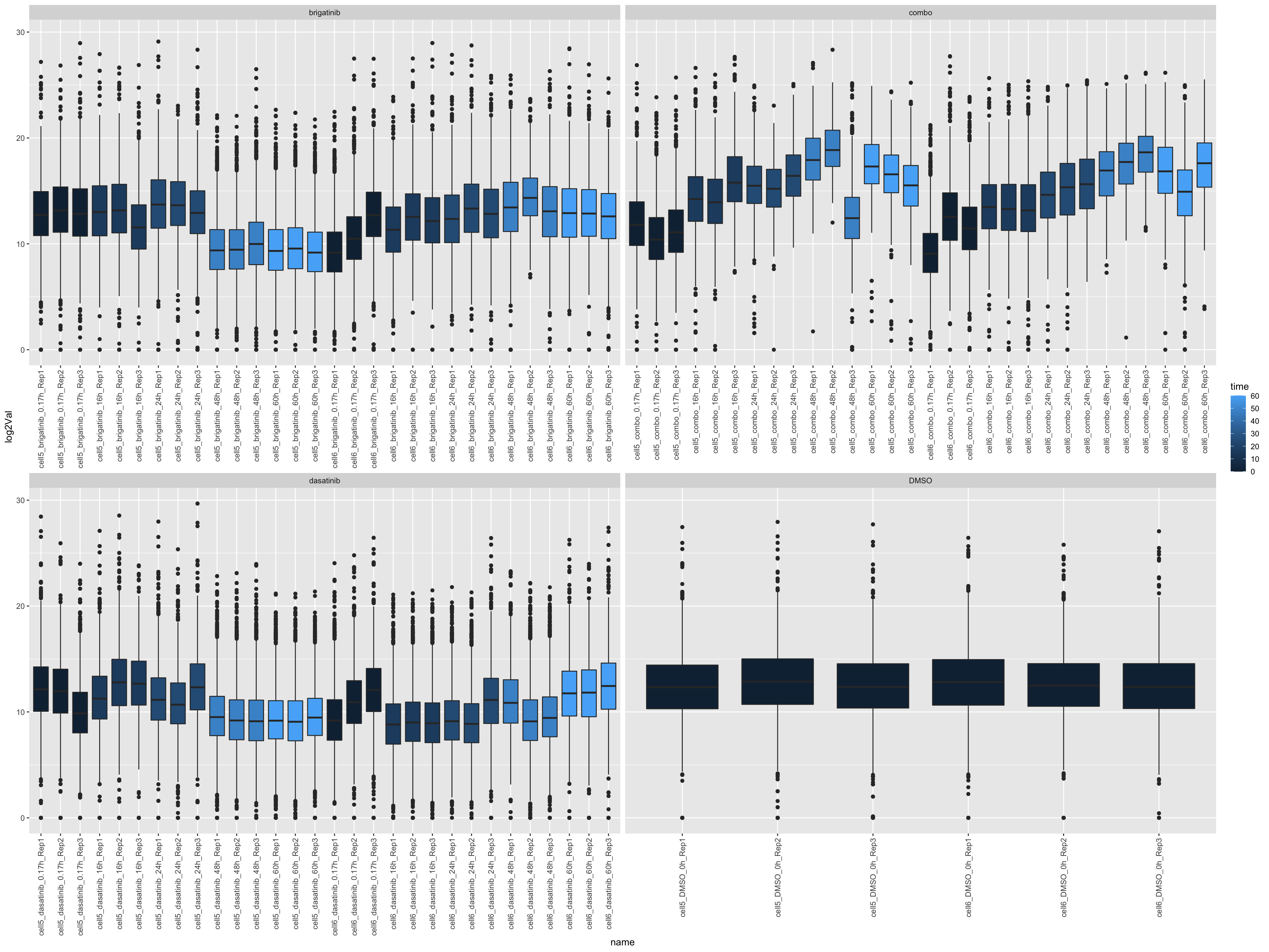
Mean versus variant
logMat <- log2(countMat)
plotTab <- tibble(meanVal = rowMeans(logMat, na.rm = TRUE),
                  var = apply(logMat, 1, var, na.rm=TRUE))
ggplot(plotTab, aes(x=meanVal,y=var)) +
    geom_point() +
    geom_smooth(color = "red")
`geom_smooth()` using method = 'gam' and formula 'y ~ s(x, bs = "cs")'Warning: Removed 1770 rows containing non-finite values (stat_smooth).Warning: Removed 1770 rows containing missing values (geom_point).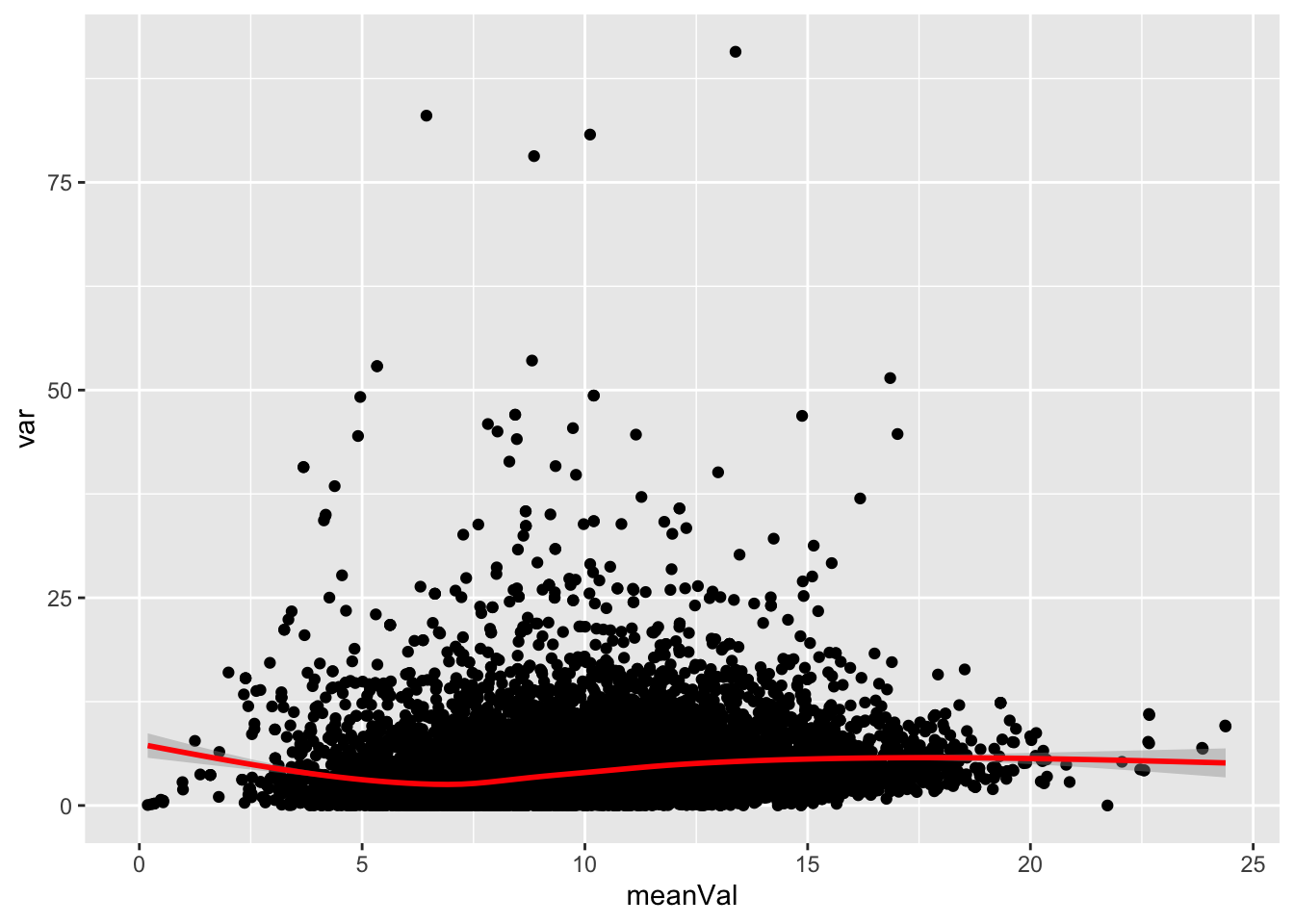
Look at FP sample in the Phosphoproteome experiment
ppePhos <- ppe[,ppe$sampleType != "PP"]
ppePhos <- ppePhos[rowSums(!is.na(assay(ppePhos)))>0,]
dim(ppePhos)
[1] 8029 96How many feature have unique protein mapping?
uniqueVal <- !str_detect(rowData(ppePhos)$Gene,";")
table(uniqueVal)
uniqueVal
FALSE TRUE
102 7927 Missing value per sample
countMat <- assay(ppePhos)
plotTab <- tibble(sample = ppePhos$sample,
                  perNA = colSums(is.na(countMat))/nrow(countMat),
                  time = ppePhos$time,
                  drug = ppePhos$drug)
ggplot(plotTab, aes(x=sample, y=1-perNA)) +
    geom_bar(stat = "identity", aes(fill = time)) +
    ylab("completeness") +
    facet_wrap(~drug, scales = "free_x") +
theme(axis.text.x = element_text(angle = 90, hjust = 1, vjust=0.5)) 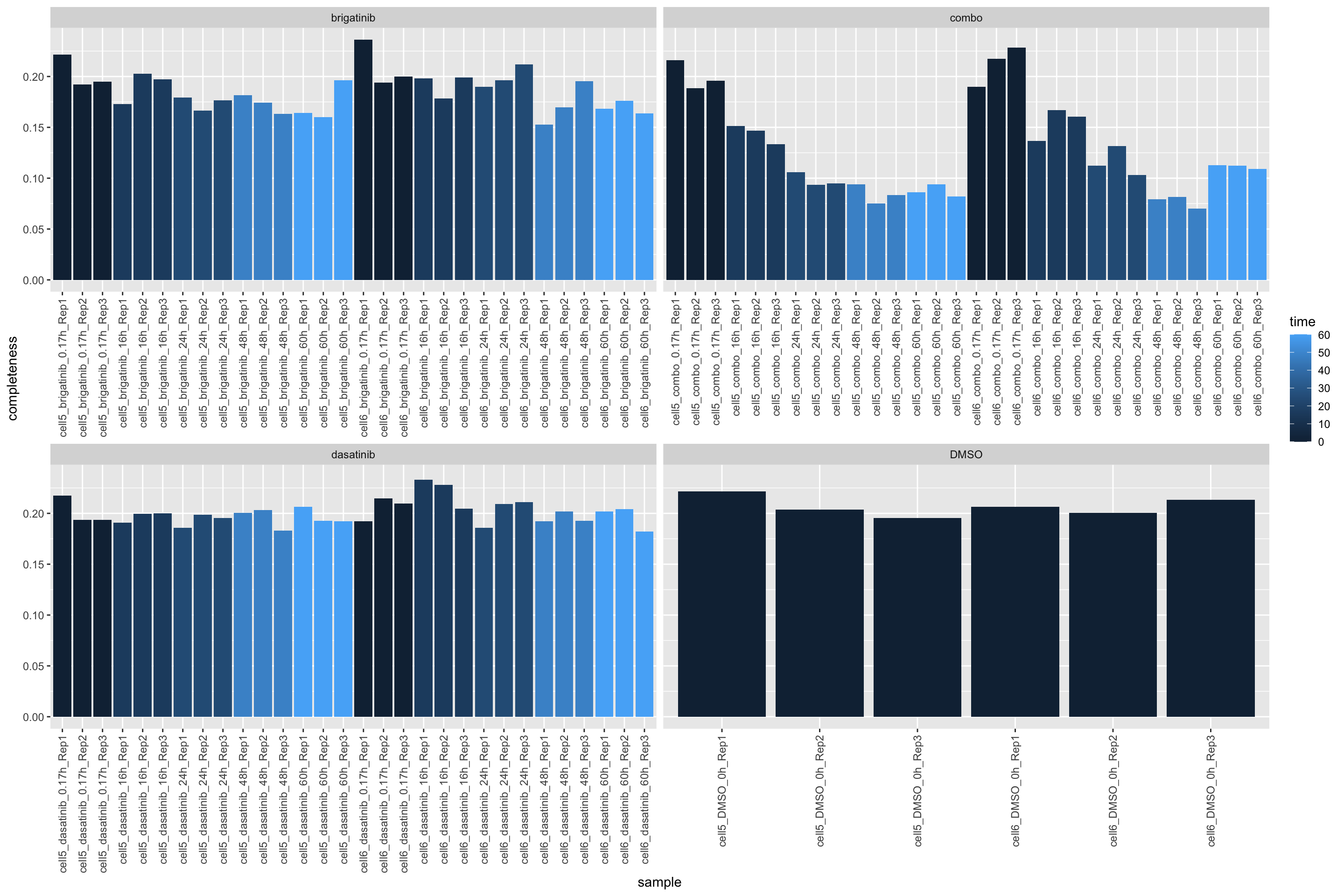
Plot a cumulative curve of missing value cut-off and remaining number of features
missRate <- tibble(id = rownames(countMat),
                   rate = rowSums(is.na(countMat))/ncol(countMat))
cumTab <- lapply(seq(0,1,0.05), function(cutRate) {
    tibble(cut= cutRate,
           per = sum(missRate$rate <= cutRate)/nrow(missRate))
} ) %>%
    bind_rows()
ggplot(cumTab, aes(x=cut,y=per)) +
    geom_line() +
    xlab("Allowed missing value rate") +
    ylab("Percentage of remaining features")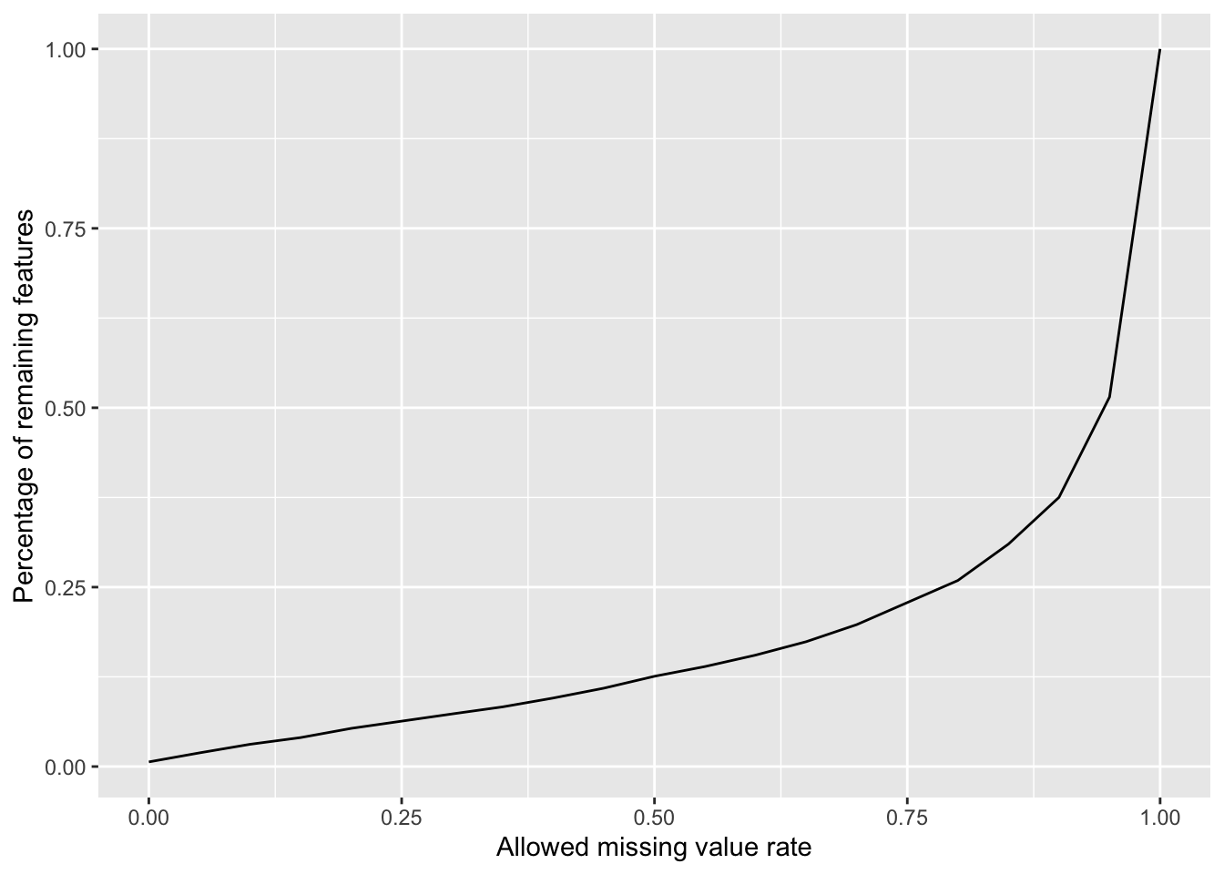
Missing value heatmap to check missing value structure (sample 1000 sites)
DEP::plot_missval(ppePhos[sample(seq(nrow(ppePhos)),1000),])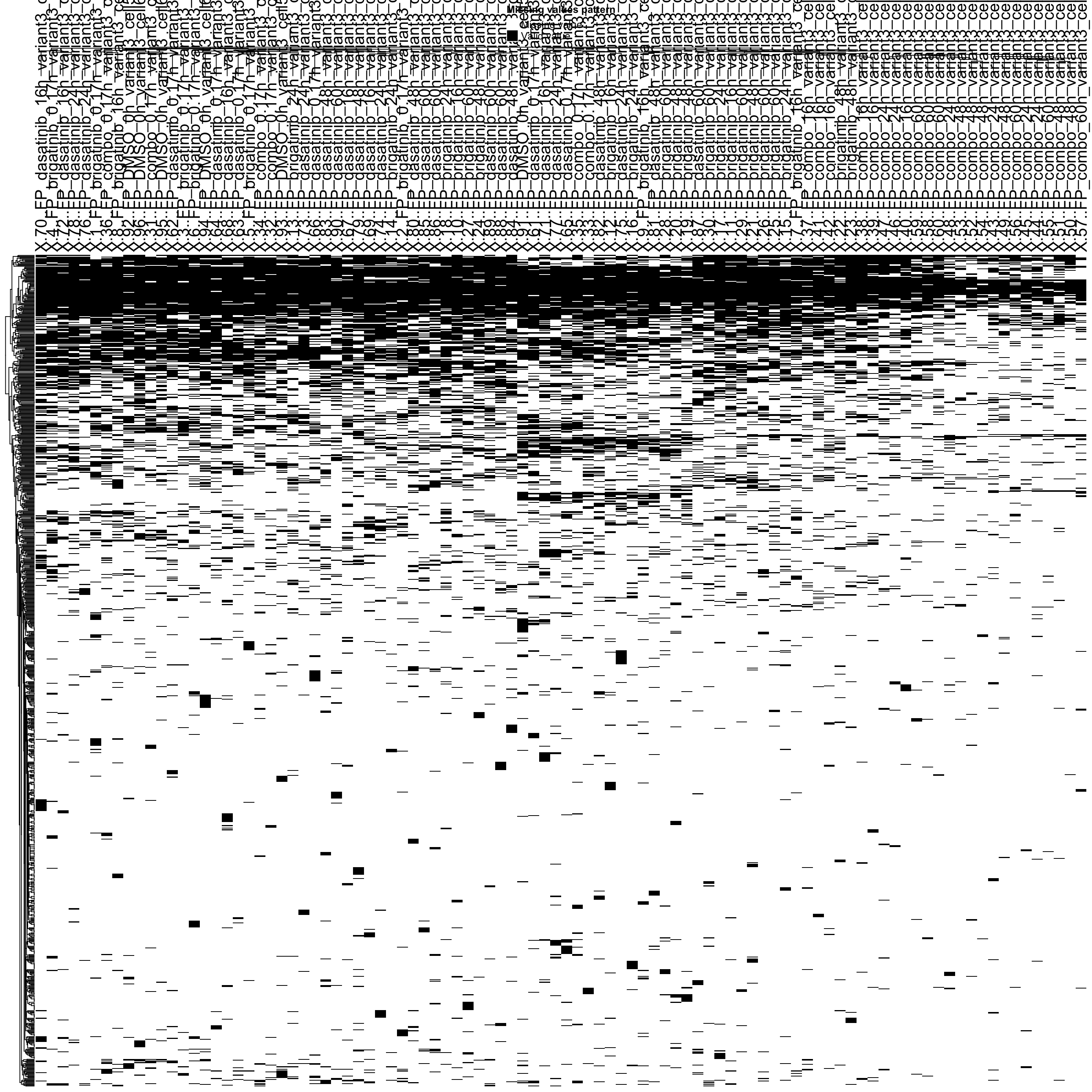
Rather random
Missing value pattern
ppeLog2 <- ppePhos
assay(ppeLog2) <- log2(assay(ppeLog2))
plot_detect(ppeLog2) 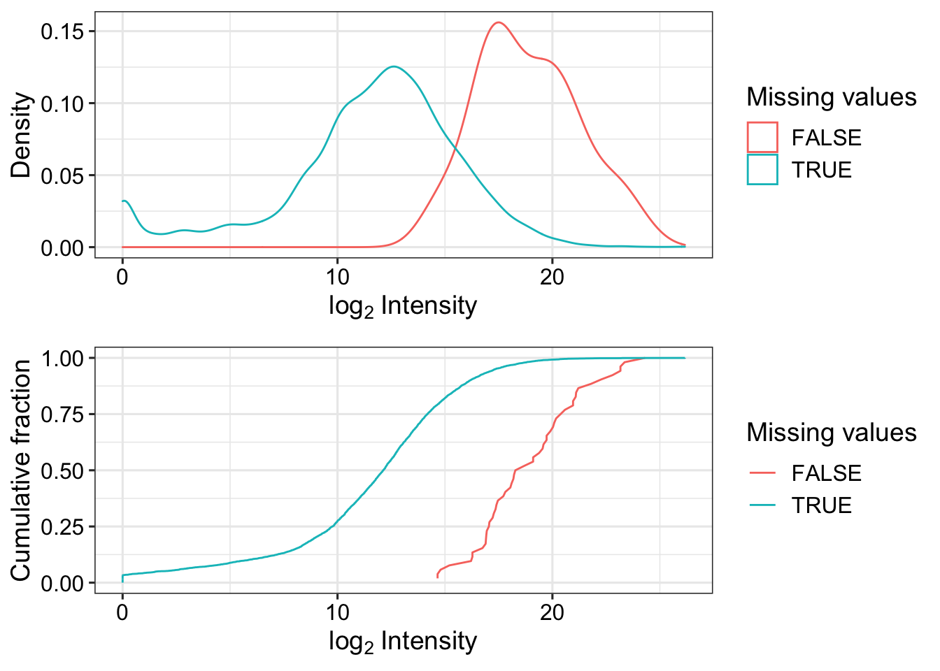
Look at count table distribution
countMat <- assay(ppePhos)
colnames(countMat) <- ppePhos$sample
annoTab <- colData(ppePhos)[,c("sample","time","drug")] %>% as_tibble()
countTab <- countMat %>% as_tibble(rownames = "id") %>%
    pivot_longer(-id) %>%
    filter(!is.na(value)) %>%
    mutate(log2Val = log2(value)) %>%
    left_join(annoTab, by = c(name = "sample"))
ggplot(countTab, aes(x=name, y=log2Val)) +
geom_boxplot(aes(fill = time)) +
facet_wrap(~drug, scales = "free_x") +
theme(axis.text.x = element_text(angle = 90, hjust = 1, vjust = 0.5))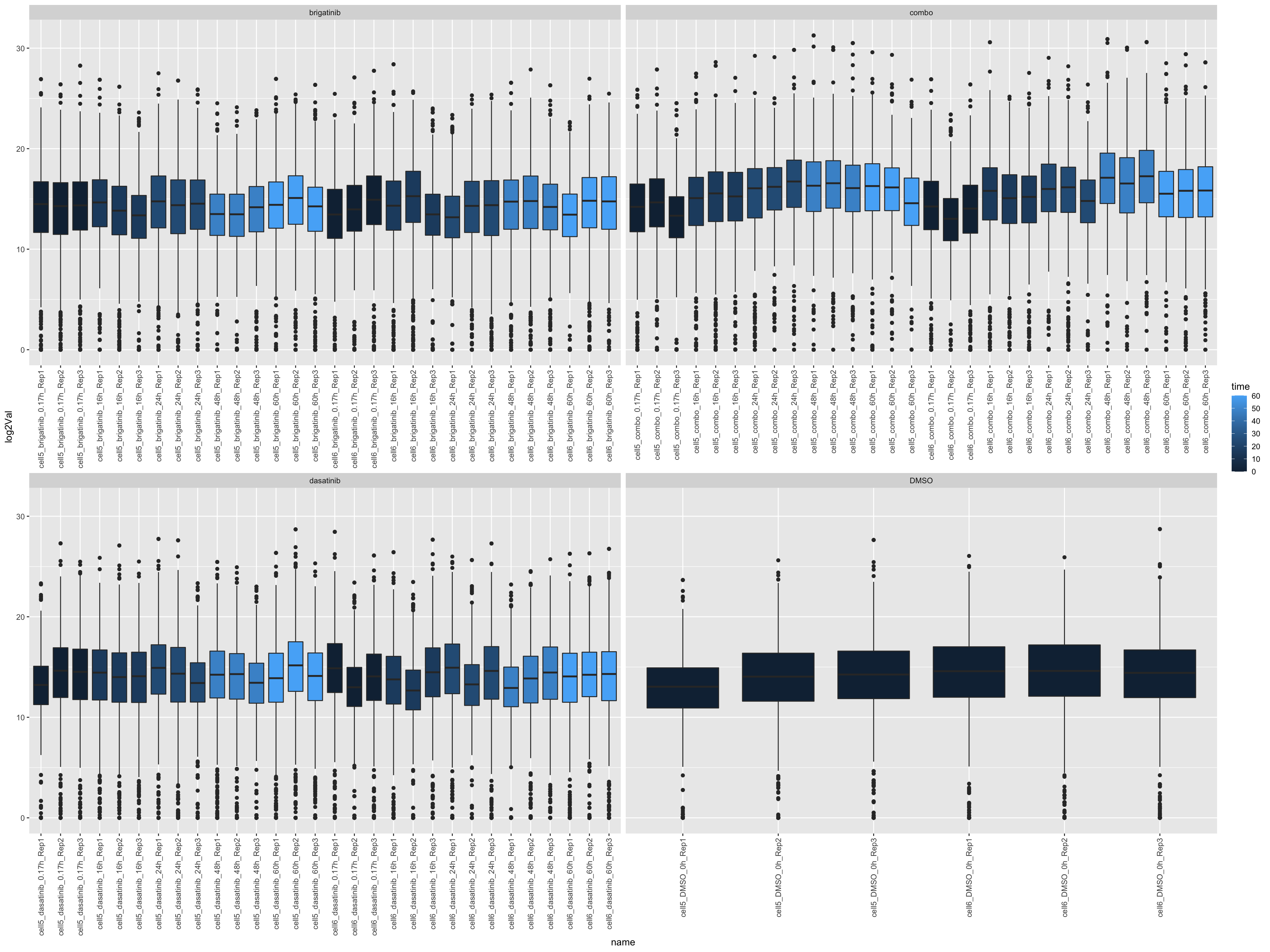
Mean versus variant
logMat <- log2(countMat)
plotTab <- tibble(meanVal = rowMeans(logMat, na.rm = TRUE),
                  var = apply(logMat, 1, var, na.rm=TRUE))
ggplot(plotTab, aes(x=meanVal,y=var)) +
    geom_point() +
    geom_smooth(color = "red")
`geom_smooth()` using method = 'gam' and formula 'y ~ s(x, bs = "cs")'Warning: Removed 1913 rows containing non-finite values (stat_smooth).Warning: Removed 1913 rows containing missing values (geom_point).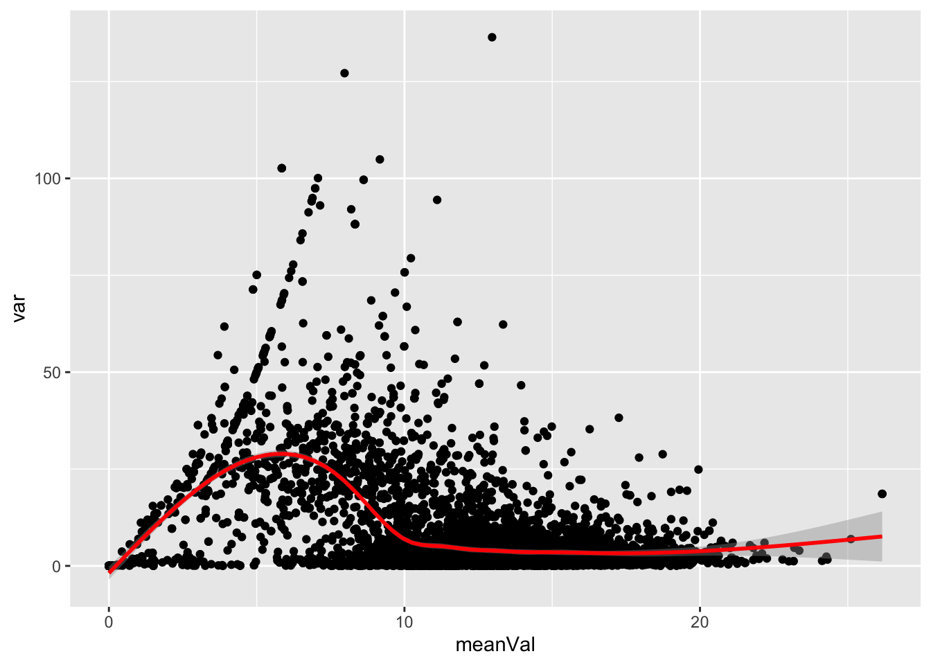
Check full proteome measurement
Subset for full proteome data
fpe <- maeData[["Proteome"]]
colData(fpe) <- colData(maeData)
Examin the data distrubution
countMat <- assay(fpe)Missing value per sample
plotTab <- tibble(sample = fpe$sample,
                  perNA = colSums(is.na(countMat))/nrow(countMat),
                  total = colSums(countMat, na.rm=TRUE),
                  medVal = colMedians(countMat, na.rm=TRUE),
                  type = fpe$sampleType,
                  time = fpe$time,
                  drug = fpe$drug)
ggplot(plotTab, aes(x=sample, y=1-perNA, fill = time)) +
    geom_bar(stat = "identity") +
    ylab("completeness") +
    theme(axis.text.x = element_text(angle = 90, hjust = 1, vjust=0)) +
    facet_wrap(~type+drug, scale = "free_x", ncol=4)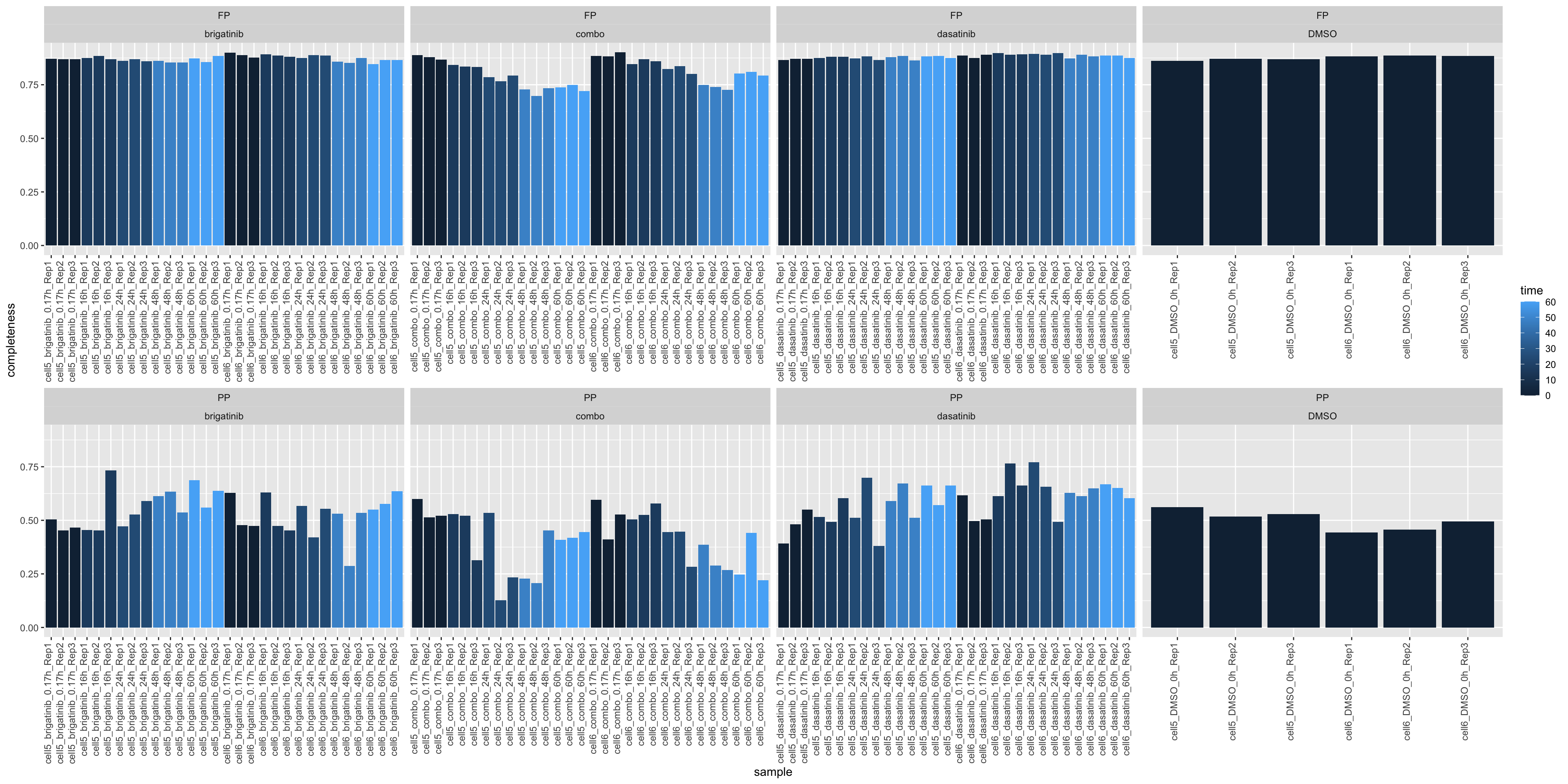
Total intensity
ggplot(plotTab, aes(x=sample, y=total, fill = time)) +
    geom_bar(stat = "identity") +
    ylab("completeness") +
    theme(axis.text.x = element_text(angle = 90, hjust = 1, vjust=0)) +
    facet_wrap(~type+drug, scale = "free_x", ncol=4) +
    scale_y_log10()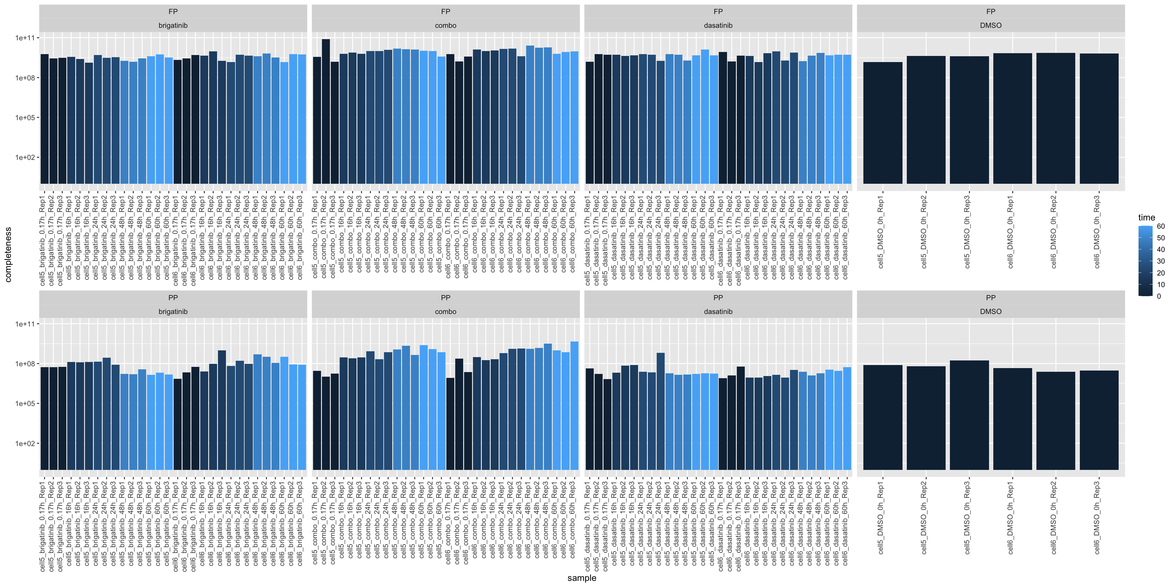
Median Intensity
ggplot(plotTab, aes(x=sample, y=medVal, fill = time)) +
    geom_bar(stat = "identity") +
    ylab("completeness") +
    theme(axis.text.x = element_text(angle = 90, hjust = 1, vjust=0)) +
    facet_wrap(~type+drug, scale = "free_x", ncol=4) +
    scale_y_log10()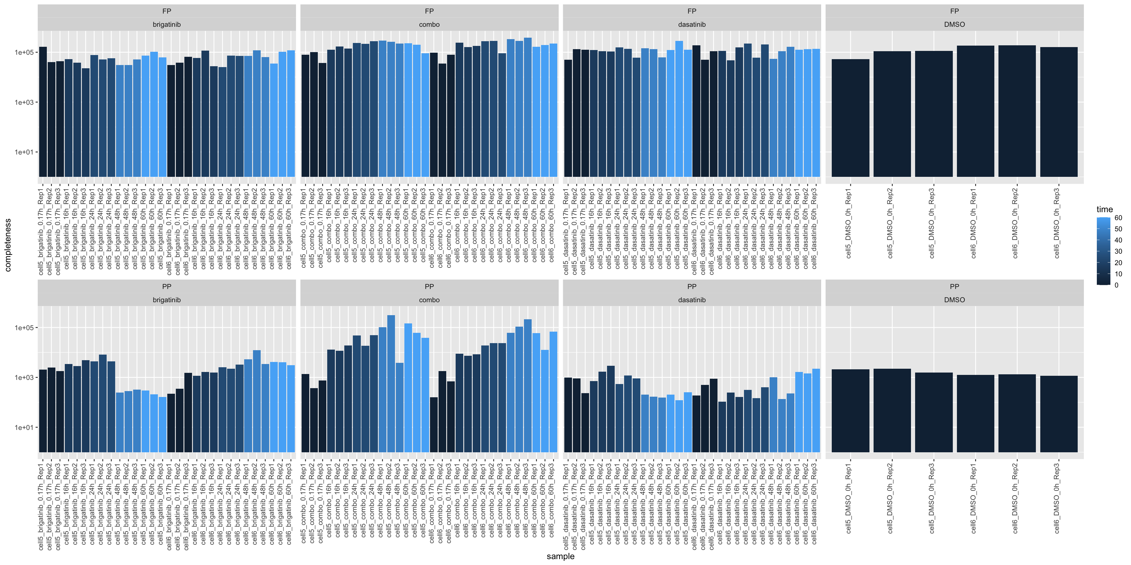
Missing value heatmap to check missing value structure
DEP::plot_missval(fpe[sample(seq(nrow(fpe)),1000),])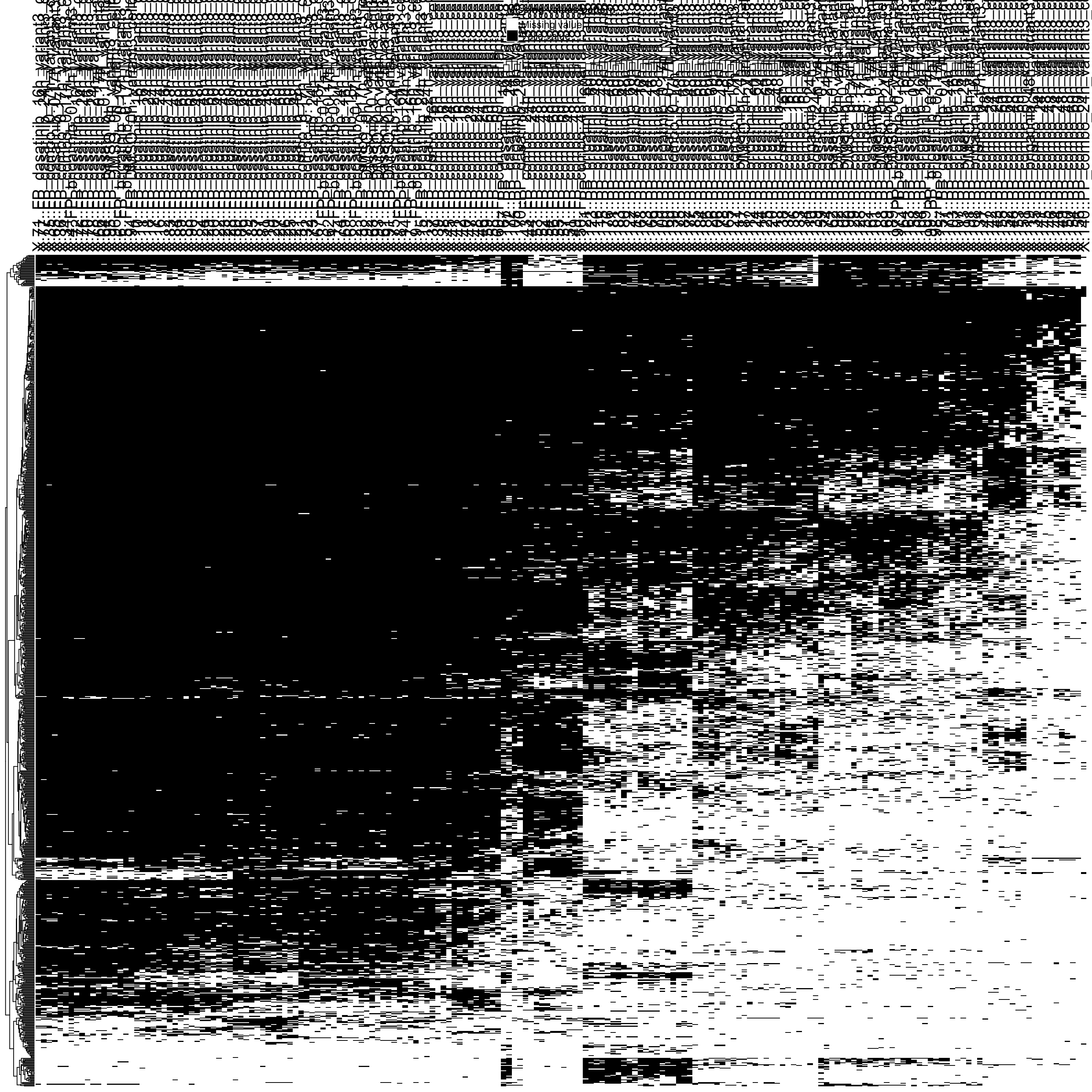
Look at FP samples only
fpeProt <- fpe[,fpe$sampleType == "FP"]
fpeProt <- fpeProt[rowSums(!is.na(assay(fpeProt)))>0,]
countMat <- assay(fpeProt)
dim(fpeProt)
[1] 8384 96How many feature have unique protein mapping?
uniqueVal <- !str_detect(rowData(fpeProt)$Gene,";")
table(uniqueVal)
uniqueVal
FALSE TRUE
104 8280 Plot a cumulative curve of missing value cut-off and remaining number of features
missRate <- tibble(id = rownames(countMat),
                   rate = rowSums(is.na(countMat))/ncol(countMat))
cumTab <- lapply(seq(0,1,0.05), function(cutRate) {
    tibble(cut= cutRate,
           per = sum(missRate$rate <= cutRate)/nrow(missRate))
} ) %>%
    bind_rows()
ggplot(cumTab, aes(x=cut,y=per)) +
    geom_line() +
    xlab("Allowed missing value rate") +
    ylab("Percentage of remaining features")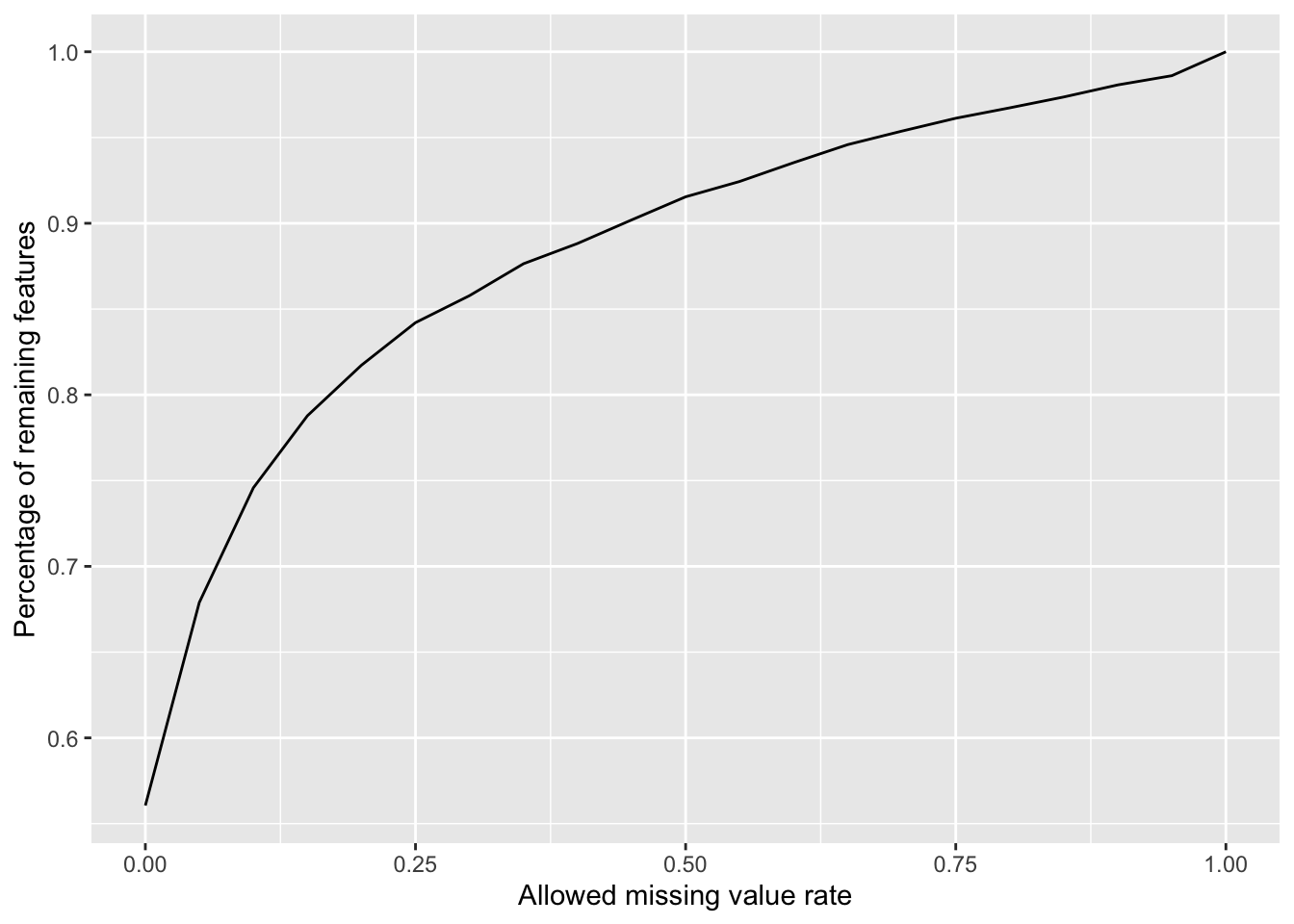
Missing value pattern
fpeLog2 <- fpeProt
assay(fpeLog2) <- log2(assay(fpeLog2))
plot_detect(fpeLog2) 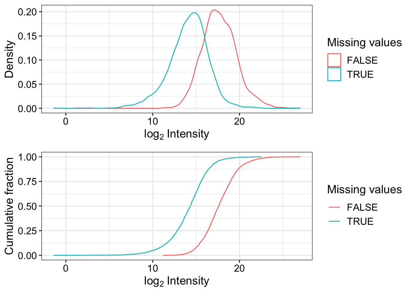
countMat <- assay(fpeProt)
colnames(countMat) <- fpeProt$sample
annoTab <- colData(fpeProt)[,c("sample","time","drug")] %>% as_tibble()
countTab <- countMat %>% as_tibble(rownames = "id") %>%
    pivot_longer(-id) %>%
    filter(!is.na(value)) %>%
    mutate(log2Val = log2(value)) %>%
    left_join(annoTab, by = c(name = "sample"))
ggplot(countTab, aes(x=name, y=log2Val)) +
geom_boxplot(aes(fill = time)) +
facet_wrap(~drug, scales = "free_x") +
theme(axis.text.x = element_text(angle = 90, hjust = 1, vjust = 0.5))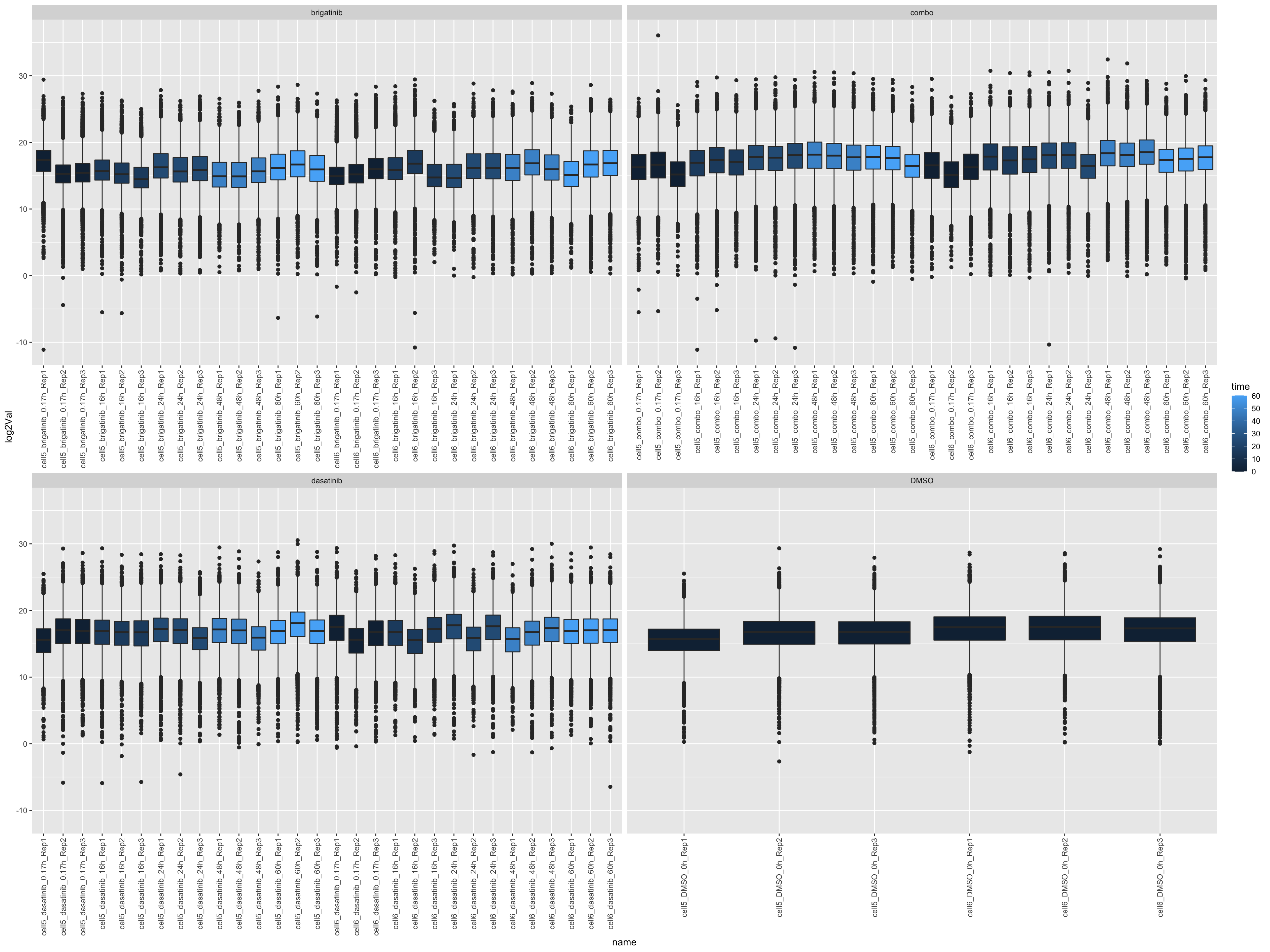
Mean versus variant
logMat <- log2(countMat)
plotTab <- tibble(meanVal = rowMeans(logMat, na.rm = TRUE),
                  var = apply(logMat, 1, var, na.rm=TRUE))
ggplot(plotTab, aes(x=meanVal,y=var)) +
    geom_point() +
    geom_smooth(color = "red")
`geom_smooth()` using method = 'gam' and formula 'y ~ s(x, bs = "cs")'Warning: Removed 52 rows containing non-finite values (stat_smooth).Warning: Removed 52 rows containing missing values (geom_point).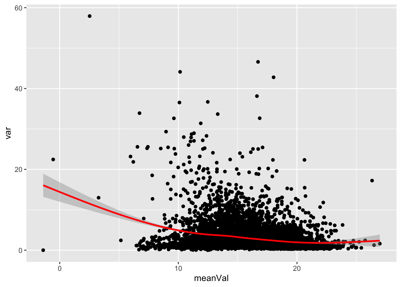
Look at PP samples only
fpeProt <- fpe[,fpe$sampleType == "PP"]
fpeProt <- fpeProt[rowSums(!is.na(assay(fpeProt)))>0,]
countMat <- assay(fpeProt)
dim(fpeProt)
[1] 8262 96How many feature have unique protein mapping?
uniqueVal <- !str_detect(rowData(fpeProt)$Gene,";")
table(uniqueVal)
uniqueVal
FALSE TRUE
100 8162 Plot a cumulative curve of missing value cut-off and remaining number of features
missRate <- tibble(id = rownames(countMat),
                   rate = rowSums(is.na(countMat))/ncol(countMat))
cumTab <- lapply(seq(0,1,0.05), function(cutRate) {
    tibble(cut= cutRate,
           per = sum(missRate$rate <= cutRate)/nrow(missRate))
} ) %>%
    bind_rows()
ggplot(cumTab, aes(x=cut,y=per)) +
    geom_line() +
    xlab("Allowed missing value rate") +
    ylab("Percentage of remaining features")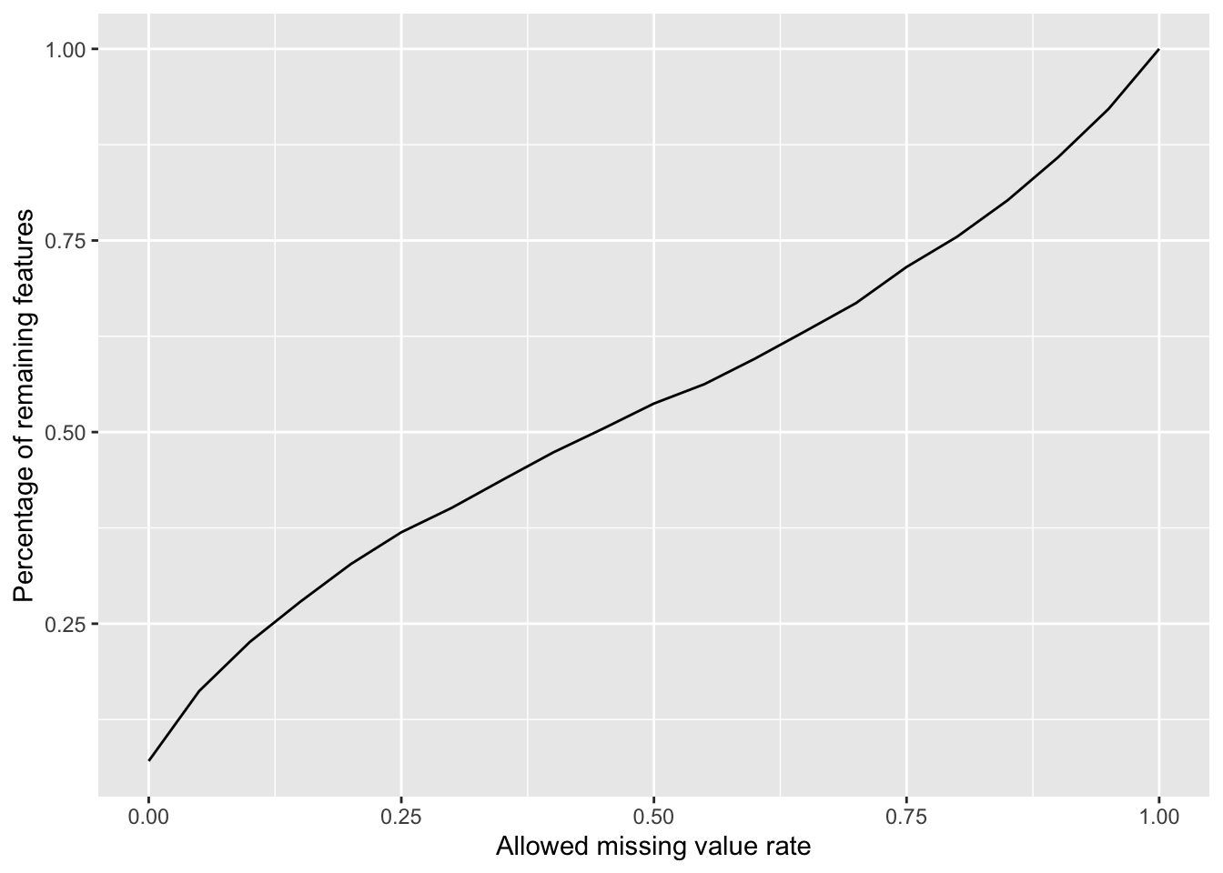
Missing value pattern
fpeLog2 <- fpeProt
assay(fpeLog2) <- log2(assay(fpeLog2))
plot_detect(fpeLog2) 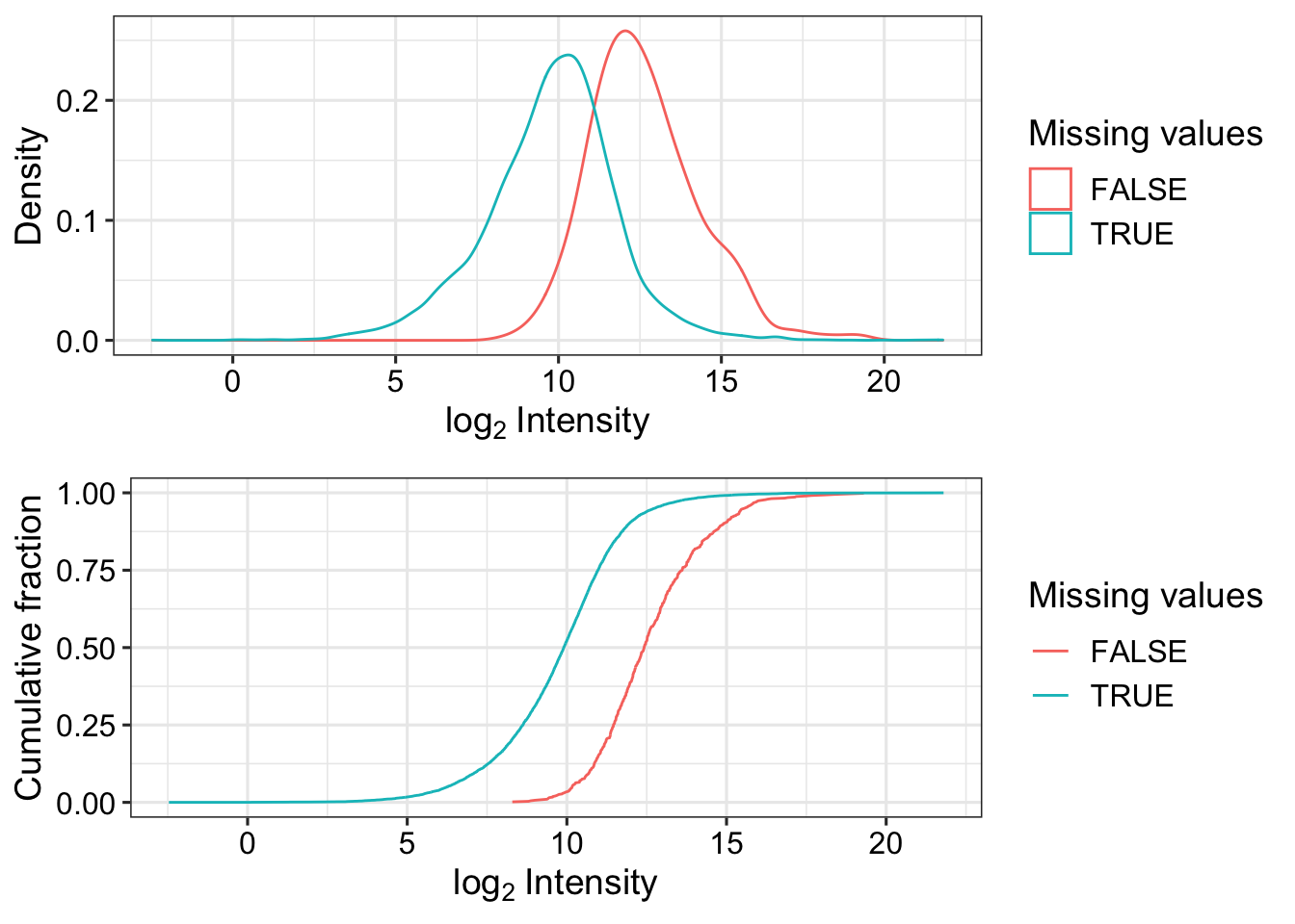
countMat <- assay(fpeProt)
colnames(countMat) <- fpeProt$sample
annoTab <- colData(fpeProt)[,c("sample","time","drug")] %>% as_tibble()
countTab <- countMat %>% as_tibble(rownames = "id") %>%
    pivot_longer(-id) %>%
    filter(!is.na(value)) %>%
    mutate(log2Val = log2(value)) %>%
    left_join(annoTab, by = c(name = "sample"))
ggplot(countTab, aes(x=name, y=log2Val)) +
geom_boxplot(aes(fill = time)) +
facet_wrap(~drug, scales = "free_x") +
theme(axis.text.x = element_text(angle = 90, hjust = 1, vjust = 0.5))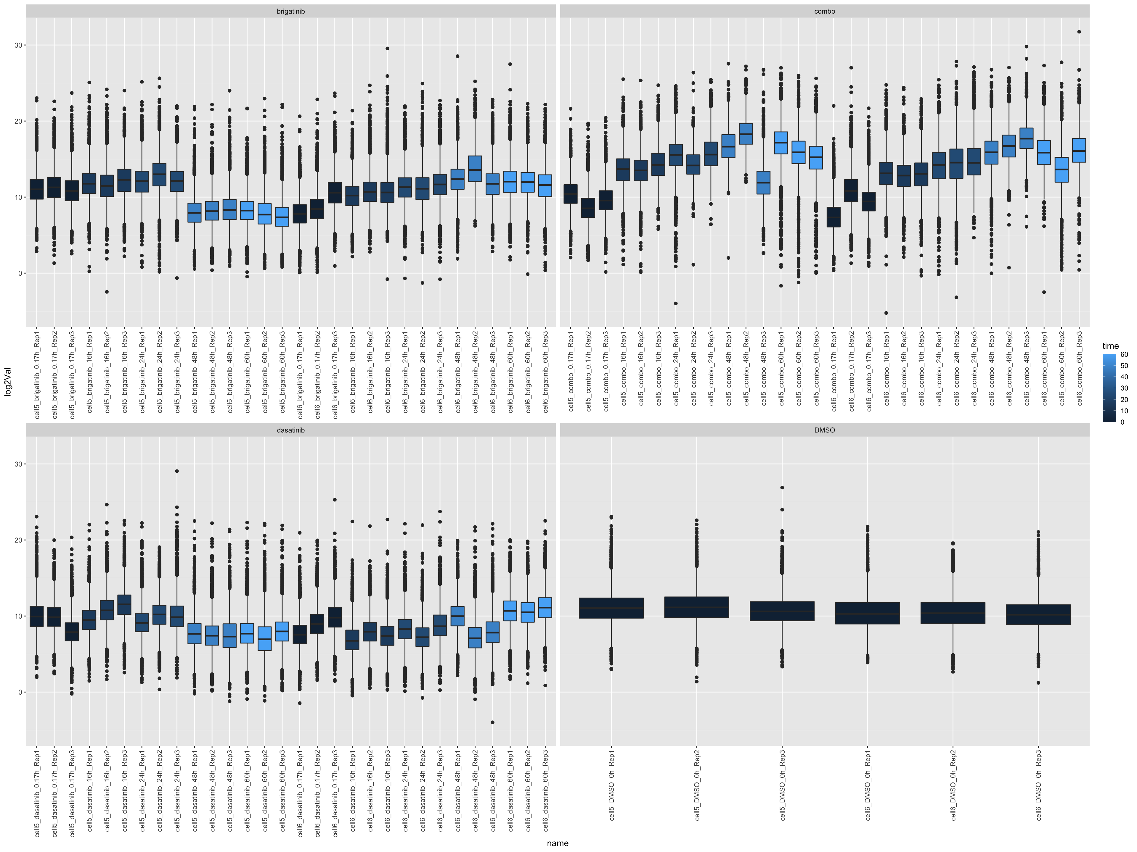
Mean versus variant
logMat <- log2(countMat)
plotTab <- tibble(meanVal = rowMeans(logMat, na.rm = TRUE),
                  var = apply(logMat, 1, var, na.rm=TRUE))
ggplot(plotTab, aes(x=meanVal,y=var)) +
    geom_point() +
    geom_smooth(color = "red")
`geom_smooth()` using method = 'gam' and formula 'y ~ s(x, bs = "cs")'Warning: Removed 209 rows containing non-finite values (stat_smooth).Warning: Removed 209 rows containing missing values (geom_point).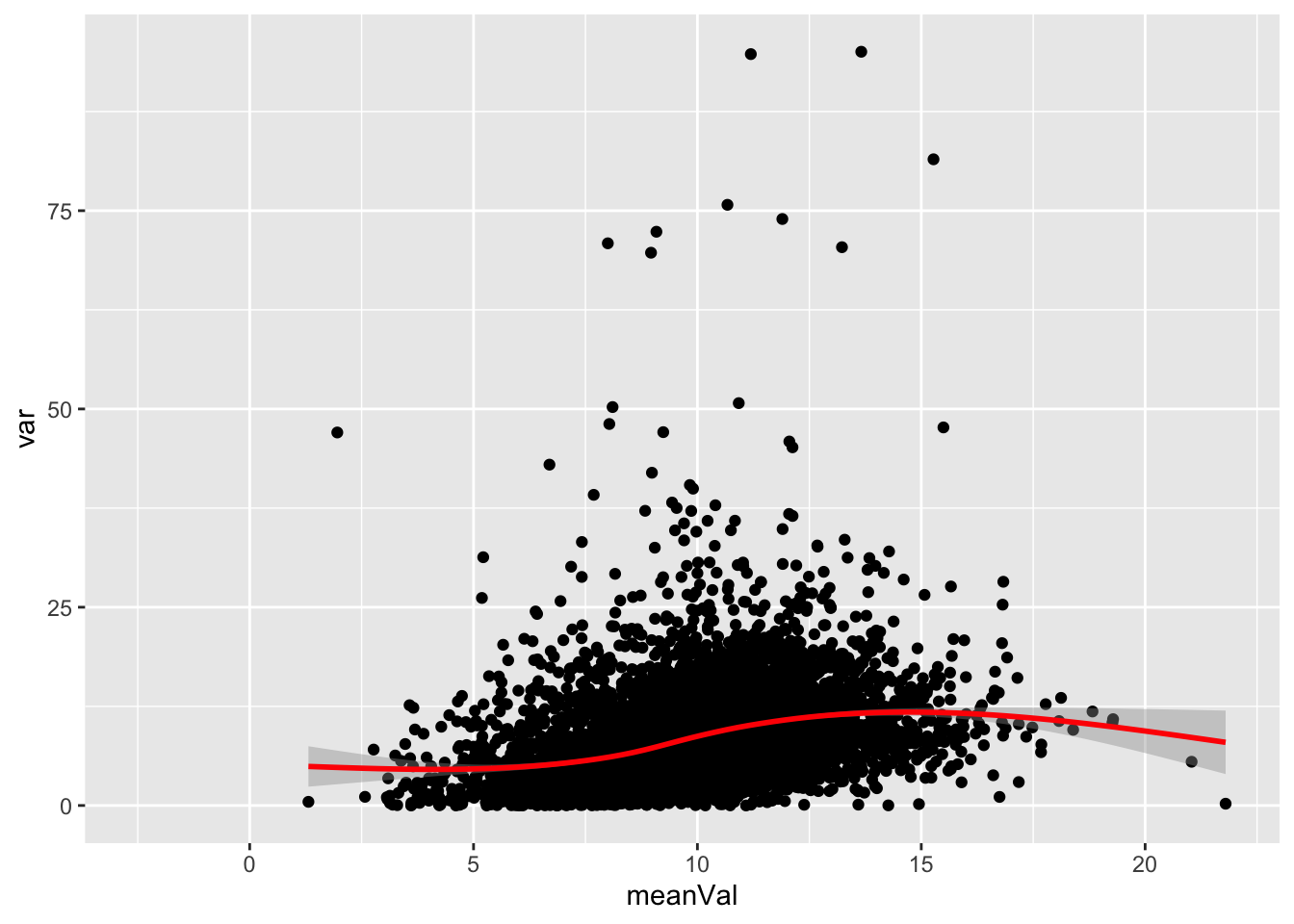
Check precursur distribution
preMat <- read_tsv("../data/20221021_Lung_Mouse_CellLines_Phospho_TimeCourse_SUP_OTEC_SotilloCollab_SN16.2/20221021_065120_20221019_EA_LungTumor_CellLines_Mouse_Phospho_SotilloCollab_SN16.2_Precursor_Report.xls") %>%
  select(EG.PrecursorId, contains("TotalQuantity"))
Rows: 184725 Columns: 389
── Column specification ────────────────────────────────────────────────────────
Delimiter: "\t"
chr (388): PG.ProteinGroups, PEP.StrippedSequence, EG.PrecursorId, EG.Modifi...
lgl (1): EG.IsDecoy
ℹ Use `spec()` to retrieve the full column specification for this data.
ℹ Specify the column types or set `show_col_types = FALSE` to quiet this message.expTab <- preMat %>%
pivot_longer(-EG.PrecursorId) %>%
mutate(value = as.numeric(str_replace(value,",","."))) %>%
filter(!is.na(value)) %>%
mutate(sample = str_extract(name, "(?<= ).+(?=.raw)")) %>%
mutate(sample = str_remove(sample, "_variant3")) %>%
mutate(sampleType = ifelse(str_detect(sample,"FP"),"FP","PP"),
drug = str_extract(sample, "(?<=_).+(?=_\\d)")) %>%
mutate(time = str_extract(sample, "(?<=DMSO_|brigatinib_|combo_|dasatinib_).+(?=h_)")) %>%
mutate(time = as.numeric(str_replace(time,",",".")))Warning in mask$eval_all_mutate(quo): NAs introduced by coercionSummarisation
sumTab <- group_by(expTab, sample, sampleType, drug, time) %>%
  summarise(medVal = median(value),
            total = sum(value),
            num = length(EG.PrecursorId))
`summarise()` has grouped output by 'sample', 'sampleType', 'drug'. You can
override using the `.groups` argument.Summarise total counts
Number of identification
ggplot(sumTab, aes(x=sample, y=num, fill = time)) +
    geom_bar(stat = "identity") +
    ylab("completeness") +
    theme(axis.text.x = element_text(angle = 90, hjust = 1, vjust=0)) +
    facet_wrap(~sampleType+drug, scale = "free_x", ncol=4) +
    scale_y_log10()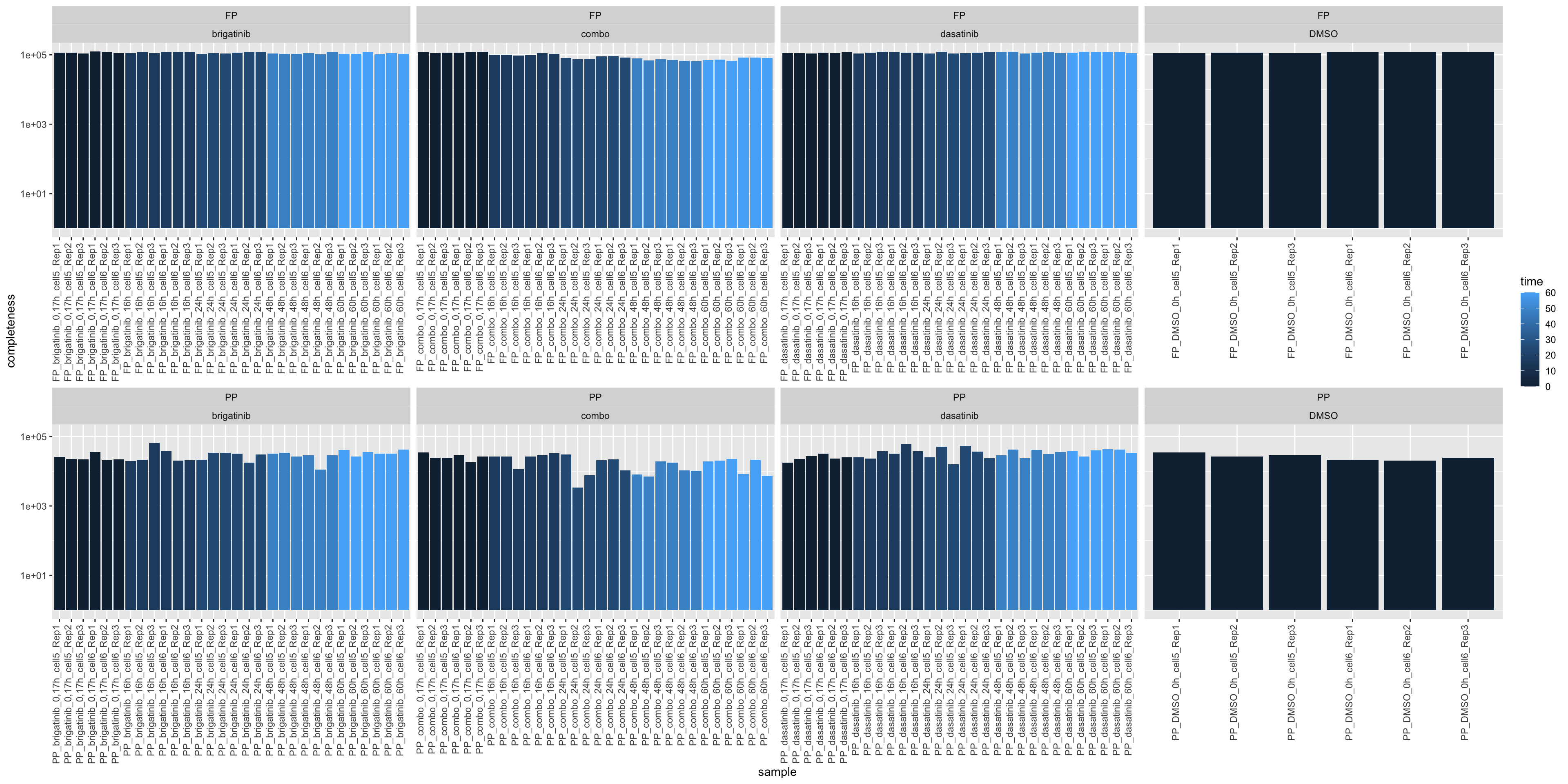
Total intensity
ggplot(sumTab, aes(x=sample, y=total, fill = time)) +
    geom_bar(stat = "identity") +
    ylab("completeness") +
    theme(axis.text.x = element_text(angle = 90, hjust = 1, vjust=0)) +
    facet_wrap(~sampleType+drug, scale = "free_x", ncol=4) +
    scale_y_log10()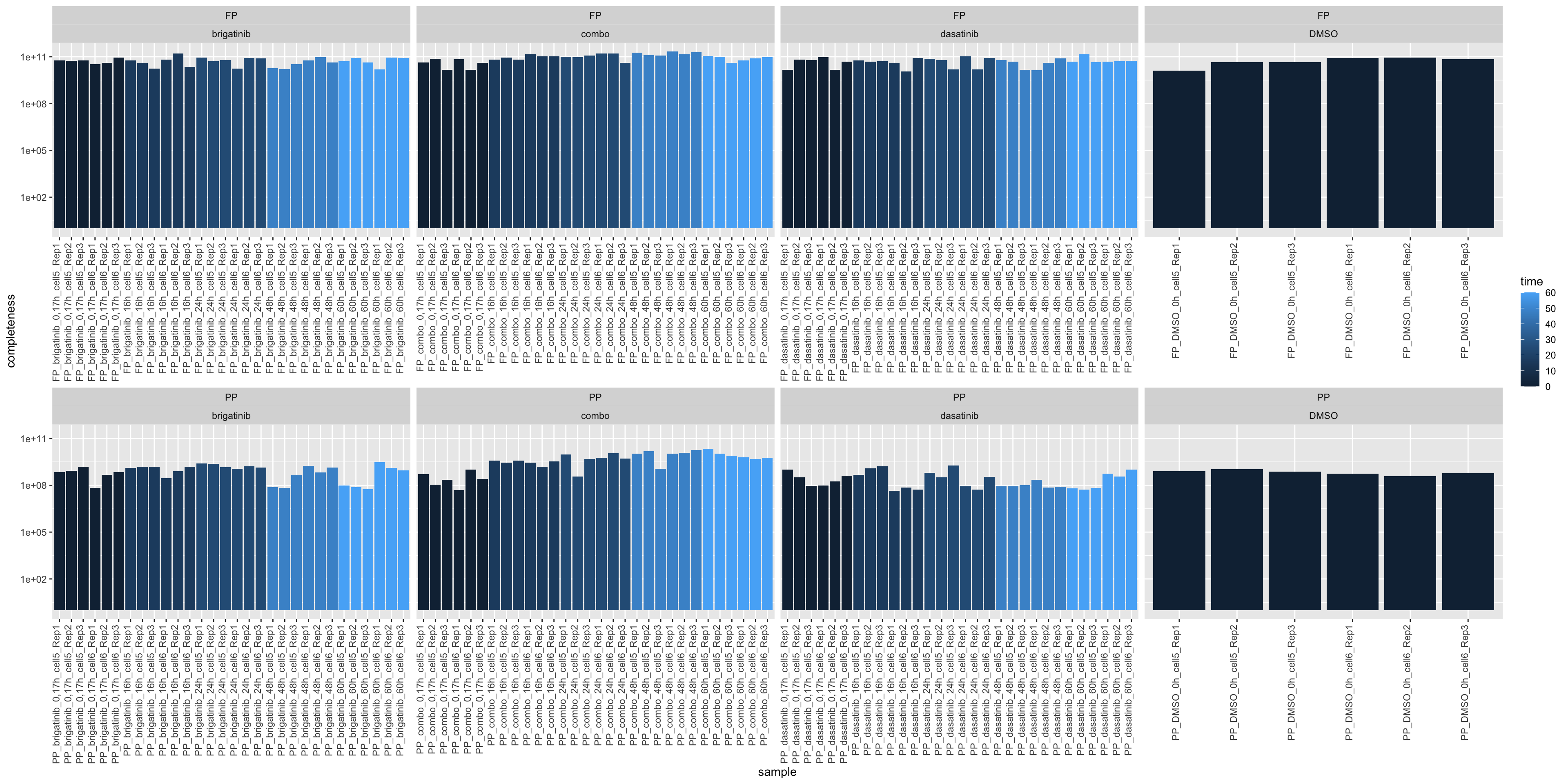
Median Intensity
ggplot(sumTab, aes(x=sample, y=medVal, fill = time)) +
    geom_bar(stat = "identity") +
    ylab("completeness") +
    theme(axis.text.x = element_text(angle = 90, hjust = 1, vjust=0)) +
    facet_wrap(~sampleType+drug, scale = "free_x", ncol=4) +
    scale_y_log10()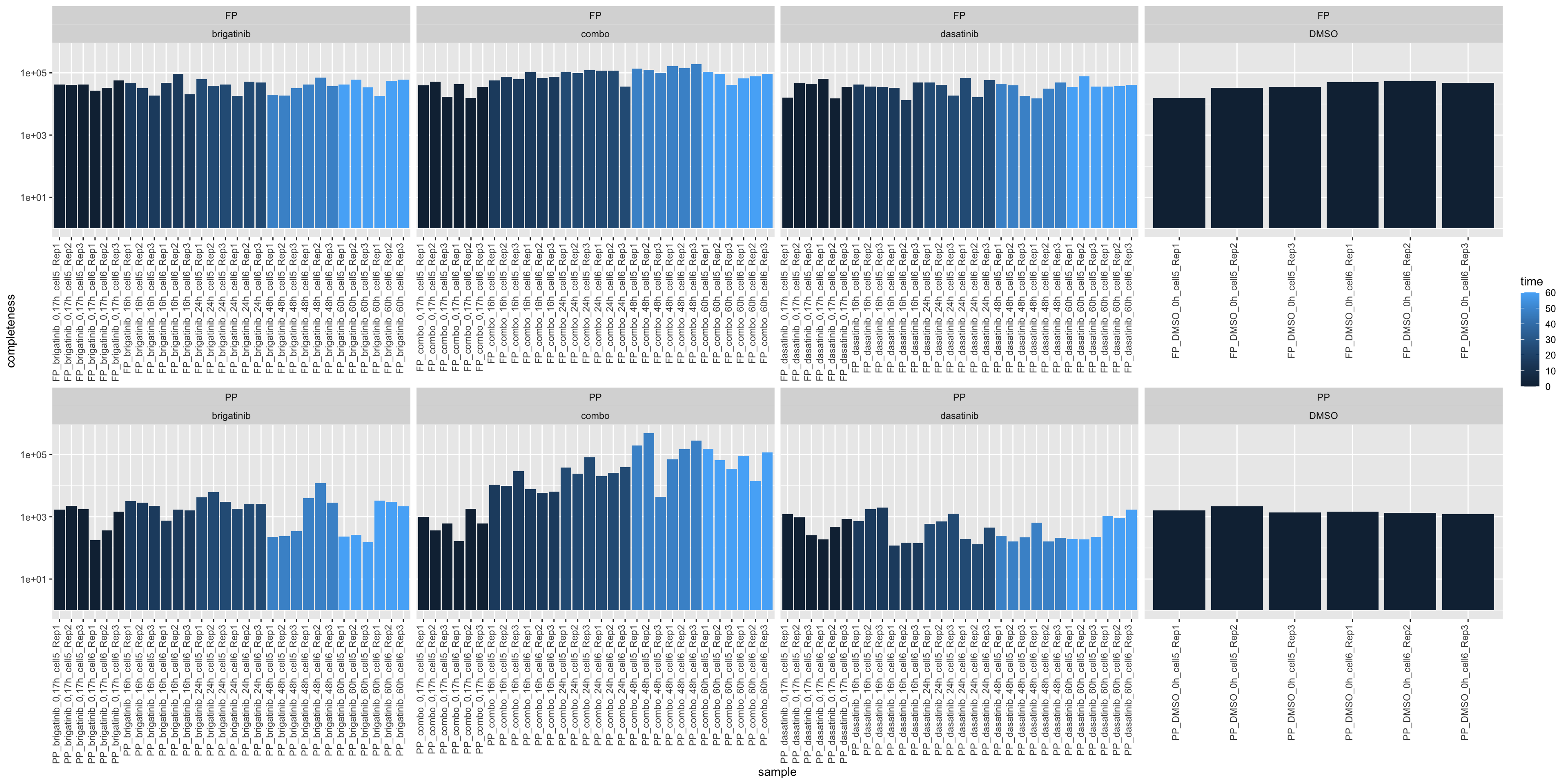
Intensity distribution
FP samples
ggplot(filter(expTab, sampleType == "FP"), aes(y=log2(value), x=sample)) +
  geom_boxplot(aes(fill = time)) +
  facet_wrap(~drug, scale="free_x") +
theme(axis.text.x = element_text(angle = 90, hjust = 1, vjust = 0.5)) 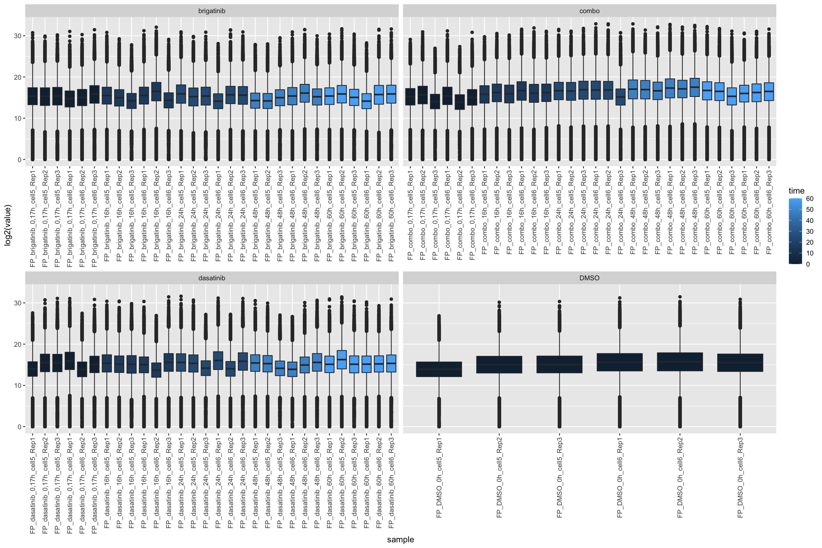
PP samples
ggplot(filter(expTab, sampleType == "PP"), aes(y=log2(value), x=sample)) +
  geom_boxplot(aes(fill = time)) +
  facet_wrap(~drug, scale="free_x") +
theme(axis.text.x = element_text(angle = 90, hjust = 1, vjust = 0.5)) 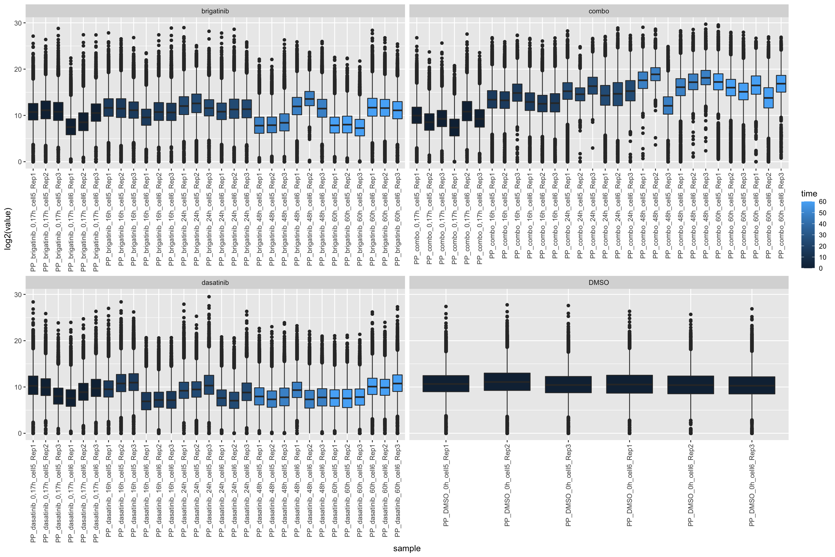
Precurse median table
preMedTab <- group_by(expTab, sample) %>%
  summarise(preMed = median(value)) %>%
  mutate(samplePre = sample) %>%
  mutate(sample = str_replace(sample, ",",".")) %>%
  separate(sample, into = c("a","b","c","d","e"),"_") %>%
  mutate(sample = paste0(a, "_", d, "_", b, "_", c,"_", e)) %>%
  select(sample, samplePre, preMed) %>%
  mutate(logPreMed = log2(preMed),
         scaleFactor = logPreMed/median(logPreMed))
ggplot(preMedTab, aes(x=sample, y=logPreMed)) +
geom_bar(stat = "identity")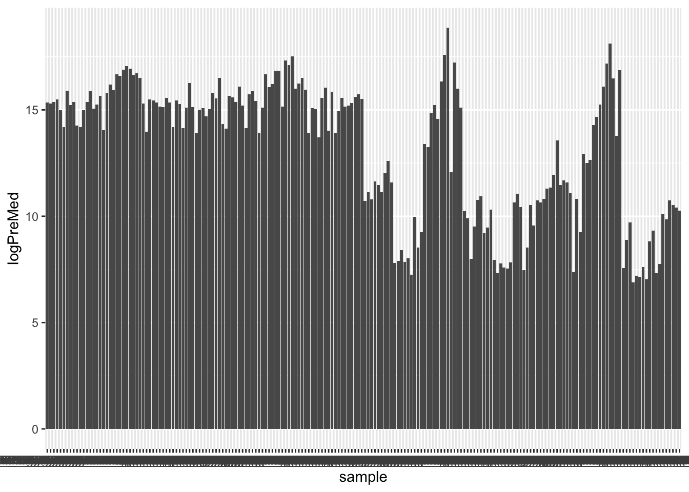
Correlation with median values of protein expression
ppe <- maeData[["Proteome"]]
colData(ppe) <- colData(maeData)

ppeTab <- tibble(sample = paste0(ppe$sampleType,"_",ppe$sample),
                 drug = ppe$drug,
                 med = colMedians(log2(assay(ppe)),na.rm = TRUE),
                 sampleType = ppe$sampleType) %>%
  left_join(preMedTab)
Joining, by = "sample"ggplot(ppeTab, aes(x=med,y=logPreMed)) +
geom_point(aes(col = drug)) +
facet_wrap(~sampleType)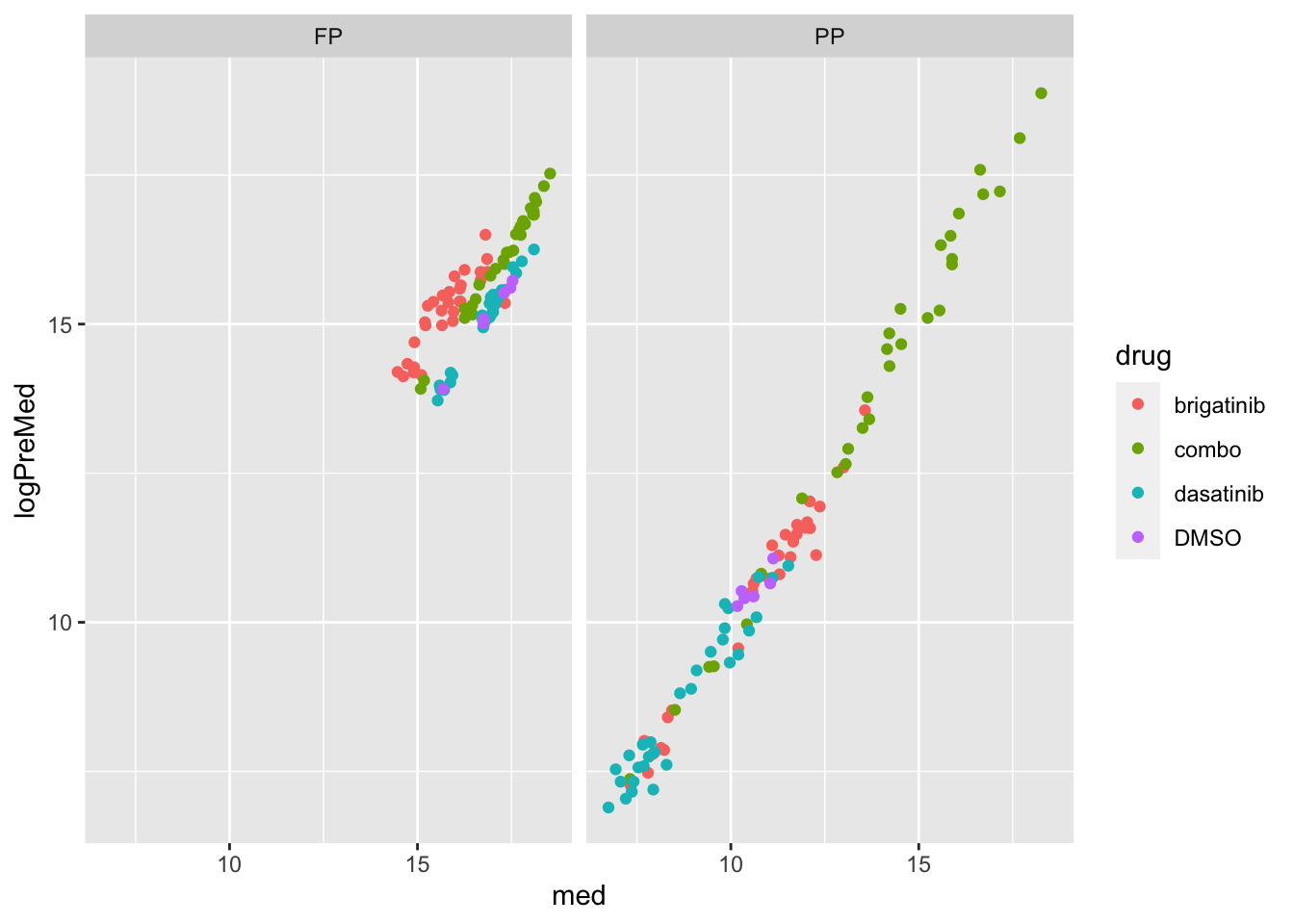
Correlation with median values of phospho expression
ppe <- maeData[["Phosphoproteome"]]
colData(ppe) <- colData(maeData)

ppeTab <- tibble(sample = paste0(ppe$sampleType,"_",ppe$sample),
                 drug = ppe$drug,
                 med = colMedians(log2(assay(ppe)),na.rm = TRUE),
                 sampleType = ppe$sampleType) %>%
  left_join(preMedTab)
Joining, by = "sample"ggplot(ppeTab, aes(x=med,y=logPreMed)) +
geom_point(aes(col = drug)) +
facet_wrap(~sampleType)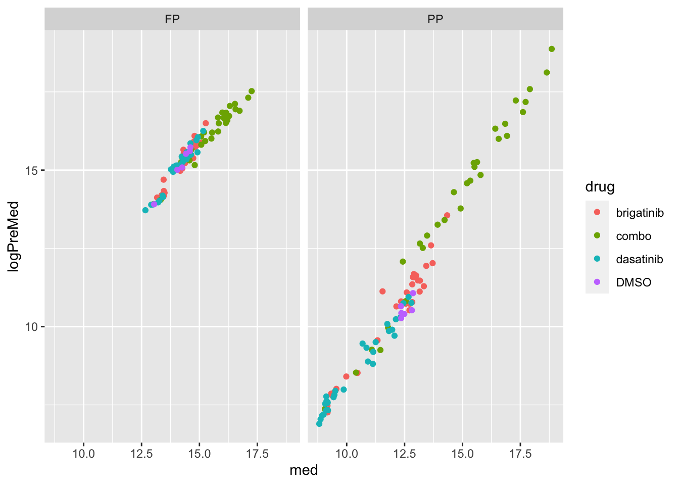 ## Scale using percursur factor
expTab <- mutate(expTab, scaleFactor = preMedTab[match(sample, preMedTab$samplePre),]$scaleFactor) %>%
  mutate(normVal = log2(value)/scaleFactor)
FP samples
ggplot(filter(expTab, sampleType == "FP"), aes(y=normVal, x=sample)) +
  geom_boxplot(aes(fill = time)) +
  facet_wrap(~drug, scale="free_x") +
theme(axis.text.x = element_text(angle = 90, hjust = 1, vjust = 0.5)) 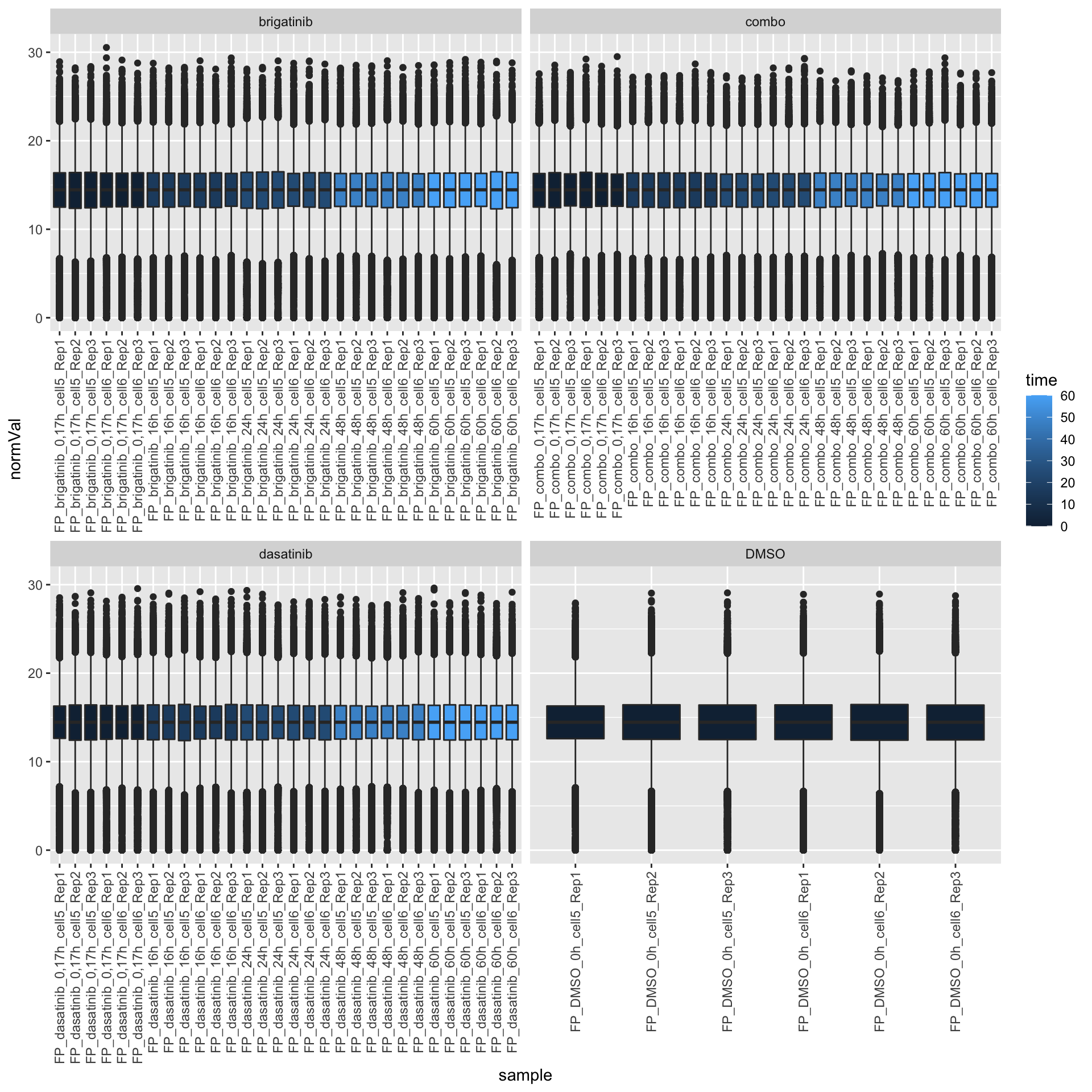
PP samples
ggplot(filter(expTab, sampleType == "PP"), aes(y=normVal, x=sample)) +
  geom_boxplot(aes(fill = time)) +
  facet_wrap(~drug, scale="free_x") +
theme(axis.text.x = element_text(angle = 90, hjust = 1, vjust = 0.5)) 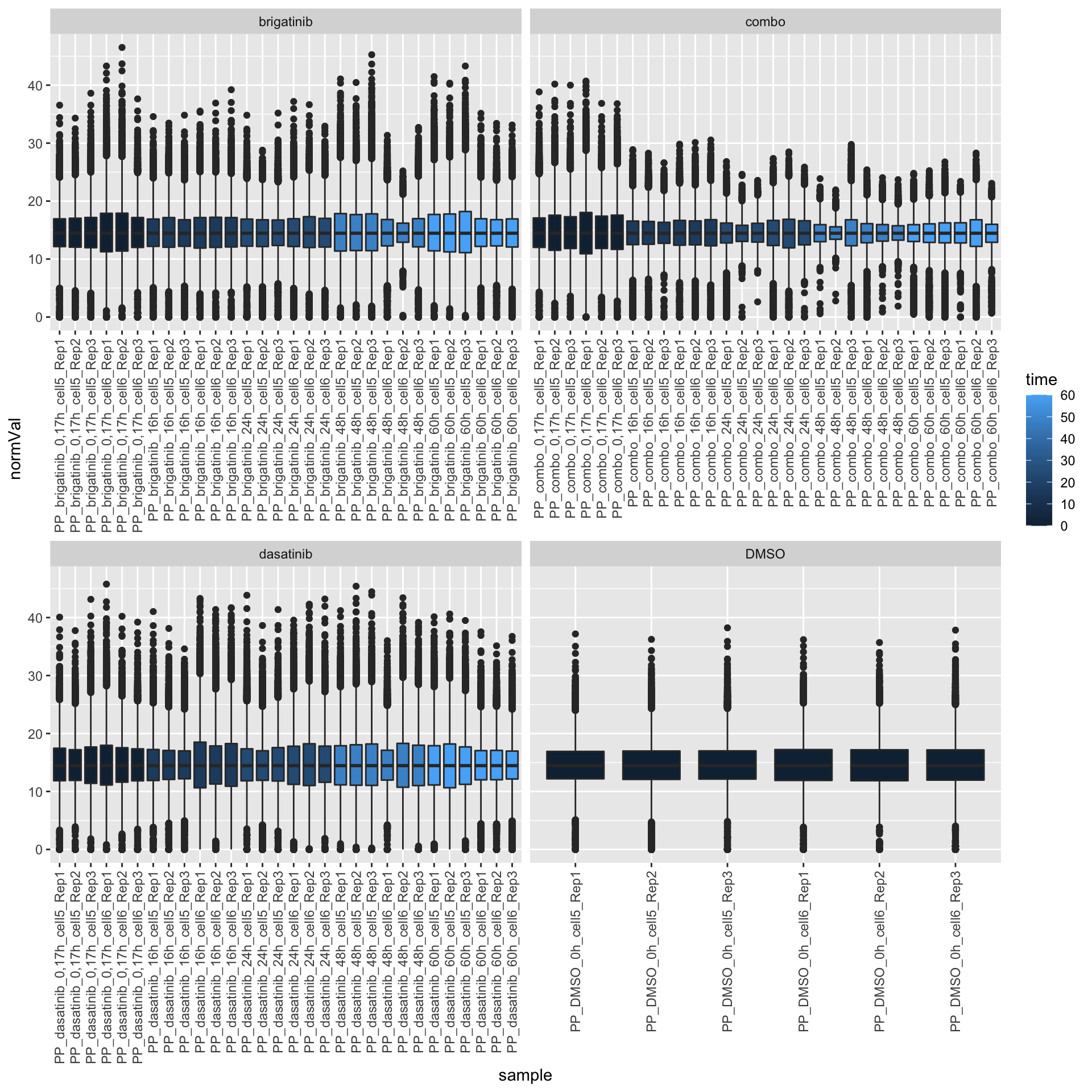
Save scale factor table
scaleFactorTab <- preMedTab %>% select(sample, scaleFactor)
save(scaleFactorTab, file = "../output/scaleFactorTab.RData")
Calculate Phosphorylation ratio or regress protein expression
phosData <- maeData[,maeData$sampleType=="PP"][["Phosphoproteome"]]
protData <- maeData[,maeData$sampleType == "FP"][["Proteome"]]
Completeness of the proteome data
colData(protData) <- colData(maeData[,maeData$sampleType == "FP"])
countMat <- assay(protData)
plotTab <- tibble(sample = protData$sample,
                  perNA = colSums(is.na(countMat))/nrow(countMat),
                  time = protData$time,
                  drug = protData$drug)

ggplot(plotTab, aes(x=sample, y=1-perNA)) +
    geom_bar(stat = "identity", aes(fill = time)) +
    ylab("completeness") +
    facet_wrap(~drug, scales = "free_x") +
theme(axis.text.x = element_text(angle = 90, hjust = 1, vjust=0.5)) 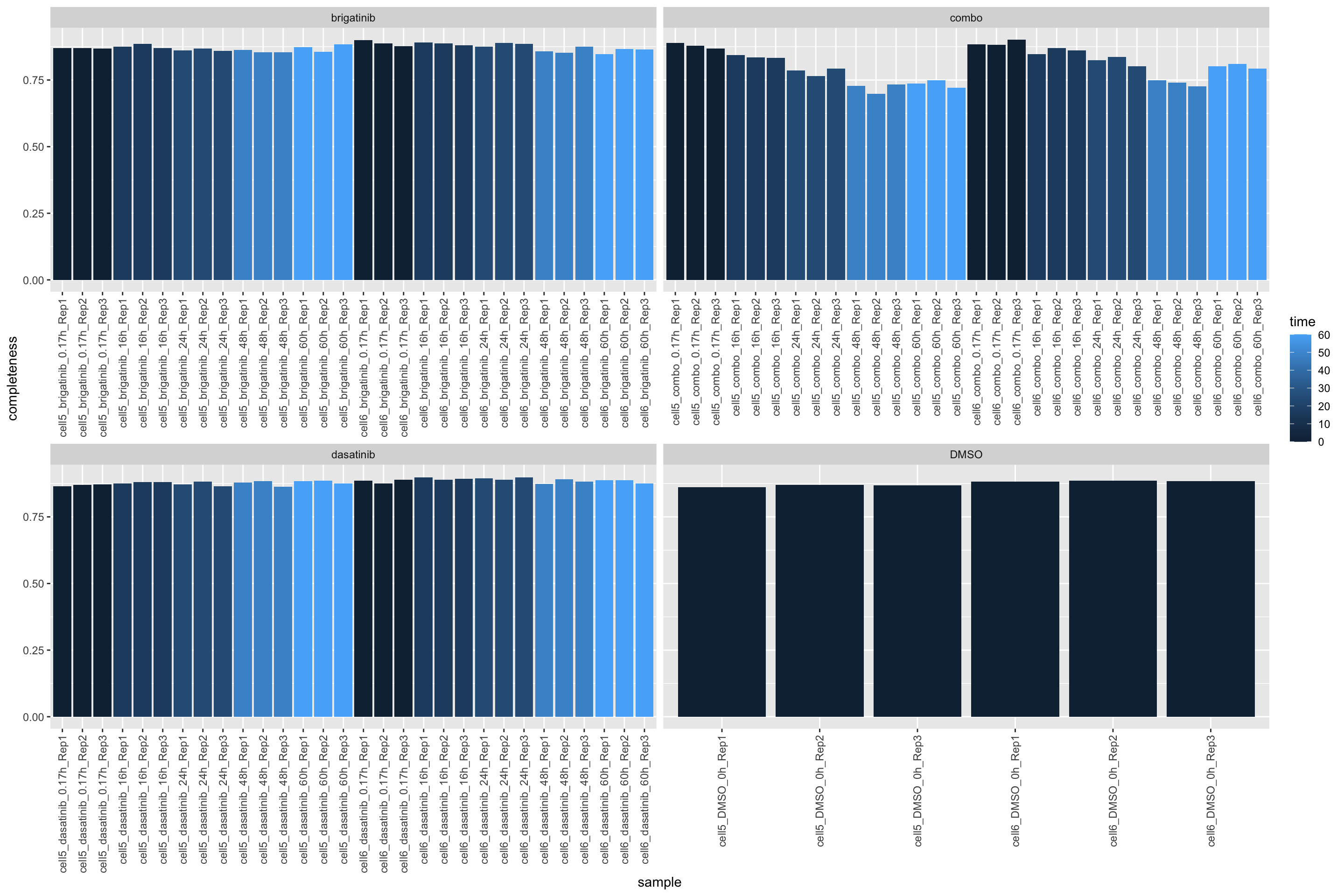
Regression
Phospho data with at least three non-NA value
phosData <- phosData[rowSums(!is.na(assay(phosData))) >= 6,]library(robustbase)
regTab <- lapply(seq(nrow(phosData)), function(i) {
#print(i)
phosVal <- log2(assay(phosData)[i,])
uniID <- rowData(phosData)[i,]$UniprotID
protVal <- log2(assay(protData)[match(uniID, rowData(protData)$UniprotID),])
testTab <- tibble(id = colnames(phosData),
y = phosVal, x = protVal) %>%
filter(!is.na(x), !is.na(y))
if (nrow(testTab) < 6) {
return(NULL)
} else {
if (all(testTab$y == testTab$x)) {
resVal <- residuals(lm(y~x,testTab)) + mean(testTab$y)
} else {
resVal <- residuals(lmrob(y~x,testTab)) + median(testTab$y)
}
r <- cor(testTab$x, testTab$y, use = "pairwise.complete.obs")
return(tibble(smp = testTab$id, residual = resVal, id = rownames(phosData)[i], r=r, diff = testTab$y - testTab$x))
}
}) %>% bind_rows()
corTab <- distinct(regTab, id, r)
regTab$r <- NULL
Warning: The above code chunk cached its results, but
it won’t be re-run if previous chunks it depends on are updated. If you
need to use caching, it is highly recommended to also set
knitr::opts_chunk$set(autodep = TRUE) at the top of the
file (in a chunk that is not cached). Alternatively, you can customize
the option dependson for each individual chunk that is
cached. Using either autodep or dependson will
remove this warning. See the
knitr cache options for more details.
Correlation between protein expression and phospho expression
hist(corTab$r)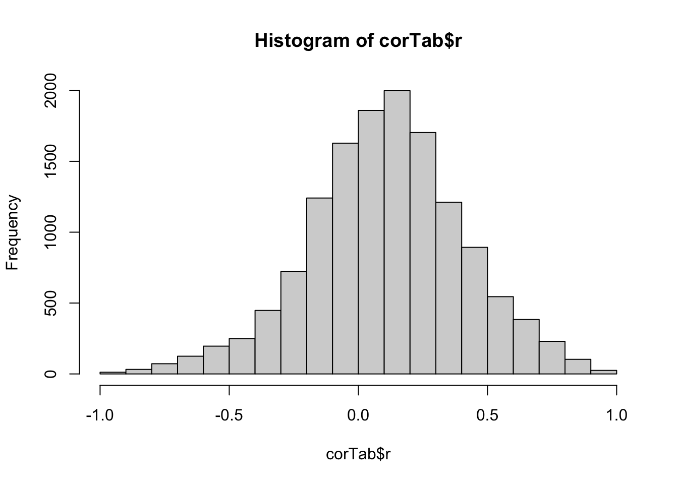
Residue versus ratio
ggplot(regTab, aes(x=residual, y=diff)) +
  geom_hex()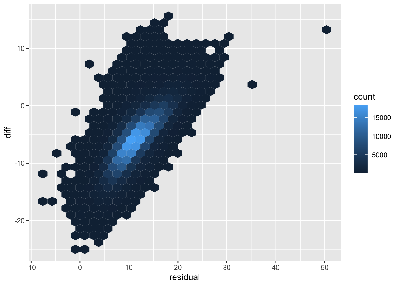
regMat <- select(regTab, id, smp, residual) %>%
  pivot_wider(names_from = smp, values_from = residual) %>%
    column_to_rownames("id") %>% as.matrix()
phosDataReg <- phosData[rownames(regMat), colnames(regMat)]
assay(phosDataReg) <- regMat

diffMat <- select(regTab, id, smp, diff) %>%
  pivot_wider(names_from = smp, values_from = diff) %>%
    column_to_rownames("id") %>% as.matrix()
phosDataRatio <- phosData[rownames(diffMat), colnames(diffMat)]
assay(phosDataRatio) <- diffMat

maeNew <- MultiAssayExperiment::MultiAssayExperiment(experiments = list(
    Proteome = maeData[["Proteome"]],
    Phosphoproteome = maeData[["Phosphoproteome"]],
    PhosReg = phosDataReg,
    PhosRatio = phosDataRatio),
    colData = colData(maeData))
Generate expression matrix
outList <- list()
colAnno <- colData(maeData) %>% as_tibble(rownames = "sample")
Protein level
fpe <- maeData[["Proteome"]]
colData(fpe) <- colData(maeData)
fpe <- fpe[!rowData(fpe)$Gene %in% c("",NA)]
FP sample
outTab <- log2(assay(fpe[,fpe$sampleType == "FP"]))
outTab <- outTab[rowSums(!is.na(outTab))>0, ]
colnames(outTab) <- str_remove(colnames(outTab),"X.[0-9]+..FP_")
outTab <- as_tibble(outTab, rownames = "id") %>%
    mutate(UniprotID = rowData(fpe)[id,]$UniprotID, .before=1) %>%
    mutate(Gene = rowData(fpe)[id,]$Gene, .before=1) %>%
    select(-id)
outList[["Proteome_FP"]] <- outTab
PP sample
outTab <- log2(assay(fpe[,fpe$sampleType == "PP"]))
outTab <- outTab[rowSums(!is.na(outTab))>0, ]
colnames(outTab) <- str_remove(colnames(outTab),"X.[0-9]+..PP_")
outTab <- as_tibble(outTab, rownames = "id") %>%
    mutate(UniprotID = rowData(fpe)[id,]$UniprotID, .before=1) %>%
    mutate(Gene = rowData(fpe)[id,]$Gene, .before=1) %>%
    select(-id)
outList[["Proteome_PP"]] <- outTab
Phosphoproteom level
ppe <- maeData[["Phosphoproteome"]]
colData(ppe) <- colData(maeData)
ppe <- ppe[!rowData(ppe)$Gene %in% c("",NA)]
PP sample
outTab <- log2(assay(ppe[, ppe$sampleType == "PP"]))
outTab <- outTab[rowSums(!is.na(outTab))>0, ]
colnames(outTab) <- str_remove(colnames(outTab),"X.[0-9]+..PP_")
outTab <- as_tibble(outTab, rownames = "id") %>%
    mutate(UniprotID = rowData(ppe)[id,]$UniprotID, .before=1) %>%
    mutate(Site = paste0(rowData(ppe)[id,]$Residue, rowData(ppe)[id,]$Position),.before=1) %>%
    mutate(Gene = rowData(ppe)[id,]$Gene, .before=1) %>%
    select(-id)
outList[["Phosphoproteome_PP"]] <- outTab
FP sample
outTab <- log2(assay(ppe[, ppe$sampleType == "FP"]))
outTab <- outTab[rowSums(!is.na(outTab))>0, ]
colnames(outTab) <- str_remove(colnames(outTab),"X.[0-9]+..FP_")
outTab <- as_tibble(outTab, rownames = "id") %>%
    mutate(UniprotID = rowData(ppe)[id,]$UniprotID, .before=1) %>%
    mutate(Site = paste0(rowData(ppe)[id,]$Residue, rowData(ppe)[id,]$Position),.before=1) %>%
    mutate(Gene = rowData(ppe)[id,]$Gene, .before=1) %>%
    select(-id)
outList[["Phosphoproteome_FP"]] <- outTab
Phospho data with proteomic level regressed out
outTab <- assay(phosDataReg)
outTab <- outTab[rowSums(!is.na(outTab))>0, ]
colnames(outTab) <- str_remove(colnames(outTab),"X.[0-9]+..PP_")
outTab <- as_tibble(outTab, rownames = "id") %>%
    mutate(UniprotID = rowData(phosDataReg)[id,]$UniprotID, .before=1) %>%
    mutate(Site = paste0(rowData(phosDataReg)[id,]$Residue, rowData(phosDataReg)[id,]$Position),.before=1) %>%
    mutate(Gene = rowData(phosDataReg)[id,]$Gene, .before=1) %>%
    select(-id)
outList[["Phosphoproteome_regress"]] <- outTab
Phospho ratio
outTab <- assay(phosDataRatio)
outTab <- outTab[rowSums(!is.na(outTab))>0, ]
colnames(outTab) <- str_remove(colnames(outTab),"X.[0-9]+..PP_")
outTab <- as_tibble(outTab, rownames = "id") %>%
    mutate(UniprotID = rowData(phosDataRatio)[id,]$UniprotID, .before=1) %>%
    mutate(Site = paste0(rowData(phosDataRatio)[id,]$Residue, rowData(phosDataRatio)[id,]$Position),.before=1) %>%
    mutate(Gene = rowData(phosDataRatio)[id,]$Gene, .before=1) %>%
    select(-id)
outList[["Phosphoproteome_ratio"]] <- outTabSave objects
maeData <- maeNew
save(maeData, file = "../output/processedData.RData")
sessionInfo()R version 4.2.0 (2022-04-22)
Platform: x86_64-apple-darwin17.0 (64-bit)
Running under: macOS Big Sur/Monterey 10.16
Matrix products: default
BLAS: /Library/Frameworks/R.framework/Versions/4.2/Resources/lib/libRblas.0.dylib
LAPACK: /Library/Frameworks/R.framework/Versions/4.2/Resources/lib/libRlapack.dylib
locale:
[1] en_US.UTF-8/en_US.UTF-8/en_US.UTF-8/C/en_US.UTF-8/en_US.UTF-8
attached base packages:
[1] stats4 stats graphics grDevices utils datasets methods
[8] base
other attached packages:
[1] robustbase_0.95-0 forcats_0.5.1
[3] stringr_1.4.1 dplyr_1.0.9
[5] purrr_0.3.4 readr_2.1.2
[7] tidyr_1.2.0 tibble_3.1.8
[9] ggplot2_3.3.6 tidyverse_1.3.2
[11] SummarizedExperiment_1.26.1 Biobase_2.56.0
[13] GenomicRanges_1.48.0 GenomeInfoDb_1.32.2
[15] IRanges_2.30.0 S4Vectors_0.34.0
[17] BiocGenerics_0.42.0 MatrixGenerics_1.8.1
[19] matrixStats_0.62.0 DEP_1.18.0
[21] PhosR_1.6.0 SmartPhos_0.1.0
loaded via a namespace (and not attached):
[1] utf8_1.2.2 shinydashboard_0.7.2
[3] gmm_1.6-6 tidyselect_1.1.2
[5] htmlwidgets_1.5.4 grid_4.2.0
[7] BiocParallel_1.30.3 norm_1.0-10.0
[9] munsell_0.5.0 codetools_0.2-18
[11] preprocessCore_1.58.0 DT_0.23
[13] withr_2.5.0 colorspace_2.0-3
[15] highr_0.9 knitr_1.39
[17] rstudioapi_0.13 ggsignif_0.6.3
[19] mzID_1.34.0 labeling_0.4.2
[21] git2r_0.30.1 GenomeInfoDbData_1.2.8
[23] bit64_4.0.5 farver_2.1.1
[25] pheatmap_1.0.12 rprojroot_2.0.3
[27] coda_0.19-4 vctrs_0.4.1
[29] generics_0.1.3 xfun_0.31
[31] R6_2.5.1 doParallel_1.0.17
[33] clue_0.3-61 MsCoreUtils_1.8.0
[35] bitops_1.0-7 cachem_1.0.6
[37] reshape_0.8.9 DelayedArray_0.22.0
[39] assertthat_0.2.1 vroom_1.5.7
[41] promises_1.2.0.1 scales_1.2.0
[43] googlesheets4_1.0.0 gtable_0.3.0
[45] Cairo_1.6-0 affy_1.74.0
[47] sandwich_3.0-2 workflowr_1.7.0
[49] rlang_1.0.6 mzR_2.30.0
[51] splines_4.2.0 GlobalOptions_0.1.2
[53] rstatix_0.7.0 gargle_1.2.0
[55] impute_1.70.0 hexbin_1.28.2
[57] broom_1.0.0 BiocManager_1.30.18
[59] yaml_2.3.5 reshape2_1.4.4
[61] abind_1.4-5 modelr_0.1.8
[63] backports_1.4.1 httpuv_1.6.6
[65] tools_4.2.0 statnet.common_4.6.0
[67] affyio_1.66.0 ellipsis_0.3.2
[69] jquerylib_0.1.4 RColorBrewer_1.1-3
[71] ggdendro_0.1.23 proxy_0.4-27
[73] MSnbase_2.22.0 MultiAssayExperiment_1.22.0
[75] Rcpp_1.0.9 plyr_1.8.7
[77] zlibbioc_1.42.0 RCurl_1.98-1.7
[79] ggpubr_0.4.0 GetoptLong_1.0.5
[81] viridis_0.6.2 zoo_1.8-10
[83] haven_2.5.0 cluster_2.1.3
[85] fs_1.5.2 magrittr_2.0.3
[87] data.table_1.14.2 circlize_0.4.15
[89] reprex_2.0.1 googledrive_2.0.0
[91] pcaMethods_1.88.0 mvtnorm_1.1-3
[93] ProtGenerics_1.28.0 hms_1.1.1
[95] mime_0.12 evaluate_0.15
[97] xtable_1.8-4 XML_3.99-0.10
[99] readxl_1.4.0 gridExtra_2.3
[101] shape_1.4.6 compiler_4.2.0
[103] writexl_1.4.0 ncdf4_1.19
[105] crayon_1.5.2 htmltools_0.5.3
[107] mgcv_1.8-40 later_1.3.0
[109] tzdb_0.3.0 lubridate_1.8.0
[111] DBI_1.1.3 dbplyr_2.2.1
[113] ComplexHeatmap_2.12.0 MASS_7.3-58
[115] tmvtnorm_1.5 Matrix_1.4-1
[117] car_3.1-0 cli_3.4.1
[119] vsn_3.64.0 imputeLCMD_2.1
[121] parallel_4.2.0 igraph_1.3.4
[123] pkgconfig_2.0.3 MALDIquant_1.21
[125] xml2_1.3.3 foreach_1.5.2
[127] bslib_0.4.1 XVector_0.36.0
[129] ruv_0.9.7.1 rvest_1.0.2
[131] digest_0.6.30 rmarkdown_2.14
[133] cellranger_1.1.0 dendextend_1.16.0
[135] shiny_1.7.3 rjson_0.2.21
[137] nlme_3.1-158 lifecycle_1.0.3
[139] jsonlite_1.8.3 carData_3.0-5
[141] network_1.17.2 viridisLite_0.4.0
[143] limma_3.52.2 fansi_1.0.3
[145] pillar_1.8.0 lattice_0.20-45
[147] GGally_2.1.2 DEoptimR_1.0-11
[149] fastmap_1.1.0 httr_1.4.3
[151] glue_1.6.2 png_0.1-7
[153] iterators_1.0.14 bit_4.0.4
[155] class_7.3-20 stringi_1.7.8
[157] sass_0.4.2 e1071_1.7-11