Analysis of gene dosage effect related to trisomy19
Junyan Lu
2020-02-27
Last updated: 2020-05-29
Checks: 6 1
Knit directory: Proteomics/analysis/
This reproducible R Markdown analysis was created with workflowr (version 1.6.0). The Checks tab describes the reproducibility checks that were applied when the results were created. The Past versions tab lists the development history.
The R Markdown is untracked by Git. To know which version of the R Markdown file created these results, you’ll want to first commit it to the Git repo. If you’re still working on the analysis, you can ignore this warning. When you’re finished, you can run wflow_publish to commit the R Markdown file and build the HTML.
Great job! The global environment was empty. Objects defined in the global environment can affect the analysis in your R Markdown file in unknown ways. For reproduciblity it’s best to always run the code in an empty environment.
The command set.seed(20200227) was run prior to running the code in the R Markdown file. Setting a seed ensures that any results that rely on randomness, e.g. subsampling or permutations, are reproducible.
Great job! Recording the operating system, R version, and package versions is critical for reproducibility.
Nice! There were no cached chunks for this analysis, so you can be confident that you successfully produced the results during this run.
Great job! Using relative paths to the files within your workflowr project makes it easier to run your code on other machines.
Great! You are using Git for version control. Tracking code development and connecting the code version to the results is critical for reproducibility. The version displayed above was the version of the Git repository at the time these results were generated.
Note that you need to be careful to ensure that all relevant files for the analysis have been committed to Git prior to generating the results (you can use wflow_publish or wflow_git_commit). workflowr only checks the R Markdown file, but you know if there are other scripts or data files that it depends on. Below is the status of the Git repository when the results were generated:
Ignored files:
    Ignored:    .DS_Store
    Ignored:    .Rhistory
    Ignored:    .Rproj.user/
    Ignored:    analysis/.DS_Store
    Ignored:    analysis/.Rhistory
    Ignored:    analysis/complexAnalysis_IGHV_cache/
    Ignored:    analysis/complexAnalysis_trisomy12_alteredPQR_cache/
    Ignored:    analysis/complexAnalysis_trisomy12_cache/
    Ignored:    analysis/correlateCLLPD_cache/
    Ignored:    code/.Rhistory
    Ignored:    data/.DS_Store
    Ignored:    output/.DS_Store

Untracked files:
    Untracked:  analysis/CNVanalysis_trisomy12.Rmd
    Untracked:  analysis/CNVanalysis_trisomy19.Rmd
    Untracked:  analysis/analysisSplicing.Rmd
    Untracked:  analysis/analysisTrisomy19.Rmd
    Untracked:  analysis/annotateCNV.Rmd
    Untracked:  analysis/complexAnalysis_IGHV.Rmd
    Untracked:  analysis/complexAnalysis_trisomy12.Rmd
    Untracked:  analysis/correlateGenomic_PC12adjusted.Rmd
    Untracked:  analysis/correlateGenomic_noBlock.Rmd
    Untracked:  analysis/correlateGenomic_noBlock_MCLL.Rmd
    Untracked:  analysis/correlateGenomic_noBlock_UCLL.Rmd
    Untracked:  analysis/default.css
    Untracked:  analysis/del11q.pdf
    Untracked:  analysis/del11q_norm.pdf
    Untracked:  analysis/peptideValidate.Rmd
    Untracked:  analysis/plotCNV_del11q.pdf
    Untracked:  analysis/plotExpressionCNV.Rmd
    Untracked:  analysis/processPeptides_LUMOS.Rmd
    Untracked:  analysis/style.css
    Untracked:  analysis/trisomy12.pdf
    Untracked:  analysis/trisomy12_AFcor.Rmd
    Untracked:  analysis/trisomy12_norm.pdf
    Untracked:  code/AlteredPQR.R
    Untracked:  code/utils.R
    Untracked:  data/190909_CLL_prot_abund_med_norm.tsv
    Untracked:  data/190909_CLL_prot_abund_no_norm.tsv
    Untracked:  data/20190423_Proteom_submitted_samples_bereinigt.xlsx
    Untracked:  data/20191025_Proteom_submitted_samples_final.xlsx
    Untracked:  data/LUMOS/
    Untracked:  data/LUMOS_peptides/
    Untracked:  data/LUMOS_protAnnotation.csv
    Untracked:  data/LUMOS_protAnnotation_fix.csv
    Untracked:  data/SampleAnnotation_cleaned.xlsx
    Untracked:  data/example_proteomics_data
    Untracked:  data/facTab_IC50atLeast3New.RData
    Untracked:  data/gmts/
    Untracked:  data/mapEnsemble.txt
    Untracked:  data/mapSymbol.txt
    Untracked:  data/proteins_in_complexes
    Untracked:  data/pyprophet_export_aligned.csv
    Untracked:  data/timsTOF_protAnnotation.csv
    Untracked:  output/LUMOS_processed.RData
    Untracked:  output/cnv_plots.zip
    Untracked:  output/cnv_plots/
    Untracked:  output/cnv_plots_norm.zip
    Untracked:  output/dxdCLL.RData
    Untracked:  output/exprCNV.RData
    Untracked:  output/pepCLL_lumos.RData
    Untracked:  output/pepTab_lumos.RData
    Untracked:  output/plotCNV_allChr11_diff.pdf
    Untracked:  output/plotCNV_del11q_sum.pdf
    Untracked:  output/proteomic_LUMOS_20200227.RData
    Untracked:  output/proteomic_LUMOS_20200320.RData
    Untracked:  output/proteomic_LUMOS_20200430.RData
    Untracked:  output/proteomic_timsTOF_20200227.RData
    Untracked:  output/splicingResults.RData
    Untracked:  output/timsTOF_processed.RData
    Untracked:  plotCNV_del11q_diff.pdf

Unstaged changes:
    Modified:   analysis/_site.yml
    Modified:   analysis/analysisSF3B1.Rmd
    Modified:   analysis/compareProteomicsRNAseq.Rmd
    Modified:   analysis/correlateCLLPD.Rmd
    Modified:   analysis/correlateGenomic.Rmd
    Deleted:    analysis/correlateGenomic_removePC.Rmd
    Modified:   analysis/correlateMIR.Rmd
    Modified:   analysis/correlateMethylationCluster.Rmd
    Modified:   analysis/index.Rmd
    Modified:   analysis/predictOutcome.Rmd
    Modified:   analysis/processProteomics_LUMOS.Rmd
    Modified:   analysis/qualityControl_LUMOS.Rmd
Note that any generated files, e.g. HTML, png, CSS, etc., are not included in this status report because it is ok for generated content to have uncommitted changes.
There are no past versions. Publish this analysis with wflow_publish() to start tracking its development.
load("../../var/ddsrna_180717.RData")
load("../../var/patmeta_200522.RData")
load("../../var/proteomic_LUMOS_20200430.RData")
load("../output/exprCNV.RData")
Subset samples to M-CLL with trisomy12
protCLL$trisomy19 <- patMeta[match(colnames(protCLL),patMeta$Patient.ID),]$trisomy19
patTab <- colData(protCLL) %>% data.frame() %>% rownames_to_column("patID") %>%
  filter(IGHV.status %in% "M", trisomy12 %in% 1, !is.na(trisomy19))
dds <- dds[,dds$PatID %in% patTab$patID]
allRnaTab <- filter(allRnaTab, patID %in% patTab$patID)
allProtTab <- filter(allProtTab, patID %in% patTab$patID)
Compare gene dosage effect on RNA and protein level
Gene dosage effect on RNA level
#remove genes never expressed
noExpTab <- group_by(allRnaTab, id) %>% summarise(sumExpr = sum(expr)) %>%
  filter(sumExpr == 0)
#mean variance trend
meanVarTab <- group_by(allRnaTab, id) %>%
summarise(meanVal = mean(expr),varVal = var(expr))
plot(meanVarTab$meanVal, meanVarTab$varVal)
#looks fine for exploratory analysisrnaExprTab <- allRnaTab %>% filter(!id%in% noExpTab$id) %>%
mutate(trisomy19 = patMeta[match(patID, patMeta$Patient.ID),]$trisomy19) %>%
filter(!is.na(trisomy19)) %>% mutate(cnv = ifelse(trisomy19 %in% 1, "trisomy19","wt"))Compare expression levels of Chr19 genes in tri19 and wt samples
Raw counts
meanExprChr19 <- rnaExprTab %>% filter(ChromID %in% "chr19") %>%
group_by(id, symbol, cnv) %>% summarise(meanExpr = mean(expr, na.rm=TRUE)) %>%
ungroup()
ggplot(meanExprChr19, aes(x=meanExpr, fill = cnv)) + geom_histogram(position = "identity", alpha=0.5) 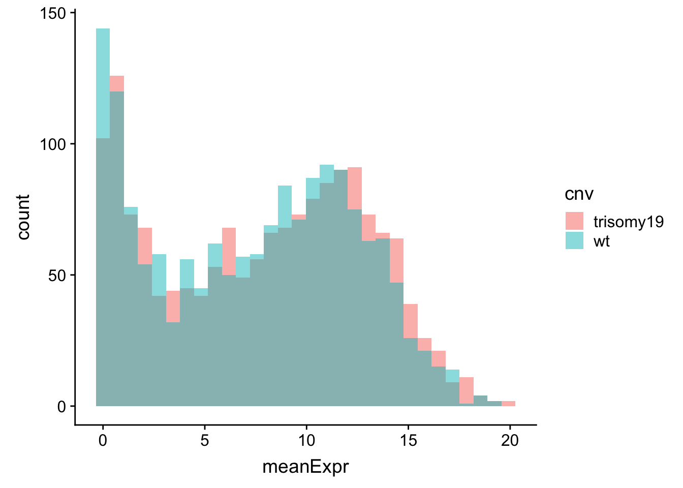 There is no strong different, this is because the baseline expression values among genes are much larger than the relative expression difference between trisomy19 and wt samples.
Expression values centered by mean
meanExprChr19 <- rnaExprTab %>% filter(ChromID %in% "chr19") %>%
group_by(id) %>% mutate(med=mean(expr),sd = sd(expr)) %>% mutate(expr = (expr-med)) %>%
group_by(id, symbol, cnv) %>% summarise(meanExpr = mean(expr, na.rm=TRUE)) %>%
ungroup()
ggplot(meanExprChr19, aes(x=meanExpr, fill = cnv)) + geom_histogram(position = "identity", alpha=0.5) 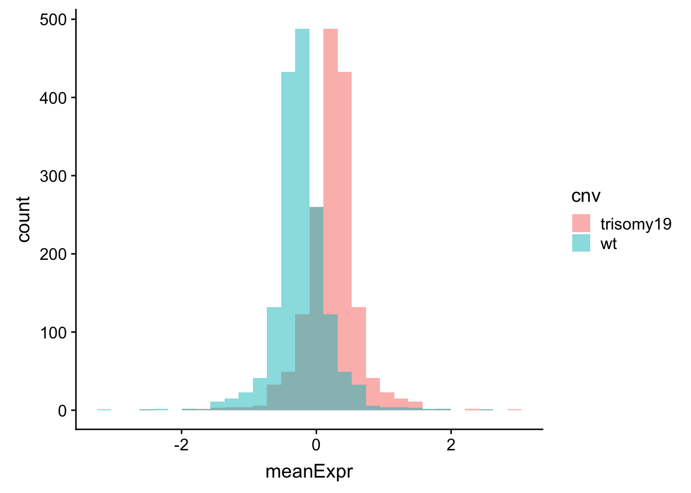 Now the difference is clearly visible.
Mean expression difference between trisomy19 and wt samples for the genes on chr19 and other chromosomes
plotTab <- rnaExprTab %>%
group_by(id, cnv, ChromID) %>% summarise(meanExpr = mean(expr, na.rm=TRUE)) %>%
ungroup() %>%
spread(key = cnv, value = meanExpr) %>%
mutate(diff = trisomy19-wt) %>%
mutate(chr = ifelse(ChromID == "chr19","Chr19","Other"))
ggplot(plotTab, aes(x=diff, fill = chr, y = ..density..)) + geom_histogram(position = "identity", alpha=0.5) +
xlab("Mean expression difference")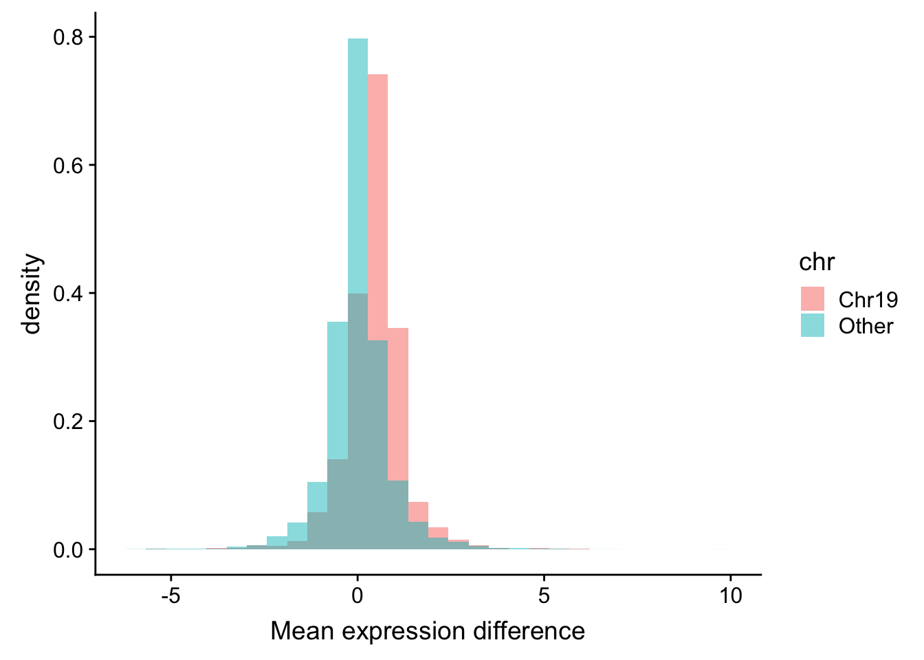 It’s also visible that most genes on chr19 tend to have higher expression in trisomy19 samples. While other genes follow normal distribution centered at 0.
Gene dosage effect on protein level
protExprTab <- allProtTab %>%
  mutate(trisomy19 = patMeta[match(patID, patMeta$Patient.ID),]$trisomy19) %>%
  filter(!is.na(trisomy19)) %>% mutate(cnv = ifelse(trisomy19 %in% 1, "trisomy19","wt"))
Compare expression levels of Chr19 genes in tri19 and wt samples
Raw counts
meanExprChr19 <- protExprTab %>% filter(ChromID %in% "chr19") %>%
group_by(id, symbol, cnv) %>% summarise(meanExpr = mean(expr, na.rm=TRUE)) %>%
ungroup()
ggplot(meanExprChr19, aes(x=meanExpr, fill = cnv)) + geom_histogram(position = "identity", alpha=0.5) 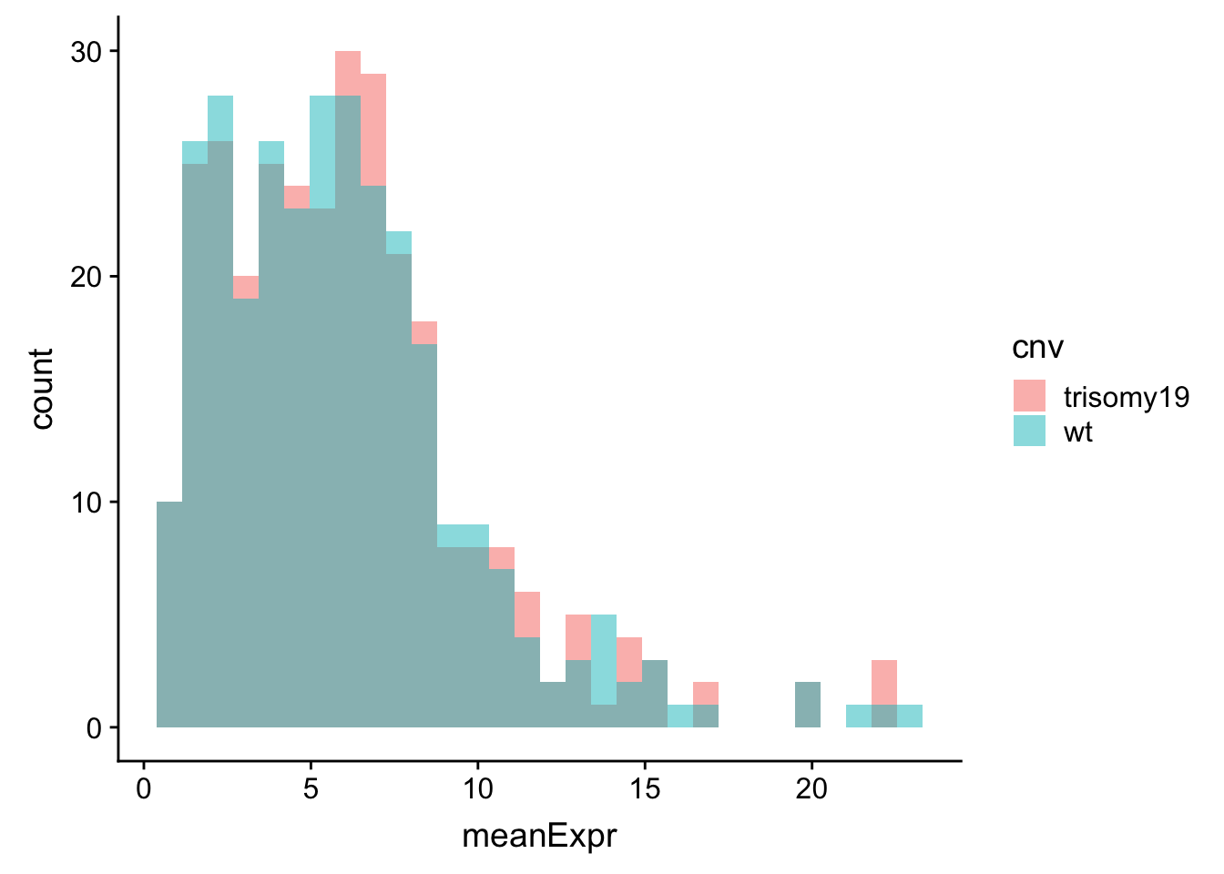 Similar as in the RNA expression, the difference is not very visible when raw count is used.
Expression values centered by mean
meanExprChr19 <- protExprTab %>% filter(ChromID %in% "chr19") %>%
group_by(id) %>% mutate(med=mean(expr),sd = sd(expr)) %>% mutate(expr = (expr-med)) %>%
group_by(id, symbol, cnv) %>% summarise(meanExpr = mean(expr, na.rm=TRUE)) %>%
ungroup()
ggplot(meanExprChr19, aes(x=meanExpr, fill = cnv)) + geom_histogram(position = "identity", alpha=0.5) 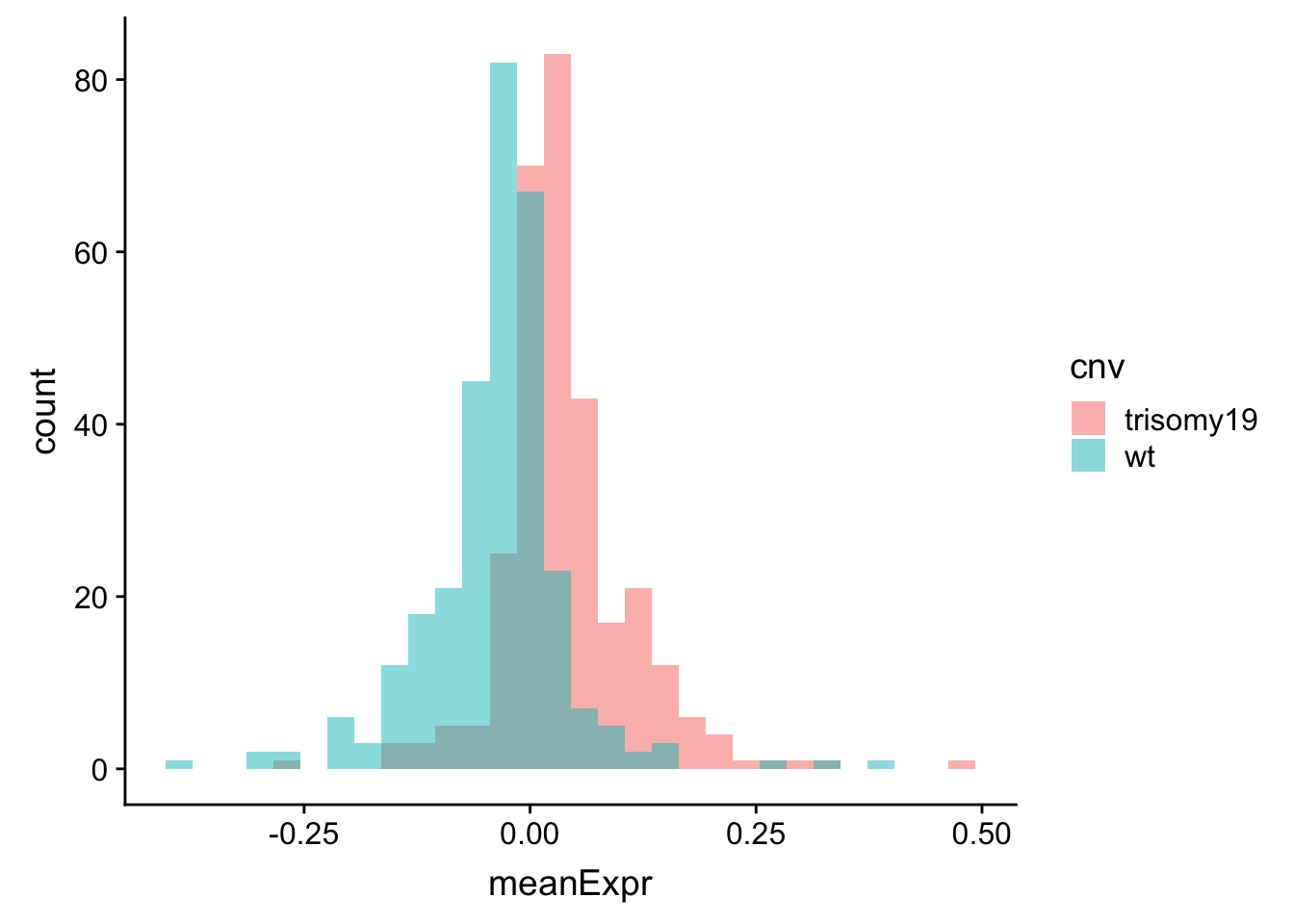 Now difference is clearly visible.
Mean protein expression difference between trisomy19 and wt samples for the genes on chr19 and other chromosomes
plotTab <- protExprTab %>%
group_by(id, cnv, ChromID) %>% summarise(meanExpr = mean(expr, na.rm=TRUE)) %>%
ungroup() %>%
spread(key = cnv, value = meanExpr) %>%
mutate(diff = trisomy19-wt) %>%
mutate(chr = ifelse(ChromID == "chr19","Chr19","Other"))
ggplot(plotTab, aes(x=diff, fill = chr, y = ..density..)) + geom_histogram(position = "identity", alpha=0.5) 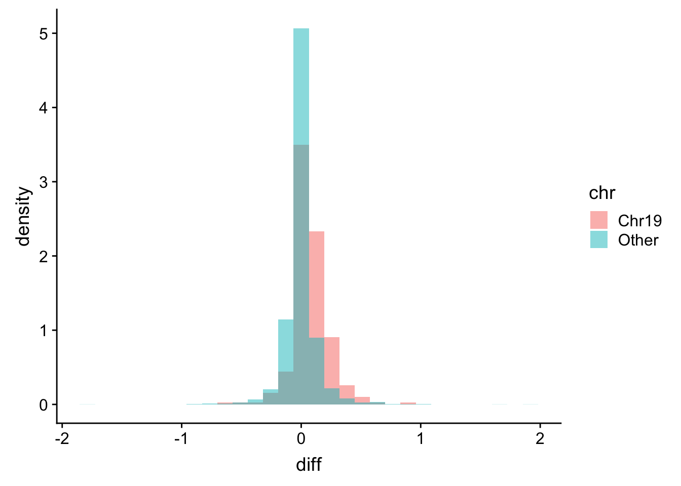 The gene dosage effect is also clearly visible in the proteomic dataset
Compare the gene dosage effect between RNA and protein data
Variance of chr19 gene expression
varRna <- filter(rnaExprTab, ChromID == "chr19") %>%
group_by(id,trisomy19) %>% summarise(sd = sd(expr)) %>%
mutate(set = "rna")
varProt <- filter(protExprTab, ChromID == "chr19") %>%
group_by(id,trisomy19) %>% summarise(sd = sd(expr)) %>%
mutate(set = "protein")
plotTab <- bind_rows(varRna, varProt) %>% ungroup()
ggplot(plotTab, aes(x=sd, fill = set, y = ..density..)) +
geom_histogram(position = "identity", alpha=0.5, bins = 100)+
facet_wrap(~trisomy19) + xlab("Expression variance")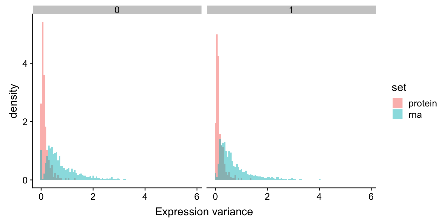 The variance of RNA expression is higher than protein expression, which is an indication of buffering. The trend is the same in samples with or without trisomy19
Expression value (centered by mean)
expRna <- filter(rnaExprTab, ChromID == "chr19") %>%
group_by(id) %>% mutate(meanVal = mean(expr)) %>%
mutate(expr = expr-meanVal) %>%
group_by(id,trisomy19) %>%
summarise(meanExpr = mean(expr)) %>%
mutate(set = "rna")
expProt <- filter(protExprTab, ChromID == "chr19") %>%
group_by(id) %>% mutate(meanVal = mean(expr)) %>%
mutate(expr = expr-meanVal) %>%
group_by(id,trisomy19) %>%
summarise(meanExpr = mean(expr)) %>%
mutate(set = "protein")
plotTab <- bind_rows(expRna, expProt)
ggplot(plotTab, aes(x=meanExpr, fill = set, y = ..density..)) +
geom_histogram(position = "identity", alpha=0.5, bins = 100) +
facet_wrap(~trisomy19) +
xlab("Mean expression")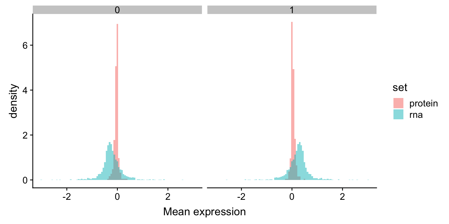 The RNA expression change is larger than protein expression change.
Plot the log fold change of RNA and proteins on chr19 (trisomy19 VS WT)
protDiffTab <- protExprTab %>%
group_by(id, cnv, ChromID) %>% summarise(meanExpr = mean(expr, na.rm=TRUE)) %>%
ungroup() %>%
spread(key = cnv, value = meanExpr) %>%
mutate(diffProt = log(trisomy19/wt)) %>%
mutate(chr = ifelse(ChromID == "chr19","Chr19","Other")) %>%
select(id, diffProt, chr)
rnaDiffTab <- rnaExprTab %>%
group_by(id, cnv, ChromID) %>% summarise(meanExpr = mean(expr, na.rm=TRUE)) %>%
ungroup() %>%
spread(key = cnv, value = meanExpr) %>%
mutate(diffRna = log(trisomy19/wt)) %>% select(id, diffRna)
compareTab <- left_join(protDiffTab, rnaDiffTab, by = "id") %>%
filter(!is.na(diffProt),!is.na(diffRna)) %>%
gather(key = dataset, value=diff,-id,-chr) %>%
mutate(group =paste0(chr,"_",dataset)) %>%
filter(chr == "Chr19")
ggplot(compareTab, aes(x=diff, fill = group, y = ..density..)) +
geom_histogram(position = "identity", alpha=0.5, bins = 100) +
geom_vline(xintercept = 0, color = "blue", linetype ="dashed") +
xlab("Expression different (tri19 - wt)")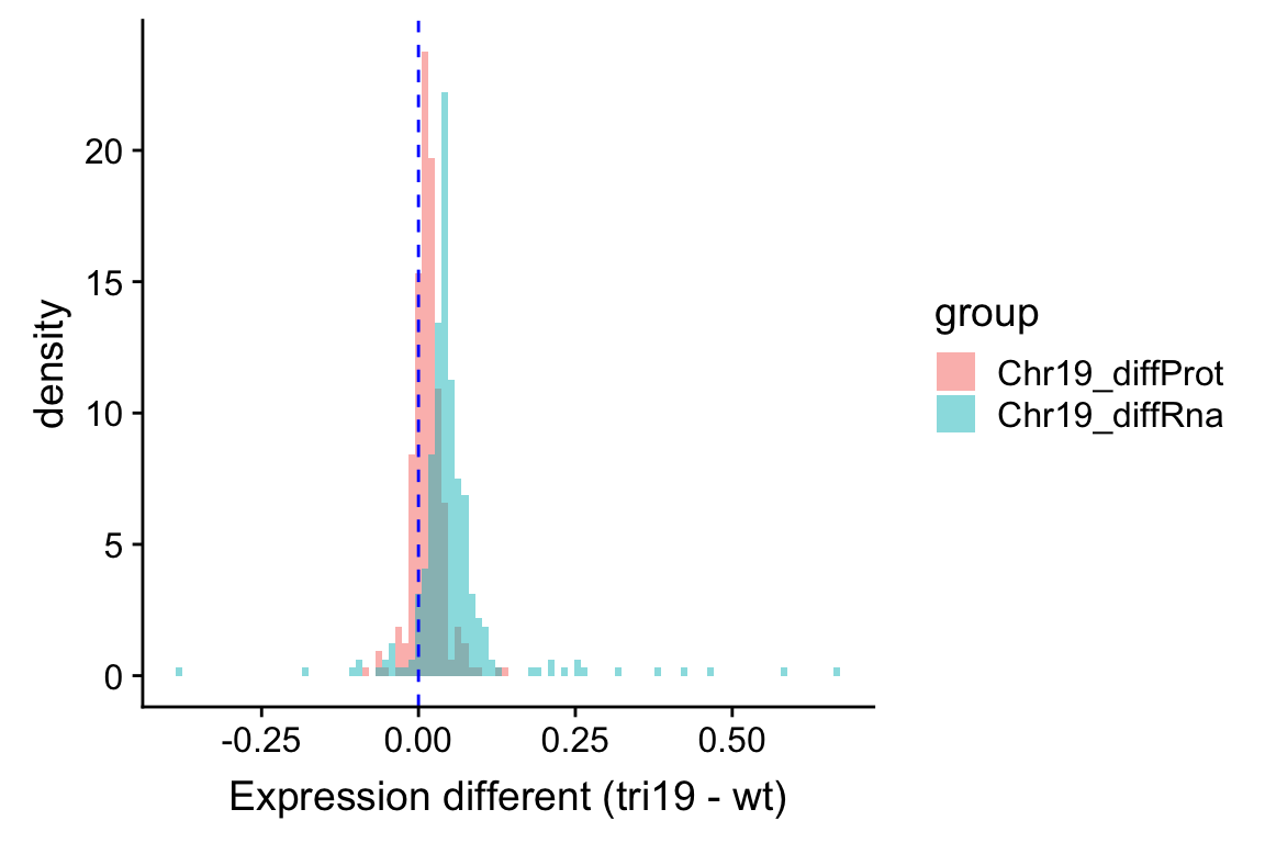 Similar as the plot above, it can be seen that RNA expression change is larger than the protein expression change. This also indicates a buffering effect. Although it’s not a complete buffering, as the average protein expression difference is still larger than 0.
Analysis of the buffering effect
Quantifying buffering effect by comparing magnitude of differential expression
Differential expression in proteomics
#subset samples
overSample <- intersect(dds$PatID, colnames(protCLL))
protSub <- protCLL[rowData(protCLL)$chromosome_name %in% "19",overSample]
overGene <- na.omit(intersect(rownames(dds),rowData(protSub)$ensembl_gene_id))
protSub <- protSub[rowData(protSub)$ensembl_gene_id %in% overGene, ]
rownames(protSub) <- rowData(protSub)$ensembl_gene_id
designMat <- data.frame(row.names = colnames(protSub),
                        trisomy19 = protSub$trisomy19)
exprMat <- assays(protSub)[["count"]]

#testing

fit <- proDA(exprMat, design = ~ ., col_data = designMat )

resTab.prot <- test_diff(fit, contrast = "trisomy191") %>%
  select(name, pval, diff, t_statistic, adj_pval) %>%
  dplyr::rename(id = name, logFC.prot = diff, stat.prot = t_statistic, pval.prot = pval, padj.prot = adj_pval)
Differential expression in RNAseq
#subset samples
overSample <- intersect(dds$PatID, colnames(protCLL))
ddsSub <- dds[overGene,overSample]
ddsSub$IGHV <- protSub[,ddsSub$PatID]$IGHV.status
ddsSub$trisomy19 <- protSub[,ddsSub$PatID]$trisomy19

design(ddsSub) <- ~ trisomy19
#testing
deRes <- DESeq(ddsSub)

resTab.rna <- results(deRes, name = "trisomy19_1_vs_0", tidy = TRUE) %>%
  select(row, log2FoldChange, stat, pvalue, padj) %>%
  dplyr::rename(id = row, logFC.rna = log2FoldChange, stat.rna = stat, pval.rna = pvalue, padj.rna = padj) %>%
  mutate(logFC.rna = logFC.rna*log(2)) #change to log fold change, same as proteomic
Define a buffering score
comTab <- left_join(resTab.prot, resTab.rna, by = "id") %>%
  mutate(symbol = rowData(dds[id,])$symbol)
Only chr19 genes that are up-regulated are considered. Otherwise it’s hard to intepret the dosage effect.
bufferTab <- comTab %>% filter(stat.rna > 0, stat.prot>0) %>%
  ungroup() %>%
  mutate(stat.prot.sqrt = sqrt(stat.prot),
         stat.prot.center = stat.prot.sqrt - mean(stat.prot.sqrt)) %>%
  mutate(diffStat = stat.rna-stat.prot,
         diffFold = logFC.rna -logFC.prot) %>%
  mutate(score = -stat.prot.center*stat.rna) %>%
  mutate(ifBuffer = case_when(
    padj.prot < 0.25 & padj.rna < 0.25 ~ "noBuffer",
    padj.prot > 0.25 & padj.rna < 0.25 ~ "Buffered",
    padj.prot < 0.25 & padj.rna > 0.25 ~ "Enhanced",
    TRUE ~ "undetermined"
  )) %>%
  arrange(desc(score))
Here I use two ways to quantify the buffering effect:
A buffering score, which is based on the difference of log fold change between protein and rna dataset and the t-statistics of the differentially expressed RNAs. The purpose is to give the gene that show significant and strong RNA change, but little protein change a high buffering score. While the genes that do not show strong RNA expression change will have a score close to zero. And the genes that show both strong protein and RNA expression change a more negative score.
A categorical variable, “ifBuffer”, based on the the significance of differential expression. The genes that show both significant protein and RNA up-regulation are in the “noBuffer” group, while the genes that show significant RNA-up-regulation but no significant protein expression change are in the “Buffered” group. The “Enhanced” group contains the genes that do not show significant changes in RNA level but with significant changes in protein level. The buffering score can not differentiate this group and will categorize it as undetermined. But the genes in this group, although pretty rare, may also be potentially interesting. Other genes are in the “undetermined” group.
Noted that here I use a less string FDR cut off (25%) than the cut-off used in trisomy12 analysis (10%). Because there are less samples here and if I still use 10% FDR, no differential expression related to trisomy19 will be detected
ggplot(bufferTab, aes(x=ifBuffer,y=score, fill = ifBuffer)) + geom_boxplot() + geom_point()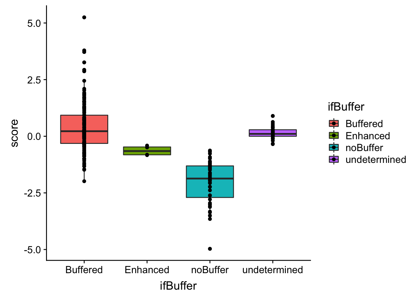 The buffering score and the categorical variable are related. Perhaps the buffering score can estimate more subtle effect, like the degree of buffering.
table(bufferTab$ifBuffer)
    Buffered     Enhanced     noBuffer undetermined
         153            4           43           27
Compare fold change in RNA expression and protein expression
ggplot(bufferTab, aes(x=logFC.rna, y=logFC.prot)) + geom_point(aes(col = ifBuffer)) +
  xlab("RNA log fold change") + ylab("Protein log fold change") +
geom_smooth(method = "lm") 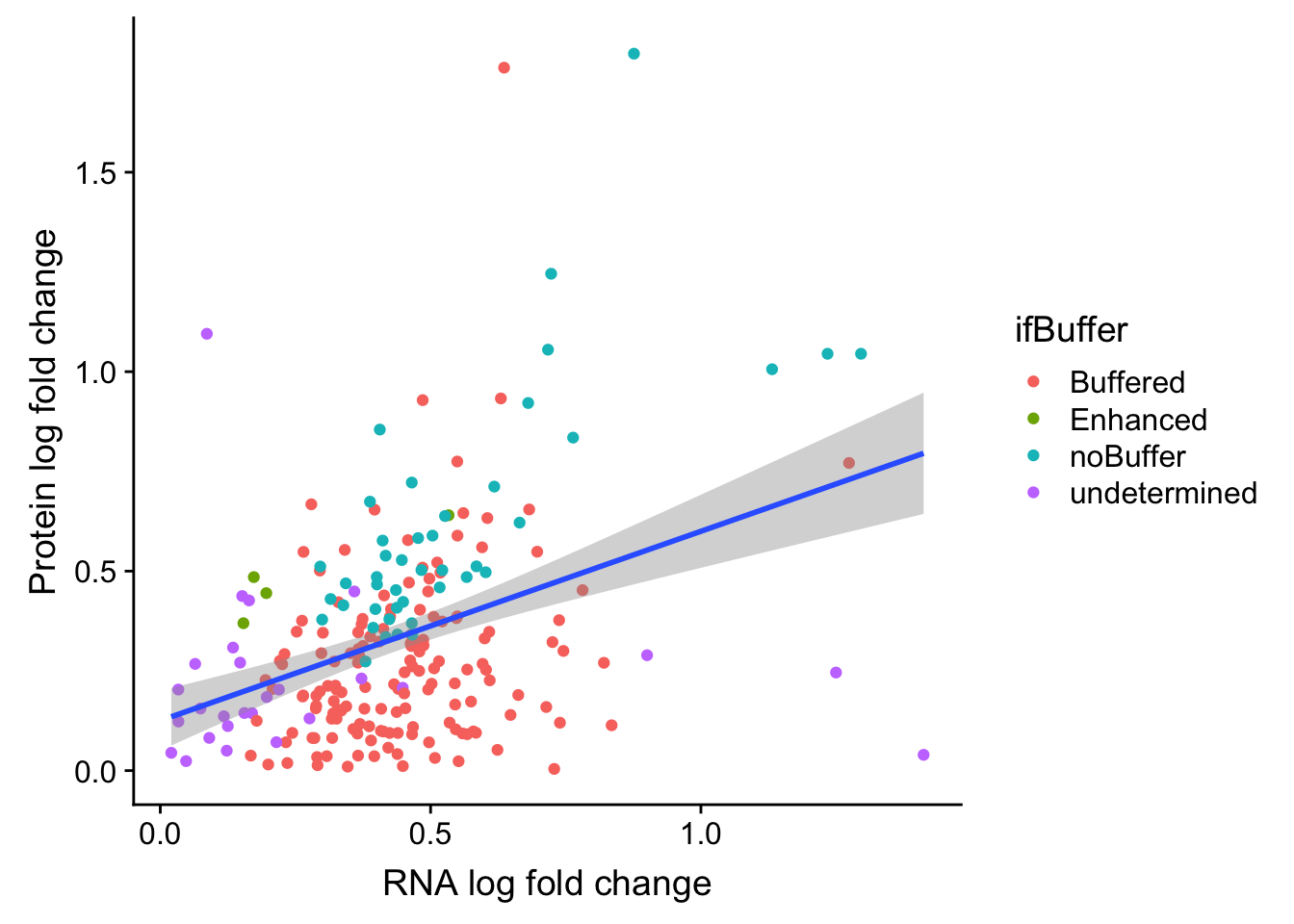
Table to show buffering effect
select(bufferTab, symbol, ifBuffer, score, padj.prot, padj.rna, logFC.prot,logFC.rna) %>%
  mutate_if(is.numeric, formatC, digits=2) %>%
DT::datatable()Plot most and least buffered genes
Top 9 most buffered based on buffering score
geneList <- bufferTab$id[1:9]
pList <- lapply(geneList, function(i) {
  tabProt <- allProtTab %>% filter(id == i) %>%
    select(id, patID, symbol,expr) %>% dplyr::rename(protExpr = expr)
  tabRna <- allRnaTab %>% filter(id == i) %>%
    select(id, patID, expr) %>% dplyr::rename(rnaExpr = expr)
  plotTab <- left_join(tabProt, tabRna, by = c("id","patID")) %>%
    filter(!is.na(protExpr), !is.na(rnaExpr)) %>%
    mutate(trisomy19 = patMeta[match(patID, patMeta$Patient.ID),]$trisomy19)
  p <- ggplot(plotTab, aes(x=rnaExpr, y = protExpr)) +
    geom_point(aes(col=trisomy19)) + geom_smooth(method="lm") + ggtitle(unique(plotTab$symbol)) +
    theme(legend.position = "bottom")
  ggMarginal(p, type = "histogram", groupFill = TRUE)
  })
cowplot::plot_grid(plotlist = pList, ncol=3)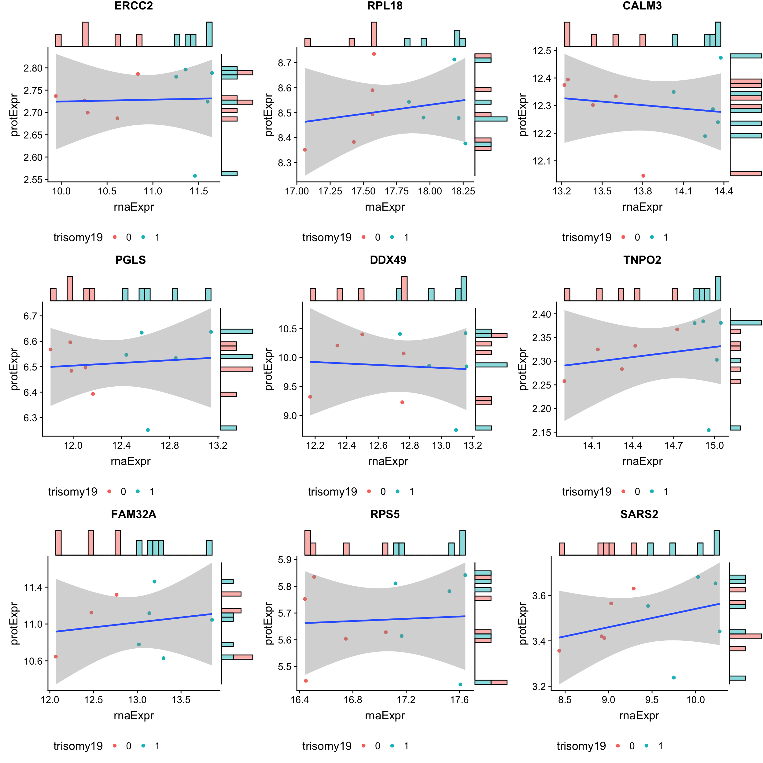
The 9 least buffered based on buffering score
geneList <- tail(bufferTab$id, n=9)
pList <- lapply(geneList, function(i) {
  tabProt <- allProtTab %>% filter(id == i) %>%
    select(id, patID, symbol,expr) %>% dplyr::rename(protExpr = expr)
  tabRna <- allRnaTab %>% filter(id == i) %>%
    select(id, patID, expr) %>% dplyr::rename(rnaExpr = expr)
  plotTab <- left_join(tabProt, tabRna, by = c("id","patID")) %>%
    filter(!is.na(protExpr), !is.na(rnaExpr)) %>%
    mutate(trisomy19 = patMeta[match(patID, patMeta$Patient.ID),]$trisomy19)
  p <- ggplot(plotTab, aes(x=rnaExpr, y = protExpr)) +
    geom_point(aes(col=trisomy19)) + geom_smooth(method="lm") +
    ggtitle(unique(plotTab$symbol)) +
    theme(legend.position = "bottom")
  ggMarginal(p, type = "histogram", groupFill = TRUE)
  })
cowplot::plot_grid(plotlist = pList, ncol=3)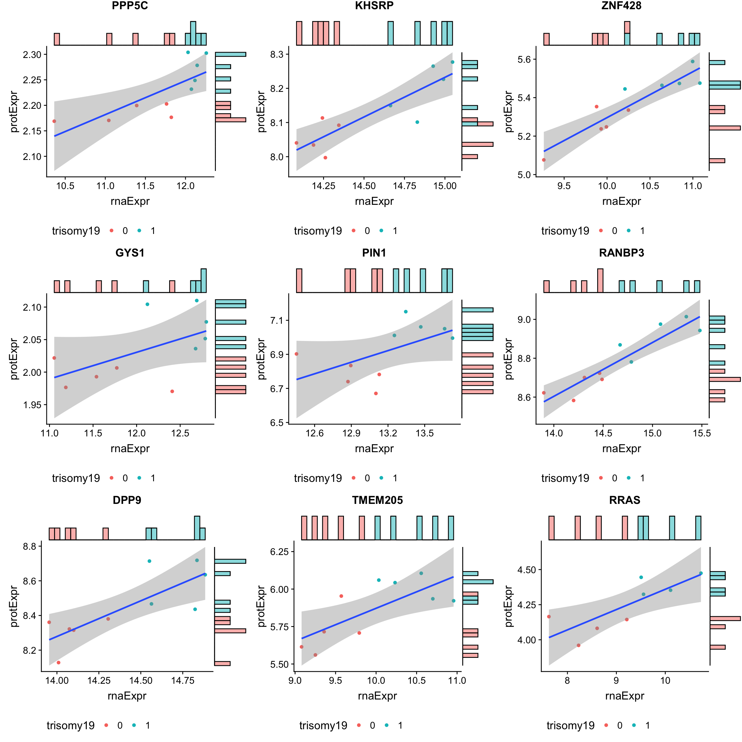
Plot the 4 genes in the enhanced group, where protein change is more significant than RNA change
geneList <- filter(bufferTab, ifBuffer == "Enhanced")$id
pList <- lapply(geneList, function(i) {
  tabProt <- allProtTab %>% filter(id == i) %>%
    select(id, patID, symbol,expr) %>% dplyr::rename(protExpr = expr)
  tabRna <- allRnaTab %>% filter(id == i) %>%
    select(id, patID, expr) %>% dplyr::rename(rnaExpr = expr)
  plotTab <- left_join(tabProt, tabRna, by = c("id","patID")) %>%
    filter(!is.na(protExpr), !is.na(rnaExpr)) %>%
    mutate(trisomy19 = patMeta[match(patID, patMeta$Patient.ID),]$trisomy19)
  p <- ggplot(plotTab, aes(x=rnaExpr, y = protExpr)) +
    geom_point(aes(col=trisomy19)) + geom_smooth(method="lm") +
    ggtitle(unique(plotTab$symbol)) +
    theme(legend.position = "bottom")
  ggMarginal(p, type = "histogram", groupFill = TRUE)
  })
cowplot::plot_grid(plotlist = pList, ncol=2)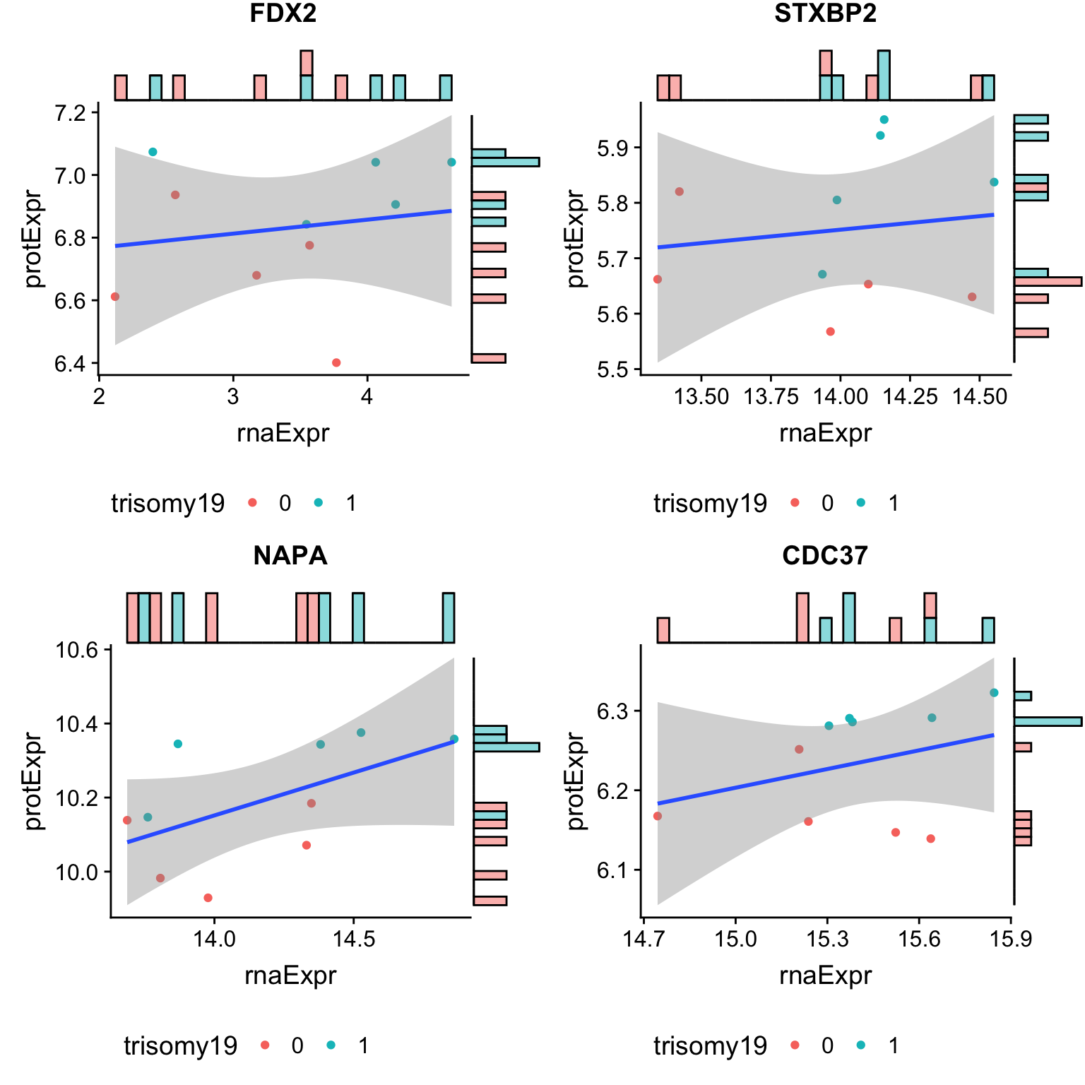
Enrichment analysis based on buffering score
inputTab <- bufferTab %>% select(symbol, score) %>%
  arrange(abs(score)) %>% distinct(symbol, .keep_all = T) %>%
  data.frame() %>% column_to_rownames("symbol")

gmts = list(H= "../data/gmts/h.all.v6.2.symbols.gmt",
            KEGG = "../data/gmts/c2.cp.kegg.v6.2.symbols.gmt")
enRes <- list()
enRes[["HALLMARK"]] <- jyluMisc::runGSEA(inputTab, gmts$H, "page")
enRes[["KEGG"]] <- jyluMisc::runGSEA(inputTab, gmts$KEGG, "page")
p <- jyluMisc::plotEnrichmentBar(enRes, pCut =0.05, ifFDR= FALSE)
#pdf("tri19Enrich.pdf", height = 15, width = 6)
plot(p)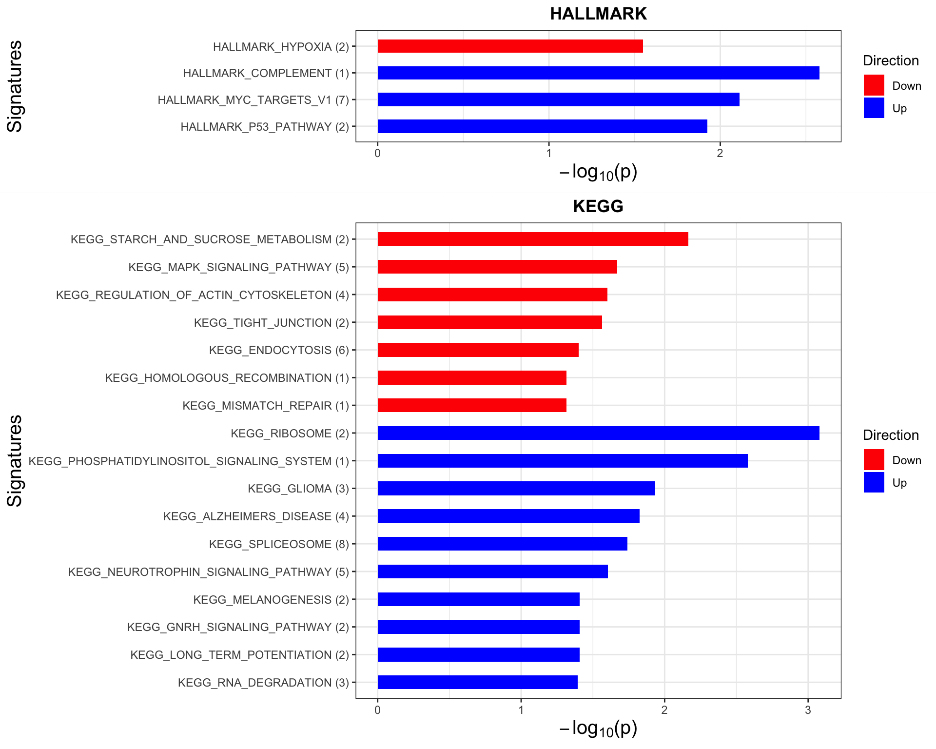
#dev.off()Here, down indicate the pathways that the non-buffered proteins are enrichment. Up indicates the pathways that the buffered proteins are enriched
Whether buffering is related to protein complexes
int_pairs = read_delim("../data/proteins_in_complexes", delim = "\t") %>%
  mutate(symbolA = rowData(protCLL)[match(ProtA, rownames(protCLL)),]$hgnc_symbol,
         symbolB = rowData(protCLL)[match(ProtB, rownames(protCLL)),]$hgnc_symbol) %>%
  filter(!is.na(symbolA),!is.na(symbolB))
bufferTab <- mutate(bufferTab, inComplex = ifelse(symbol %in% c(int_pairs$symbolA, int_pairs$symbolB), TRUE, FALSE))Plot the buffering scores of proteins in complex and not in complex
ggplot(bufferTab, aes(x=inComplex, y=score)) + geom_boxplot() + geom_point()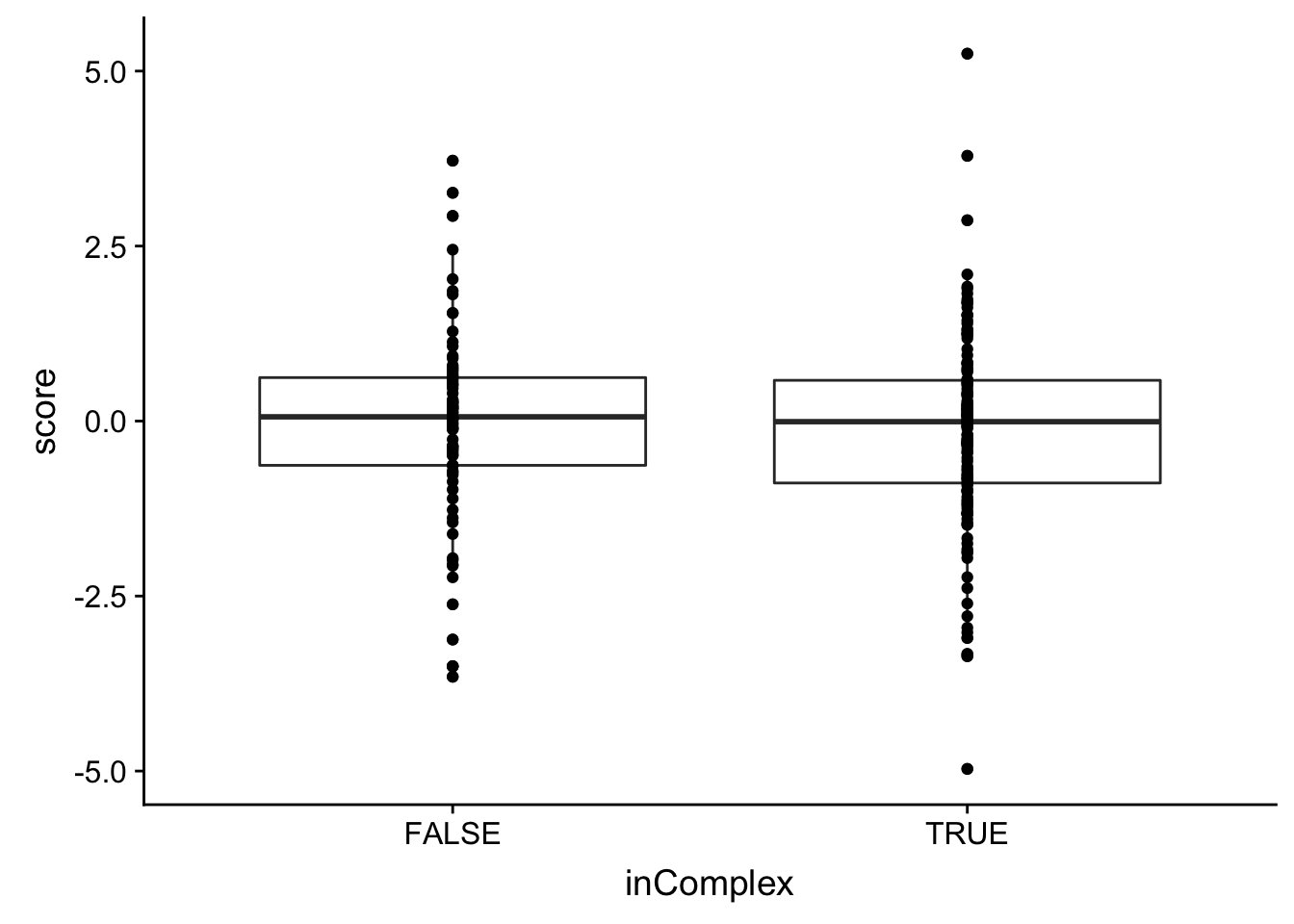
t.test(score~inComplex, bufferTab, var.equal= TRUE)
    Two Sample t-test

data:  score by inComplex
t = 0.34108, df = 225, p-value = 0.7334
alternative hypothesis: true difference in means is not equal to 0
95 percent confidence interval:
 -0.3094802  0.4390418
sample estimates:
mean in group FALSE  mean in group TRUE
        -0.06606103         -0.13084183
No significant differences can be observed.
There’s not significant associations between whether the protein is in complex and whether the protein expression is buffered.
Plot buffering effect on genomic coordinates
plotFoldGenome <- function(bufferTab, allBand, allProtTab, chr, region = c(-Inf,Inf),
                           ifTrend = FALSE, maxVal =1, minVal=-1) {

  #table for cyto band
  bandTab <- filter(allBand, ChromID == chr, chromStart >= region[1], chromEnd <= region[2]) %>%
    mutate(chromMid = chromMid)

  #table for fold change
  protCoordTab <- allProtTab %>% distinct(symbol, start_position, end_position, mid_position)
  foldTab <- bufferTab %>% select(symbol, logFC.prot, logFC.rna, score, ifBuffer) %>%
    gather(key = "set", value = "logFC", -symbol, -score,-ifBuffer) %>%
    left_join(protCoordTab)
  bufferLine <- filter(bufferTab, ifBuffer %in% c("Buffered","Enhanced")) %>%
    left_join(protCoordTab) %>%
    distinct(symbol, mid_position, logFC.prot, logFC.rna, ifBuffer) %>%
    mutate(minY = ifelse(logFC.prot > logFC.rna, logFC.rna, logFC.prot),
           maxY= ifelse(logFC.prot > logFC.rna, logFC.prot, logFC.rna))

  xMax <- max(bandTab$chromEnd, na.rm = T)

  #main plot for Protein
  gPro <- ggplot() +
    geom_rect(data=bandTab, mapping=aes(xmin=chromStart, xmax=chromEnd, ymin=minVal, ymax=maxVal,
                                        fill=Colour, label = band), alpha=0.1) +
    geom_text(data=bandTab, mapping=aes(label=band, x=chromMid), y=maxVal, hjust =1, angle = 90, size=2.5) +
    geom_rect(data = foldTab,
            mapping=aes(xmin=start_position,
                        xmax=end_position, ymin=logFC, ymax=logFC+0.1,
                        fill = set)) +
    geom_segment(data = bufferLine, aes(x=mid_position, xend = mid_position,
                                        y=minY + 0.1, yend = maxY, col = ifBuffer),
                 linetype = "dashed") +
    scale_x_continuous(expand=c(0,0),limits = c(0,xMax)) +
    xlab("Genomic position [Mb]") +
    ylab("Log Fold Change") +
    scale_fill_manual(values = c(even = "white",odd = "grey50",
                                logFC.rna = "orange", logFC.prot = "darkblue")) +
    scale_color_manual(values = c(logFC.rna = "orange",logFC.prot = "darkblue",
                                  Buffered = "red",Enhanced = "green")) +
    ggtitle(paste0("Log fold change comparison","(",chr,")")) +
    ggrepel::geom_text_repel(data = bufferLine,
                                 aes(x=mid_position, y=logFC.prot, label = symbol, col = ifBuffer)) +
    theme(plot.title = element_text(face = "bold", size = 10, hjust = 0.3),
        legend.position = "none",
        panel.background = element_blank(),
        panel.grid.major = element_line(colour="grey90", size=0.1))

    if (ifTrend) {
      gPro <- gPro + stat_smooth(data =foldTab, geom="line",
                mapping = aes(y=logFC, x= mid_position,
                              color = set),
                formula = y ~ x, method = "loess", se=FALSE, span=0.2,
                size =0.5, alpha=0.5)
    }


    #for legend
    ## if the patient has CNV data
    lgTab <- tibble(x= seq(6),y=seq(6),
                    Dataset = c(rep("logFC.rna",3), rep("logFC.prot",3)),
                    ifBuffer = c(rep("Buffered",3), rep("Enhanced",3)))

    lg <- ggplot(lgTab, aes(x=x,y=y)) +
      geom_point(aes(fill = Dataset, color = ifBuffer), shape =22,size=3) +
      scale_fill_manual(values = c(logFC.rna = "orange", logFC.prot = "darkblue")) +
      scale_color_manual(values = c(logFC.rna = "orange",logFC.prot = "darkblue",
                                  Buffered = "red",Enhanced = "green")) +
      theme(legend.position = "bottom")

    lg <- get_legend(lg)

    return(list(plot = gPro, legend = lg))
}
g <- plotFoldGenome(bufferTab, allBand, allProtTab, "chr19", region = c(-Inf,Inf),
ifTrend = TRUE, maxVal =2, minVal=0)
pg <- plot_grid(g$plot, g$legend, ncol = 1, rel_heights = c(1,0.1))
pg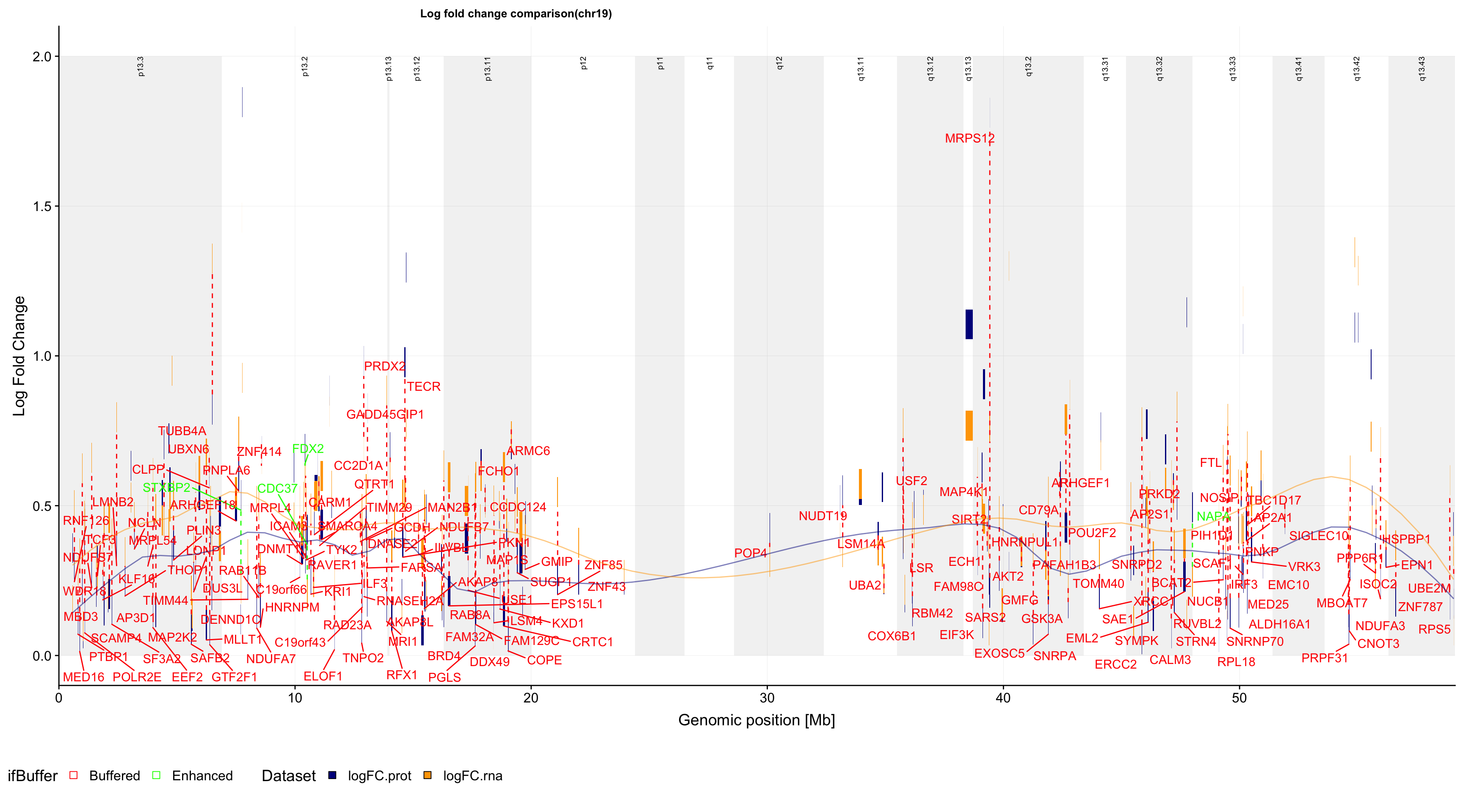
ggsave(filename = "../public/trisomy19_buffer_plot.pdf", plot = pg, device = "pdf", height = 10, width = 18)PDF version: trisomy19_buffer_plot.pdf
In this plot, the y axis in the log fold change of either protein (blue) or RNA (orange) expression (trisomy19 vs WT). If there’s a “Buffering” effect, the protein and rna is connected by a red dotted line. If there’s an “Enhanced” effect, they will be joined by a green dotted line.
Summary:
Similar as trisomy12, the gene dosage effect of trisomy19 is visible in both RNA expression and protein expression, as compared to WT samples, the genes on Chr19 show elevated global expression of both RNA and protein in trisomy19 sample. But the scale of difference is less in proteins and the protein expression is less varied than RNA expression. This may be due to the buffering or moderation effect of translation or some other mechanisms that regulate protein abundance.
The buffering effect seems to be stronger in trisomy19 than trisomy12. But it’s difficult to compare as there’s large sample size difference and therefore differences in statistical power.
Same as trisomy12, there’s no significant association between the buffering effect and whether the protein is in complex or not.
sessionInfo()R version 3.6.0 (2019-04-26)
Platform: x86_64-apple-darwin15.6.0 (64-bit)
Running under: macOS 10.15.4
Matrix products: default
BLAS: /Library/Frameworks/R.framework/Versions/3.6/Resources/lib/libRblas.0.dylib
LAPACK: /Library/Frameworks/R.framework/Versions/3.6/Resources/lib/libRlapack.dylib
locale:
[1] en_US.UTF-8/en_US.UTF-8/en_US.UTF-8/C/en_US.UTF-8/en_US.UTF-8
attached base packages:
[1] parallel stats4 stats graphics grDevices utils datasets
[8] methods base
other attached packages:
[1] forcats_0.4.0 stringr_1.4.0
[3] dplyr_0.8.5 purrr_0.3.3
[5] readr_1.3.1 tidyr_1.0.0
[7] tibble_3.0.0 tidyverse_1.3.0
[9] cowplot_0.9.4 ggplot2_3.3.0
[11] ggExtra_0.9 proDA_1.1.2
[13] jyluMisc_0.1.5 piano_2.0.2
[15] DESeq2_1.24.0 SummarizedExperiment_1.14.0
[17] DelayedArray_0.10.0 BiocParallel_1.18.0
[19] matrixStats_0.54.0 Biobase_2.44.0
[21] GenomicRanges_1.36.0 GenomeInfoDb_1.20.0
[23] IRanges_2.18.1 S4Vectors_0.22.0
[25] BiocGenerics_0.30.0
loaded via a namespace (and not attached):
[1] readxl_1.3.1 backports_1.1.4 Hmisc_4.2-0
[4] fastmatch_1.1-0 drc_3.0-1 workflowr_1.6.0
[7] igraph_1.2.4.1 shinydashboard_0.7.1 splines_3.6.0
[10] crosstalk_1.0.0 TH.data_1.0-10 digest_0.6.19
[13] htmltools_0.4.0 gdata_2.18.0 magrittr_1.5
[16] checkmate_2.0.0 memoise_1.1.0 cluster_2.1.0
[19] openxlsx_4.1.0.1 limma_3.40.2 annotate_1.62.0
[22] modelr_0.1.5 sandwich_2.5-1 colorspace_1.4-1
[25] ggrepel_0.8.1 rvest_0.3.5 blob_1.1.1
[28] haven_2.2.0 xfun_0.8 crayon_1.3.4
[31] RCurl_1.95-4.12 jsonlite_1.6 genefilter_1.66.0
[34] survival_2.44-1.1 zoo_1.8-6 glue_1.3.2
[37] survminer_0.4.4 gtable_0.3.0 zlibbioc_1.30.0
[40] XVector_0.24.0 car_3.0-3 abind_1.4-5
[43] scales_1.1.0 mvtnorm_1.0-11 DBI_1.0.0
[46] relations_0.6-8 miniUI_0.1.1.1 Rcpp_1.0.1
[49] plotrix_3.7-6 cmprsk_2.2-8 xtable_1.8-4
[52] htmlTable_1.13.1 foreign_0.8-71 bit_1.1-14
[55] km.ci_0.5-2 Formula_1.2-3 DT_0.7
[58] httr_1.4.1 htmlwidgets_1.3 fgsea_1.10.0
[61] gplots_3.0.1.1 RColorBrewer_1.1-2 acepack_1.4.1
[64] ellipsis_0.2.0 farver_2.0.3 pkgconfig_2.0.2
[67] XML_3.98-1.20 dbplyr_1.4.2 nnet_7.3-12
[70] locfit_1.5-9.1 labeling_0.3 tidyselect_1.0.0
[73] rlang_0.4.5 later_0.8.0 AnnotationDbi_1.46.0
[76] munsell_0.5.0 cellranger_1.1.0 tools_3.6.0
[79] visNetwork_2.0.7 cli_1.1.0 generics_0.0.2
[82] RSQLite_2.1.1 broom_0.5.2 evaluate_0.14
[85] yaml_2.2.0 knitr_1.23 bit64_0.9-7
[88] fs_1.4.0 zip_2.0.2 survMisc_0.5.5
[91] caTools_1.17.1.2 nlme_3.1-140 mime_0.7
[94] slam_0.1-45 xml2_1.2.2 compiler_3.6.0
[97] rstudioapi_0.10 curl_3.3 ggsignif_0.5.0
[100] marray_1.62.0 reprex_0.3.0 geneplotter_1.62.0
[103] stringi_1.4.3 lattice_0.20-38 Matrix_1.2-17
[106] KMsurv_0.1-5 shinyjs_1.0 vctrs_0.2.4
[109] pillar_1.4.3 lifecycle_0.2.0 data.table_1.12.2
[112] bitops_1.0-6 httpuv_1.5.1 extraDistr_1.8.11
[115] R6_2.4.0 latticeExtra_0.6-28 promises_1.0.1
[118] KernSmooth_2.23-15 gridExtra_2.3 rio_0.5.16
[121] codetools_0.2-16 MASS_7.3-51.4 gtools_3.8.1
[124] exactRankTests_0.8-30 assertthat_0.2.1 rprojroot_1.3-2
[127] withr_2.1.2 multcomp_1.4-10 GenomeInfoDbData_1.2.1
[130] mgcv_1.8-28 hms_0.5.2 grid_3.6.0
[133] rpart_4.1-15 rmarkdown_1.13 carData_3.0-2
[136] ggpubr_0.2.1 git2r_0.26.1 maxstat_0.7-25
[139] sets_1.0-18 lubridate_1.7.4 shiny_1.3.2
[142] base64enc_0.1-3