Protein markers for drug responses (1000CPS)
Junyan Lu
2020-06-08
Last updated: 2020-06-16
Checks: 5 2
Knit directory: Proteomics/analysis/
This reproducible R Markdown analysis was created with workflowr (version 1.6.0). The Checks tab describes the reproducibility checks that were applied when the results were created. The Past versions tab lists the development history.
The R Markdown is untracked by Git. To know which version of the R Markdown file created these results, you’ll want to first commit it to the Git repo. If you’re still working on the analysis, you can ignore this warning. When you’re finished, you can run wflow_publish to commit the R Markdown file and build the HTML.
Great job! The global environment was empty. Objects defined in the global environment can affect the analysis in your R Markdown file in unknown ways. For reproduciblity it’s best to always run the code in an empty environment.
The command set.seed(20200227) was run prior to running the code in the R Markdown file. Setting a seed ensures that any results that rely on randomness, e.g. subsampling or permutations, are reproducible.
Great job! Recording the operating system, R version, and package versions is critical for reproducibility.
- unnamed-chunk-10
- unnamed-chunk-12
- unnamed-chunk-15
- unnamed-chunk-17
- unnamed-chunk-20
- unnamed-chunk-22
- unnamed-chunk-5
- unnamed-chunk-7
To ensure reproducibility of the results, delete the cache directory analysisDrugResponses_cache and re-run the analysis. To have workflowr automatically delete the cache directory prior to building the file, set delete_cache = TRUE when running wflow_build() or wflow_publish().
Great job! Using relative paths to the files within your workflowr project makes it easier to run your code on other machines.
Great! You are using Git for version control. Tracking code development and connecting the code version to the results is critical for reproducibility. The version displayed above was the version of the Git repository at the time these results were generated.
Note that you need to be careful to ensure that all relevant files for the analysis have been committed to Git prior to generating the results (you can use wflow_publish or wflow_git_commit). workflowr only checks the R Markdown file, but you know if there are other scripts or data files that it depends on. Below is the status of the Git repository when the results were generated:
Ignored files:
    Ignored:    .DS_Store
    Ignored:    .Rhistory
    Ignored:    .Rproj.user/
    Ignored:    analysis/.DS_Store
    Ignored:    analysis/.Rhistory
    Ignored:    analysis/analysisDrugResponses_IC50_cache/
    Ignored:    analysis/analysisDrugResponses_cache/
    Ignored:    analysis/complexAnalysis_IGHV_alternative_cache/
    Ignored:    analysis/complexAnalysis_IGHV_cache/
    Ignored:    analysis/complexAnalysis_trisomy12_alteredPQR_cache/
    Ignored:    analysis/complexAnalysis_trisomy12_alternative_cache/
    Ignored:    analysis/complexAnalysis_trisomy12_cache/
    Ignored:    analysis/correlateCLLPD_cache/
    Ignored:    analysis/predictOutcome_cache/
    Ignored:    code/.Rhistory
    Ignored:    data/.DS_Store
    Ignored:    output/.DS_Store

Untracked files:
    Untracked:  analysis/CNVanalysis_11q.Rmd
    Untracked:  analysis/CNVanalysis_trisomy12.Rmd
    Untracked:  analysis/CNVanalysis_trisomy19.Rmd
    Untracked:  analysis/analysisDrugResponses.Rmd
    Untracked:  analysis/analysisDrugResponses_IC50.Rmd
    Untracked:  analysis/analysisPCA.Rmd
    Untracked:  analysis/analysisSplicing.Rmd
    Untracked:  analysis/analysisTrisomy19.Rmd
    Untracked:  analysis/annotateCNV.Rmd
    Untracked:  analysis/complexAnalysis_IGHV.Rmd
    Untracked:  analysis/complexAnalysis_IGHV_alternative.Rmd
    Untracked:  analysis/complexAnalysis_overall.Rmd
    Untracked:  analysis/complexAnalysis_trisomy12.Rmd
    Untracked:  analysis/complexAnalysis_trisomy12_alternative.Rmd
    Untracked:  analysis/correlateGenomic_PC12adjusted.Rmd
    Untracked:  analysis/correlateGenomic_noBlock.Rmd
    Untracked:  analysis/correlateGenomic_noBlock_MCLL.Rmd
    Untracked:  analysis/correlateGenomic_noBlock_UCLL.Rmd
    Untracked:  analysis/correlateRNAexpression.Rmd
    Untracked:  analysis/default.css
    Untracked:  analysis/del11q.pdf
    Untracked:  analysis/del11q_norm.pdf
    Untracked:  analysis/peptideValidate.Rmd
    Untracked:  analysis/plotExpressionCNV.Rmd
    Untracked:  analysis/processPeptides_LUMOS.Rmd
    Untracked:  analysis/style.css
    Untracked:  analysis/trisomy12.pdf
    Untracked:  analysis/trisomy12_AFcor.Rmd
    Untracked:  analysis/trisomy12_norm.pdf
    Untracked:  code/AlteredPQR.R
    Untracked:  code/utils.R
    Untracked:  data/190909_CLL_prot_abund_med_norm.tsv
    Untracked:  data/190909_CLL_prot_abund_no_norm.tsv
    Untracked:  data/20190423_Proteom_submitted_samples_bereinigt.xlsx
    Untracked:  data/20191025_Proteom_submitted_samples_final.xlsx
    Untracked:  data/LUMOS/
    Untracked:  data/LUMOS_peptides/
    Untracked:  data/LUMOS_protAnnotation.csv
    Untracked:  data/LUMOS_protAnnotation_fix.csv
    Untracked:  data/SampleAnnotation_cleaned.xlsx
    Untracked:  data/example_proteomics_data
    Untracked:  data/facTab_IC50atLeast3New.RData
    Untracked:  data/gmts/
    Untracked:  data/mapEnsemble.txt
    Untracked:  data/mapSymbol.txt
    Untracked:  data/proteins_in_complexes
    Untracked:  data/pyprophet_export_aligned.csv
    Untracked:  data/timsTOF_protAnnotation.csv
    Untracked:  output/LUMOS_processed.RData
    Untracked:  output/cnv_plots.zip
    Untracked:  output/cnv_plots/
    Untracked:  output/cnv_plots_norm.zip
    Untracked:  output/dxdCLL.RData
    Untracked:  output/exprCNV.RData
    Untracked:  output/lassoResults_CPS.RData
    Untracked:  output/lassoResults_IC50.RData
    Untracked:  output/pepCLL_lumos.RData
    Untracked:  output/pepTab_lumos.RData
    Untracked:  output/plotCNV_allChr11_diff.pdf
    Untracked:  output/plotCNV_del11q_sum.pdf
    Untracked:  output/proteomic_LUMOS_20200227.RData
    Untracked:  output/proteomic_LUMOS_20200320.RData
    Untracked:  output/proteomic_LUMOS_20200430.RData
    Untracked:  output/proteomic_timsTOF_20200227.RData
    Untracked:  output/splicingResults.RData
    Untracked:  output/timsTOF_processed.RData
    Untracked:  plotCNV_del11q_diff.pdf

Unstaged changes:
    Modified:   analysis/_site.yml
    Modified:   analysis/analysisSF3B1.Rmd
    Modified:   analysis/compareProteomicsRNAseq.Rmd
    Modified:   analysis/correlateCLLPD.Rmd
    Modified:   analysis/correlateGenomic.Rmd
    Deleted:    analysis/correlateGenomic_removePC.Rmd
    Modified:   analysis/correlateMIR.Rmd
    Modified:   analysis/correlateMethylationCluster.Rmd
    Modified:   analysis/index.Rmd
    Modified:   analysis/predictOutcome.Rmd
    Modified:   analysis/processProteomics_LUMOS.Rmd
    Modified:   analysis/qualityControl_LUMOS.Rmd
Note that any generated files, e.g. HTML, png, CSS, etc., are not included in this status report because it is ok for generated content to have uncommitted changes.
There are no past versions. Publish this analysis with wflow_publish() to start tracking its development.
Correlations between protein abundance and drug response
Preprocess datasets
Drug screening data from 1000CPS: low quality samples after QC are removed; the edge effect corrected viability values are used
viabMat.auc <- pheno1000_main %>% filter(!lowQuality, ! Drug %in% c("DMSO","PBS"), patientID %in% colnames(protCLL)) %>%
  group_by(patientID, Drug) %>% summarise(viab = mean(normVal.adj.cor_auc)) %>%
  spread(key = patientID, value = viab) %>%
  data.frame(stringsAsFactors = FALSE) %>% column_to_rownames("Drug") %>%
  as.matrix()

viabMat <- pheno1000_main %>% filter(!lowQuality, ! Drug %in% c("DMSO","PBS"), patientID %in% colnames(protCLL)) %>%
  group_by(patientID, Drug, concIndex) %>% summarise(viab = mean(normVal.adj.sigm)) %>% ungroup() %>%
  spread(key = patientID, value = viab) %>%
  mutate(drugConc = paste0(Drug, "_",concIndex)) %>% select(-Drug, -concIndex) %>%
  data.frame(stringsAsFactors = FALSE) %>% column_to_rownames("drugConc") %>%
  as.matrix()
Proteomics data
proMat <- assays(protCLL)[["count"]]
proMat <- proMat[,colnames(viabMat)]
Remove proteins without much variance (to lower multi-testing burden)
sds <- genefilter::rowSds(proMat,na.rm=TRUE)
proMat <- proMat[sds > genefilter::shorth(sds),]
Remove drugs without much variance (only for individual concentrations)
#individual concentrations
sds <- genefilter::rowSds(viabMat)
viabMat <- viabMat[sds > genefilter::shorth(sds),]
How many samples have both proteomics data and CPS1000 screen data
ncol(proMat)[1] 45Association test without any blocking
For individual concentrations
Association test
resTab <- lapply(rownames(viabMat),function(drugName) {
  viab <- viabMat[drugName, ]
  designMat <- model.matrix(~1+viab)
  fit <- lmFit(proMat,  designMat)
  fit2 <- eBayes(fit)
  corRes <- topTable(fit2, number ="all", adjust.method = "BH", coef = "viab") %>% rownames_to_column("id") %>%
    mutate(symbol = rowData(protCLL[id,])$hgnc_symbol, drugConc = drugName)
}) %>% bind_rows() %>% separate(drugConc, c("Drug","concIndex"),"_",remove = FALSE) %>%
  mutate(adj.P.Val = p.adjust(P.Value, method = "BH")) %>% arrange(P.Value)
Number of associations (10% FDR)
Select significant associations (10% FDR)
resTab.sig <- filter(resTab, adj.P.Val < 0.1) %>%
  select(Drug, symbol, id,logFC, P.Value, adj.P.Val, concIndex)
plotTab <- resTab.sig %>% group_by(Drug, concIndex) %>%
summarise(n = length(id)) %>% ungroup()
ordTab <- group_by(plotTab, Drug) %>% summarise(total = sum(n)) %>%
arrange(desc(total))
plotTab <- mutate(plotTab, Drug = factor(Drug, levels = ordTab$Drug)) %>%
filter(n>0)
ggplot(plotTab, aes(x=Drug,y=n,fill = concIndex)) + geom_bar(stat = "identity") +
theme(axis.text.x = element_text(angle = 90,hjust=1,vjust=0.5)) +
ylab("Number of associations") + xlab("")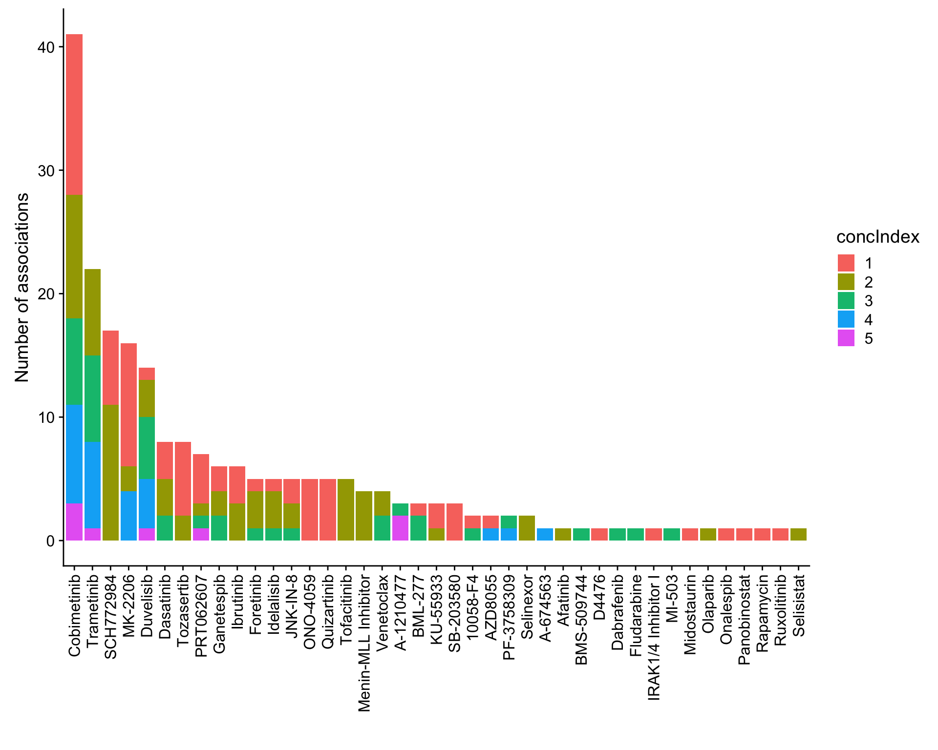
Table of significant associations (10% FDR)
resTab.sig %>% mutate_if(is.numeric, formatC, digits=2, format= "e") %>%
  DT::datatable()
Plot top 9 drug-protein associations
plotList <- lapply(seq(9), function(i) {
drugConc <- paste0(resTab.sig$Drug[i],"_",resTab.sig$concIndex[i])
proteinName <- resTab.sig$symbol[i]
id <- resTab.sig$id[i]
plotTab <- tibble(patID = colnames(viabMat),
viab = viabMat[drugConc,],
expr = proMat[id,]) %>%
mutate(IGHV = protCLL[,patID]$IGHV.status,
trisomy12 = protCLL[,patID]$trisomy12)
ggplot(plotTab, aes(x=viab, y=expr)) + geom_point(aes(col = trisomy12, shape = IGHV)) +
scale_shape_manual(values = c(M = 19, U = 1)) + geom_smooth(method = "lm", se=FALSE) +
ggtitle(sprintf("%s ~ %s", drugConc, proteinName)) +
ylab("Protein expression") + xlab("Viability after treatment") +
theme(legend.position = "bottom")
})
plot_grid(plotlist = plotList, ncol =3)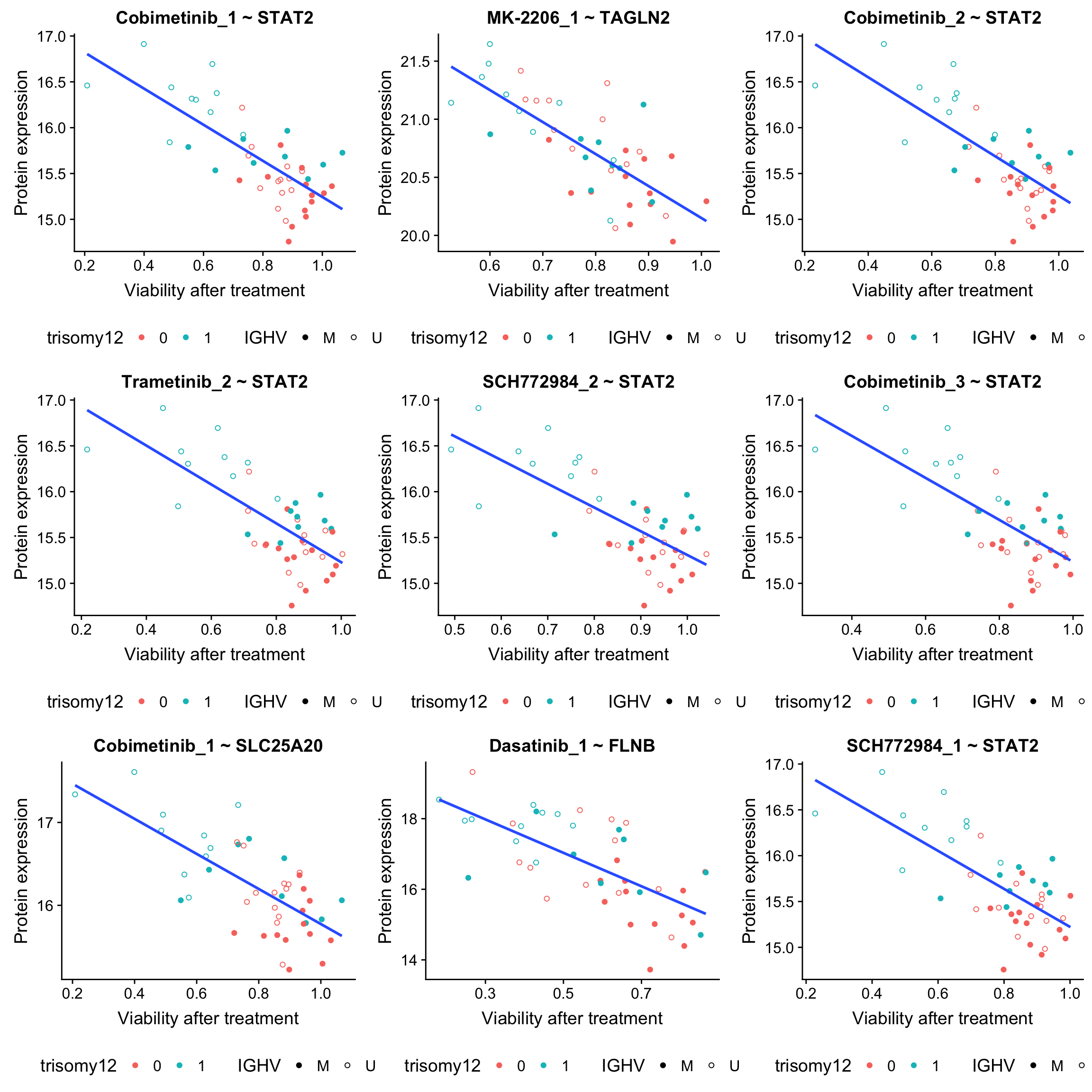 From those plots, it can be seen that those associations are potentially confounded by IGHV status and/or trisomy12.
For averaged five concentrations (AUC)
Association test
resTab.auc <- lapply(rownames(viabMat.auc),function(drugName) {
  viab <- viabMat.auc[drugName, ]
  designMat <- model.matrix(~1+viab)
  fit <- lmFit(proMat,  designMat)
  fit2 <- eBayes(fit)
  corRes <- topTable(fit2, number ="all", adjust.method = "BH", coef = "viab") %>% rownames_to_column("id") %>%
    mutate(symbol = rowData(protCLL[id,])$hgnc_symbol, Drug = drugName)
}) %>% bind_rows() %>% mutate(adj.P.Val = p.adjust(P.Value, method = "BH")) %>% arrange(P.Value)
Number of associations (10% FDR)
Select significant associations (10% FDR)
resTab.sig <- filter(resTab.auc, adj.P.Val < 0.1) %>%
  select(Drug, symbol, id,logFC, P.Value, adj.P.Val)
plotTab <- resTab.sig %>% group_by(Drug) %>%
summarise(n = length(id)) %>% ungroup()
ordTab <- group_by(plotTab, Drug) %>% summarise(total = sum(n)) %>%
arrange(desc(total))
plotTab <- mutate(plotTab, Drug = factor(Drug, levels = ordTab$Drug)) %>%
filter(n>0)
ggplot(plotTab, aes(x=Drug,y=n)) + geom_bar(stat = "identity", fill = "lightblue") +
theme(axis.text.x = element_text(angle = 90,hjust=1,vjust=0.5)) +
ylab("Number of associations") + xlab("")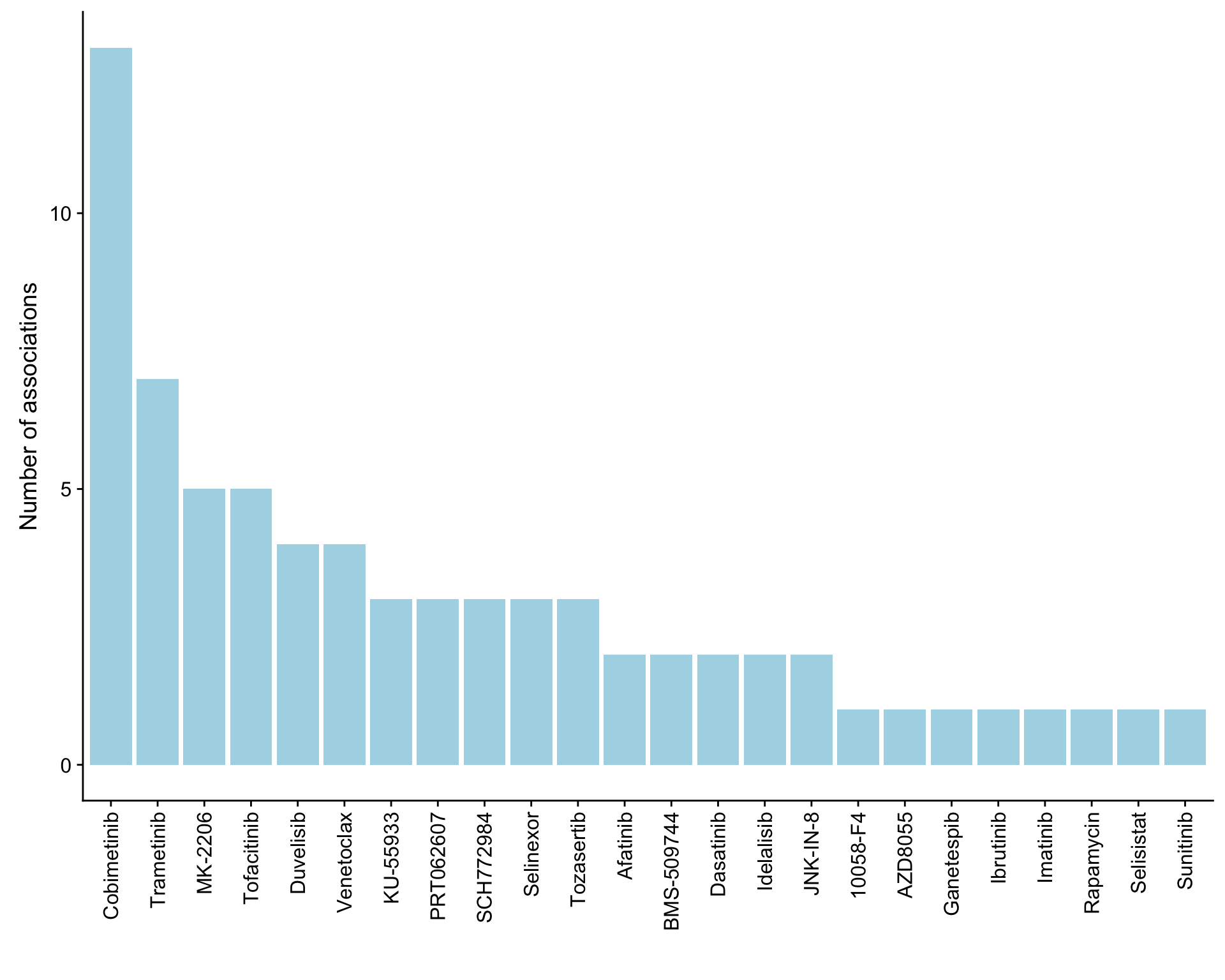
Table of significant associations (10% FDR)
resTab.sig %>% mutate_if(is.numeric, formatC, digits=2, format= "e") %>%
  DT::datatable()
Plot top 9 drug-protein associations
plotList <- lapply(seq(9), function(i) {
  drugConc <- resTab.sig$Drug[i]
  proteinName <- resTab.sig$symbol[i]
  id <- resTab.sig$id[i]
  plotTab <- tibble(patID = colnames(viabMat.auc),
                    viab = viabMat.auc[drugConc,],
                    expr = proMat[id,]) %>%
    mutate(IGHV = protCLL[,patID]$IGHV.status,
           trisomy12 = protCLL[,patID]$trisomy12)
  ggplot(plotTab, aes(x=viab, y=expr)) + geom_point(aes(col = trisomy12, shape = IGHV)) +
    scale_shape_manual(values = c(M = 19, U = 1)) + geom_smooth(method = "lm", se=FALSE) +
    ggtitle(sprintf("%s ~ %s", drugConc, proteinName)) +
    ylab("Protein expression") + xlab("Viability after treatment") +
    theme(legend.position = "bottom")
})
plot_grid(plotlist = plotList, ncol =3)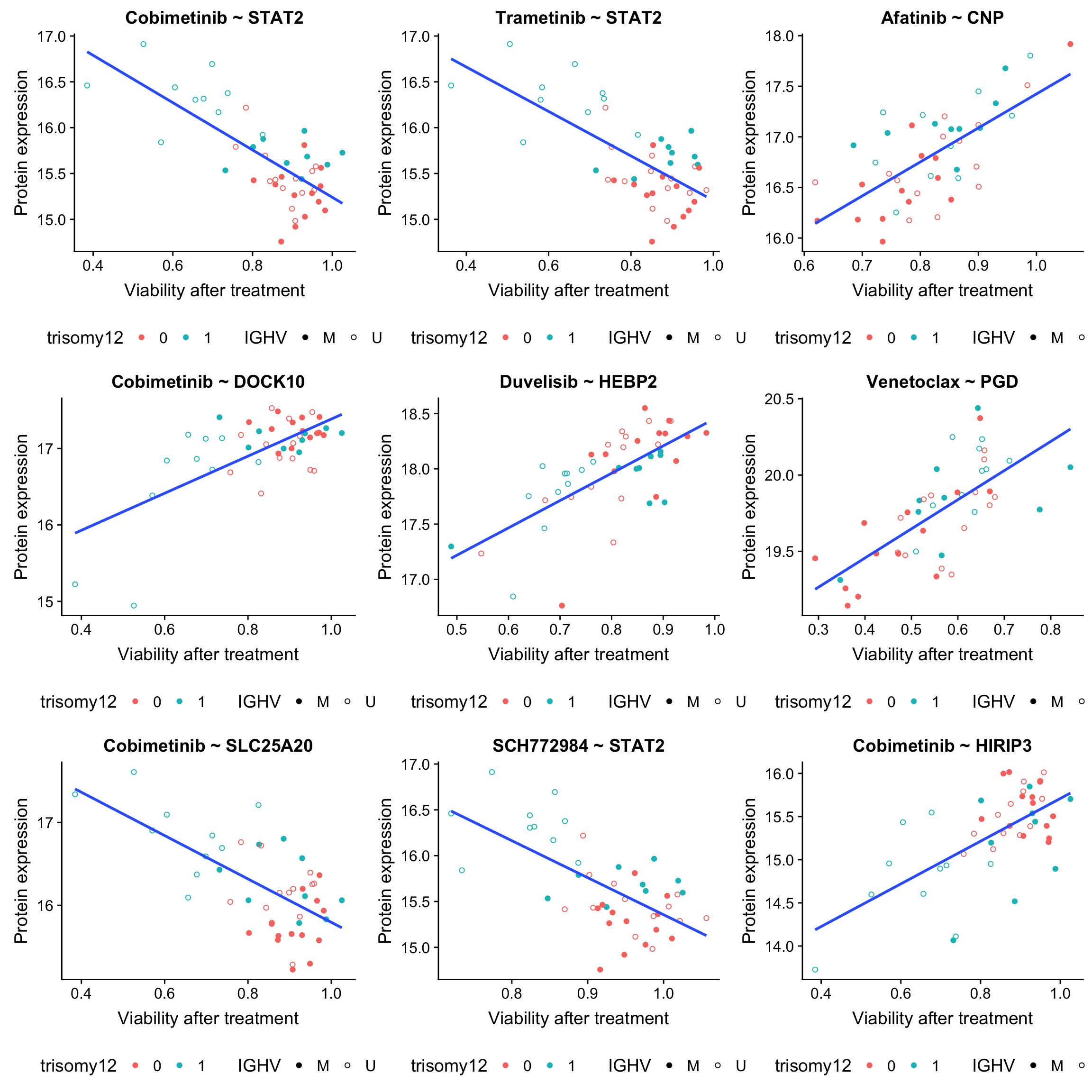
Association test with blocking for IGHV and trisomy12
As IGHV and trisomy12 are associated with both protein abundance and drug responses. I will use multi-variate test to block IGHV and trisomy12 to identify drug-protein associations that are independent of IGHV or trisomy12 status.
The test will be restricted to the associations that were detected as significant (10%) in the model without blocking. Otherwise, none of the associations will be significant after FDR correction.
For individual concentrations
Association test
testList <- filter(resTab, adj.P.Val < 0.1)
resTab.block <- lapply(seq(nrow(testList)),function(i) {
  pair <- testList[i,]
  expr <- proMat[pair$id,]
  viab <- viabMat[pair$drugConc, ]
  ighv <- protCLL[,colnames(viabMat)]$IGHV.status
  tri12 <- protCLL[,colnames(viabMat)]$trisomy12
  res <- anova(lm(viab~ighv+tri12+expr))
  data.frame(id = pair$id, P.Value = res["expr",]$`Pr(>F)`, symbol = pair$symbol,
             drugConc = pair$drugConc, Drug = pair$Drug, concIndex = pair$concIndex,
             P.Value.IGHV = res["ighv",]$`Pr(>F)`,P.Value.trisomy12 = res["tri12",]$`Pr(>F)`,
             P.Value.noBlock = pair$P.Value,
             stringsAsFactors = FALSE)

}) %>% bind_rows() %>% mutate(adj.P.Val = p.adjust(P.Value, method = "BH")) %>% arrange(P.Value)
Number of associations (10% FDR)
Select significant associations
resTab.sig <- filter(resTab.block, adj.P.Val < 0.1) %>%
  select(Drug, symbol, id, P.Value, adj.P.Val, P.Value.trisomy12, P.Value.IGHV, concIndex)
plotTab <- resTab.sig %>% group_by(Drug, concIndex) %>%
summarise(n = length(id)) %>% ungroup()
ordTab <- group_by(plotTab, Drug) %>% summarise(total = sum(n)) %>%
arrange(desc(total))
plotTab <- mutate(plotTab, Drug = factor(Drug, levels = ordTab$Drug)) %>%
filter(n>0)
ggplot(plotTab, aes(x=Drug,y=n,fill = concIndex)) + geom_bar(stat = "identity") +
theme(axis.text.x = element_text(angle = 90,hjust=1,vjust=0.5)) +
ylab("Number of associations") + xlab("")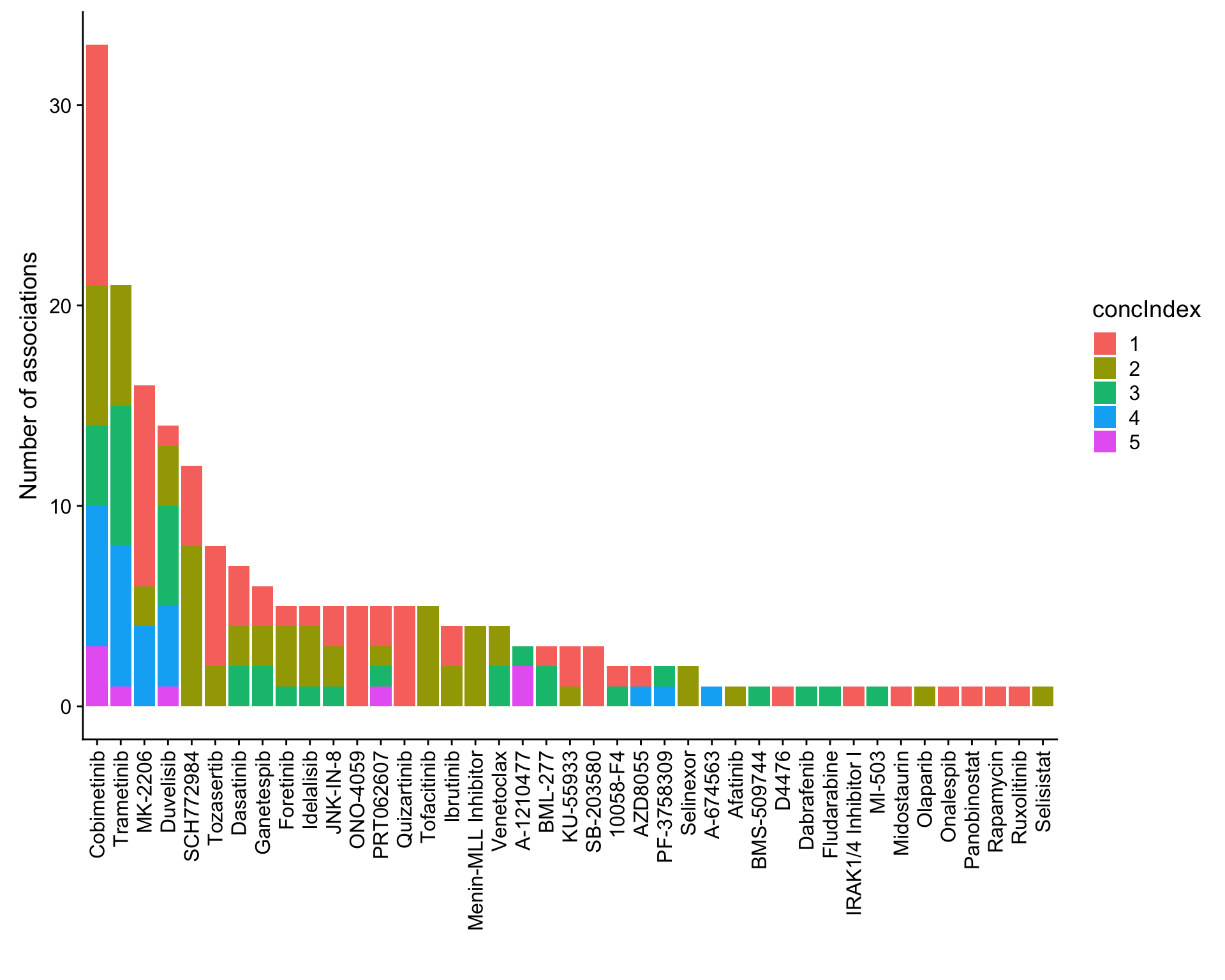
Table of significant associations
resTab.sig %>% mutate_if(is.numeric, formatC, digits=2, format= "e") %>%
DT::datatable()The P.Value.trisomy12 and P.Value.IGHV indicates the drug responses that can be explained by trisomy12 and IGHV, respectively. If the P.Value is highly significant but P.Value.trisomy12 and P.Value.IGHV are not significant (for example, Afatinib-CNP in this table), it means the drug responses can only be explained by protein expression but not IGHV or trisomy12.
Many associations related to MEK/ERK, e.g. Combimetinib-STAT2, have reduced significance here, which is not uprising as trisomy12 is a confounder. But the associations are still significant when blocking for trisomy12 and IGHV, indicating protein expressions can still add information to trisomy12 and IGHV.
Plot top 9 drug-protein associations
plotList <- lapply(seq(9), function(i) {
  drugConc <- paste0(resTab.sig$Drug[i],"_",resTab.sig$concIndex[i])
  proteinName <- resTab.sig$symbol[i]
  id <- resTab.sig$id[i]
  plotTab <- tibble(patID = colnames(viabMat),
                    viab = viabMat[drugConc,],
                    expr = proMat[id,]) %>%
    mutate(IGHV = protCLL[,patID]$IGHV.status,
           trisomy12 = protCLL[,patID]$trisomy12)
  ggplot(plotTab, aes(x=viab, y=expr,col = trisomy12, shape = IGHV, linetype = IGHV)) + geom_point() +
    scale_shape_manual(values = c(M = 19, U = 1)) + geom_smooth(method = "lm", se=FALSE) +
    ggtitle(sprintf("%s ~ %s", drugConc, proteinName)) +
    ylab("Protein expression") + xlab("Viability after treatment") +
    theme(legend.position = "bottom")
})
plot_grid(plotlist = plotList, ncol =3)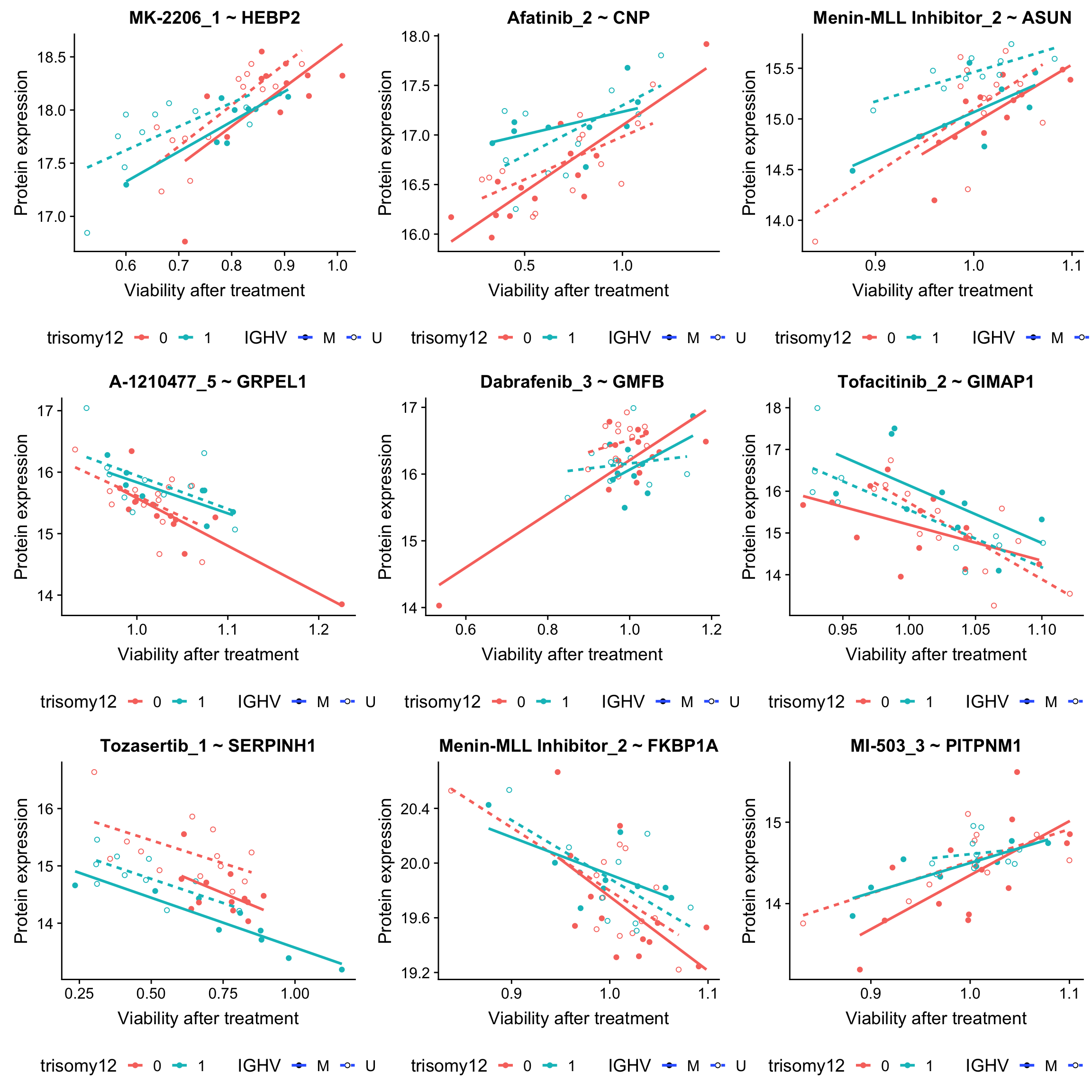
For averaged five concentrations (AUC)
Association test
testList <- filter(resTab.auc, adj.P.Val < 0.1)
resTab.auc.block <- lapply(seq(nrow(testList)),function(i) {
  pair <- testList[i,]
  expr <- proMat[pair$id,]
  viab <- viabMat.auc[pair$Drug, ]
  ighv <- protCLL[,colnames(viabMat.auc)]$IGHV.status
  tri12 <- protCLL[,colnames(viabMat.auc)]$trisomy12
  res <- anova(lm(viab~ighv+tri12+expr))
  data.frame(id = pair$id, P.Value = res["expr",]$`Pr(>F)`, symbol = pair$symbol,
             Drug = pair$Drug,
             P.Value.IGHV = res["ighv",]$`Pr(>F)`,P.Value.trisomy12 = res["tri12",]$`Pr(>F)`,
             P.Value.noBlock = pair$P.Value,
             stringsAsFactors = FALSE)

}) %>% bind_rows() %>% mutate(adj.P.Val = p.adjust(P.Value, method = "BH")) %>% arrange(P.Value)
Number of associations (10% FDR)
Select significant associations
resTab.sig <- filter(resTab.auc.block, adj.P.Val < 0.1) %>%
  select(Drug, symbol, id, P.Value, adj.P.Val, P.Value.trisomy12, P.Value.IGHV)
plotTab <- resTab.sig %>% group_by(Drug) %>%
summarise(n = length(id)) %>% ungroup()
ordTab <- group_by(plotTab, Drug) %>% summarise(total = sum(n)) %>%
arrange(desc(total))
plotTab <- mutate(plotTab, Drug = factor(Drug, levels = ordTab$Drug)) %>%
filter(n>0)
ggplot(plotTab, aes(x=Drug,y=n)) + geom_bar(stat = "identity", fill = "lightblue") +
theme(axis.text.x = element_text(angle = 90,hjust=1,vjust=0.5)) +
ylab("Number of associations") + xlab("")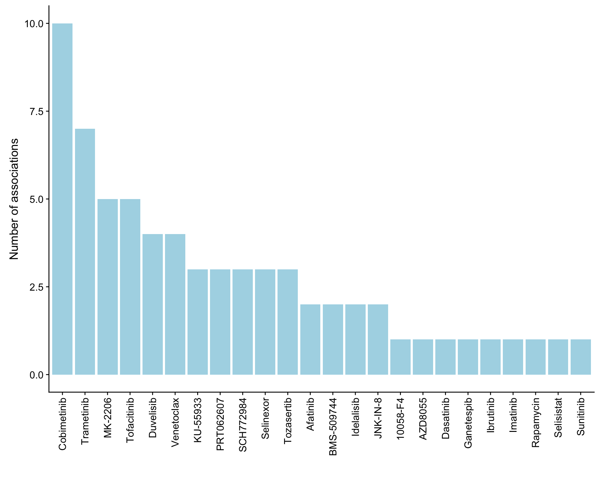
Table of significant associations (10% FDR)
resTab.sig %>% mutate_if(is.numeric, formatC, digits=2, format= "e") %>%
  DT::datatable()
Plot top 9 drug-protein associations
plotList <- lapply(seq(9), function(i) {
  drugConc <- resTab.sig$Drug[i]
  proteinName <- resTab.sig$symbol[i]
  id <- resTab.sig$id[i]
  plotTab <- tibble(patID = colnames(viabMat.auc),
                    viab = viabMat.auc[drugConc,],
                    expr = proMat[id,]) %>%
    mutate(IGHV = protCLL[,patID]$IGHV.status,
           trisomy12 = protCLL[,patID]$trisomy12)
  ggplot(plotTab, aes(x=viab, y=expr,col = trisomy12, shape = IGHV, linetype = IGHV)) + geom_point(aes()) +
    scale_shape_manual(values = c(M = 19, U = 1)) + geom_smooth(method = "lm", se=FALSE) +
    ggtitle(sprintf("%s ~ %s", drugConc, proteinName)) +
    ylab("Protein expression") + xlab("Viability after treatment") +
    theme(legend.position = "bottom")
})
plot_grid(plotlist = plotList, ncol =3)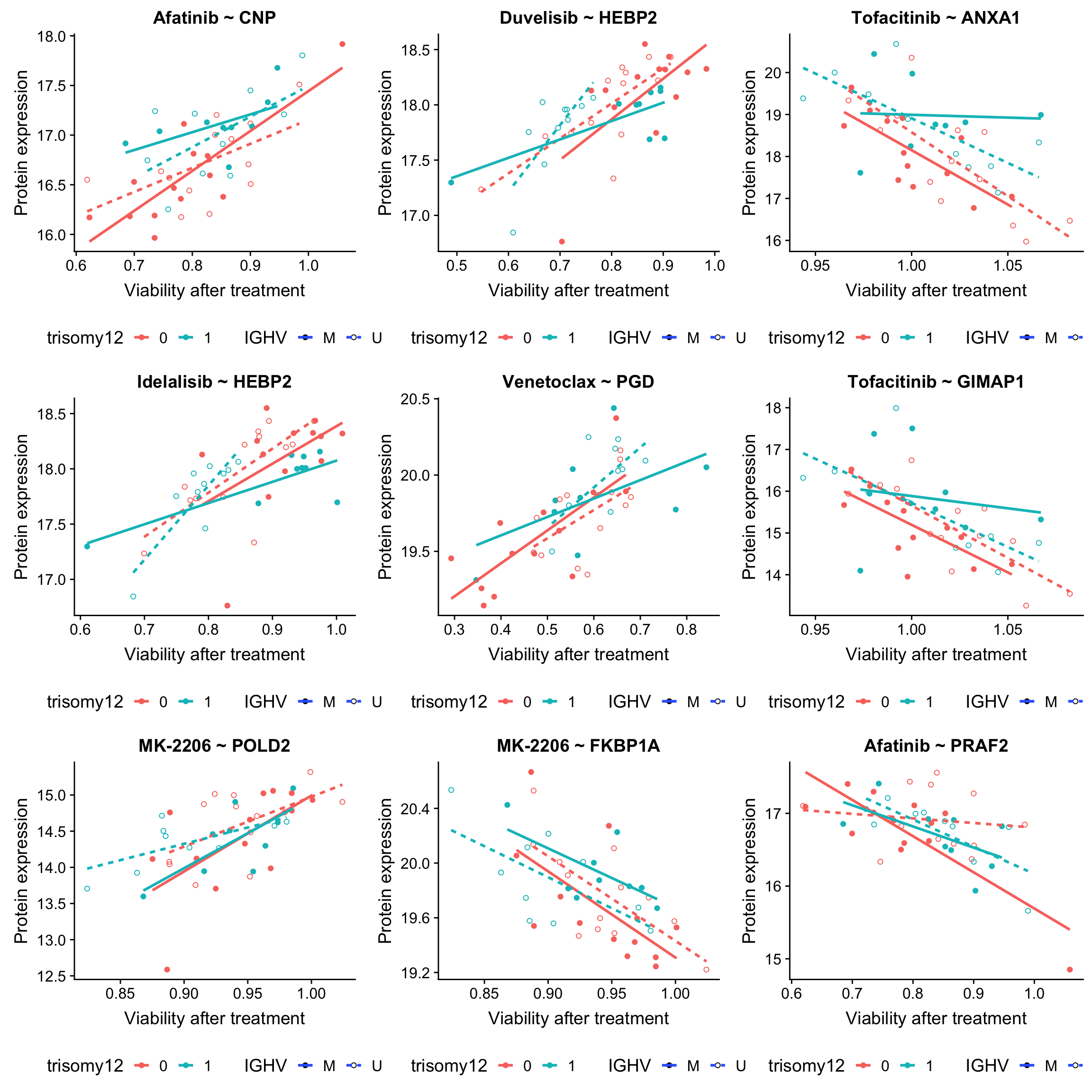
Plot selected drug-protein pairs
Correlation plot
drugList <- list(c("Cobimetinib","STAT2"), c("Venetoclax","PGD"),c("Idelalisib","HEBP2"))
plotList <- lapply(drugList, function(p) {
  drugConc <- p[1]
  proteinName <- p[2]
  id <- unique(filter(resTab.sig, symbol == proteinName)$id)
  plotTab <- tibble(patID = colnames(viabMat.auc),
                    viab = viabMat.auc[drugConc,],
                    expr = proMat[id,]) %>%
    mutate(IGHV = protCLL[,patID]$IGHV.status,
           trisomy12 = protCLL[,patID]$trisomy12)
  ggplot(plotTab, aes(x=viab, y=expr)) + geom_point(aes(col = trisomy12, shape = IGHV)) +
    scale_shape_manual(values = c(M = 19, U = 1)) + geom_smooth(method = "lm", se=FALSE) +
    ggtitle(sprintf("%s ~ %s", drugConc, proteinName)) +
    ylab("Protein expression") + xlab("Viability after treatment") +
    theme(legend.position = "bottom")
})
plot_grid(plotlist = plotList, ncol =1)
Variance explained
Test whether the protein expression can explain additional variance in drug response compared to genetic alone
Prepare genomics
geneMat <-  patMeta[match(colnames(proMat), patMeta$Patient.ID),] %>%
  select(Patient.ID, IGHV.status, del11p:U1) %>%
  mutate_if(is.factor, as.character) %>% mutate(IGHV.status = ifelse(IGHV.status == "M", 1,0)) %>%
  mutate_at(vars(-Patient.ID), as.numeric) %>% #assign a few unknown mutated cases to wildtype
  mutate_all(replace_na,0) %>%
  data.frame() %>% column_to_rownames("Patient.ID")


geneMat <- geneMat[,apply(geneMat,2, function(x) sum(x %in% 1, na.rm = TRUE))>=5] %>% as.matrix()
Genes that will be included in the multivariate model
colnames(geneMat)[1] "IGHV.status" "del11q" "del13q" "trisomy12" "DDX3X"
[6] "EGR2" "NOTCH1" "SF3B1" "TP53" compareR2 <- function(Drug, protName, geneMat) {
viab <- viabMat.auc[Drug,]
protID <- unique(filter(resTab.sig, symbol == protName)$id)
expr <- proMat[protID,]
tabGene <- data.frame(geneMat)
tabGene[["viab"]] <- viab
tabCom <- tabGene
tabCom[[protName]] <- expr
r2Prot <- summary(lm(viab~expr))$r.squared
r2Gene <- summary(lm(viab~., data=tabGene))$r.squared
r2Com <- summary(lm(viab~., data=tabCom))$r.squared
plotTab <- tibble(model = c("genetics",paste0(protName, " expression"),sprintf("genetics + %s expression",protName)),
R2 = c(r2Gene, r2Prot, r2Com))
ggplot(plotTab, aes(x=model, y = R2)) + geom_bar(aes(fill = model),stat="identity") + coord_flip() +
theme(legend.position = "none") + ggtitle(Drug) + xlab("Variance expalained (R2)")
}plotList <- lapply(drugList, function(p) {
compareR2(p[1],p[2],geneMat)
})
plot_grid(plotlist= plotList, ncol= 1) Based on the plot of R2 values, including protein expression in multi-variate model could explain additional variance in drug responses compared to genetic alone. For Venetoclax, using a single protein expression value of PGD already explain more variance than genetics.
Compare the ability to explain drug response among genomic, RNA and protein data
Prepare data
Proteomics data
proMat <- assays(protCLL)[["QRILC"]]
proMat <- proMat[,colnames(viabMat.auc)]
sds <- genefilter::rowSds(proMat,na.rm=TRUE)
proMat <- proMat[sds > genefilter::shorth(sds),]
removeCorrelated <- function(x, cutoff = 0.8, distance = "cosine", cluster_method = "ward.D2") {
# calculate distiance matrix
if (distance == "binary") {
#maybe also usefull is the input is a sparse matrix
distMat <- dist(t(x), method = "binary")
} else if (distance == "pearson") {
#otherwise, using pearson correlation
distMat <- as.dist(1-cor(x))
} else if (distance == "euclidean") {
distMat <- dist(t(x), method = "euclidean")
} else if (distance == "cosine") {
# cosine similarity maybe prefered for sparse matrix
cosineSimi <- function(x){
x%*%t(x)/(sqrt(rowSums(x^2) %*% t(rowSums(x^2))))
}
distMat <- as.dist(1-cosineSimi(t(x)))
} else if (distance == "canberra") {
distMat <- as.dist(as.matrix(dist(t(x), method = "canberra"))/nrow(x))
}
#hierarchical clustering
hc <- hclust(distMat, method = cluster_method)
clusters <- cutree(hc, h = 1-cutoff)
x.re <- x[,!duplicated(clusters)]
#record the removed features
mapList <- lapply(colnames(x.re), function(i) {
members <- names(clusters[clusters == clusters[i]])
members[members != i]
})
names(mapList) <- colnames(x.re)
return(list(reduced = x.re,
mapReduce = mapList))
}Remove highly correlated proteins
proReduced <- removeCorrelated(t(proMat), cutoff = 0.9, distance = "pearson")
proMat.re <- t(proReduced$reduced)
Subset samples
overSample <- intersect(colnames(proMat.re), colnames(dds))
proMat.glm <- proMat.re[,overSample]
viabMat.glm <- viabMat.auc[,overSample]
dds.glm <- dds[,overSample]
Prepare expression data
ddsSub.glm <- dds.glm[rowSums(counts(dds.glm)) > 100,]
ddsSub.glm <- varianceStabilizingTransformation(ddsSub.glm)
exprMat <- assay(ddsSub.glm)
sds <- genefilter::rowSds(exprMat)
exprMat <- exprMat[order(sds, decreasing=T)[1:5000],]

reduceRes <- removeCorrelated(t(exprMat), cutoff = 0.9, distance = "pearson")
exprMat.glm <- t(reduceRes$reduced)
Prepare genomic data
geneMat <-  patMeta[match(overSample, patMeta$Patient.ID),] %>%
  select(Patient.ID, IGHV.status, del11p:U1) %>%
  mutate_if(is.factor, as.character) %>% mutate(IGHV.status = ifelse(IGHV.status == "M", 1,0)) %>%
  mutate_at(vars(-Patient.ID), as.numeric) %>% #assign a few unknown mutated cases to wildtype
  data.frame() %>% column_to_rownames("Patient.ID")


geneMat <- geneMat[,apply(geneMat,2, function(x) sum(x %in% 1, na.rm = TRUE))>=3]
geneMat[is.na(geneMat)] <- 0
Feature selection using LASSO
Prepare clean data: Integrate all available multi-omics datasets.
inclSet<-list(RNA=t(proMat.glm), drugs= t(viabMat.glm), Protein = t(proMat.glm), gen = geneMat)
cleanData <- generateData(inclSet, censor = 5)
Perform lasso regression (3-fold repeated CV)
lassoResults <- list()
for (eachMeasure in names(cleanData$allResponse)) {
  dataResult <- list()
  for (eachDataset in names(cleanData$allExplain)) {
    y <- cleanData$allResponse[[eachMeasure]]
    X <- cleanData$allExplain[[eachDataset]]


    glmRes <- runGlm(X, y, method = "lasso", repeats = 20, folds = 3)
    dataResult[[eachDataset]] <- glmRes
  }
  lassoResults[[eachMeasure]] <- dataResult
}
save(lassoResults, file = "../output/lassoResults_CPS.RData", version = 2)
Visualizing results
load("../output/lassoResults_CPS.RData")Variane explained (R2)
Averaged R2 for all drugs
#load save data
outList.train <- plotVar(lassoResults,cv=FALSE)
outList.cv <- plotVar(lassoResults, cv=TRUE)


sumTab.cv <- outList.cv$summary %>% mutate(group = "CV")
sumTab.train <- outList.train$summary %>% mutate(group = "train")
sumTab <- bind_rows(sumTab.train, sumTab.cv)

std <- function(x) sd(x)/sqrt(length(x))

plotTab <- sumTab %>%
  group_by(set,group) %>% summarise(R2 = mean(meanR2), sem = std(meanR2))
ggplot(plotTab, aes(x=set, y = R2, fill = group)) + geom_bar(stat="identity", width = 0.5, position = "dodge") +
  geom_errorbar(aes(ymin = R2 -sem, ymax=R2+sem), width= 0.5, position = "dodge") +
  theme(legend.position = "none") + theme_bw()
It can be seen that the R2 for cross-validating (CV) set is generally much lower than training set. This is a sign of significant over-fitting, which is not unexpected due to we have many features but very few samples. So perhaps regularised multi-variate analysis is not very suitable here.
For individual drugs
plotTab <- filter(sumTab, set != "")
#rank by variance explained by proteomics data
drugRank <- plotTab %>% filter(set == "protein", group == "CV") %>% arrange(desc(meanR2)) %>% pull(drug)

plotList <- lapply(drugRank, function(name){
  eachTab <- filter(plotTab, drug == name)

  ggplot(eachTab,(aes(x=set, y = meanR2, fill = group))) +
    geom_bar(stat ="identity",position = "dodge2", width=0.5) +
    ggtitle(name) + coord_cartesian(ylim = c(0,1)) +
    geom_errorbar(aes(ymax = meanR2 + sdR2, ymin = meanR2-sdR2), position = "dodge2", width=0.5) +
    theme_bw() + theme(legend.position = "none")
})

plot_grid(plotlist = plotList, ncol =3)
Proteins selected for each drug
Here I only use the top 10 drugs that best explained by proteomics
drugList <- drugRank[1:10]
plotList <- lapply(drugList,function(n) {
  plotMat <- lassoResults[[n]]$protein$coefMat
  plotMat <- plotMat[rowMeans(plotMat)!=0,]
  plotTab <- plotMat %>% data.frame() %>% rownames_to_column("id") %>%
    gather(key = "rep",value = "coef",-id) %>%
    group_by(id) %>% summarise(meanCoef = mean(coef),semCoef=std(coef),freq=mean(sign(abs(coef)))) %>%
    mutate(id=str_remove(id,"con.protein")) %>%
    mutate(symbol = rowData(protCLL[id,])$hgnc_symbol) %>%
    arrange(desc(meanCoef)) %>% mutate(symbol = factor(symbol, levels = symbol))
  ggplot(plotTab, aes(x=symbol,y=meanCoef,fill = freq)) +
    geom_bar(stat = "identity") + geom_errorbar(aes(ymax=meanCoef+semCoef, ymin = meanCoef-semCoef)) +
    scale_fill_gradient(high="darkred", low="darkblue",name ="frequency", limits=c(0,1)) +
    theme(legend.position = "right", axis.text.x = element_text(angle = 90, hjust=1, vjust = 0.5)) +
    ggtitle(n) +
    ylab("Coefficient") + xlab("")

})

plotList
[[1]]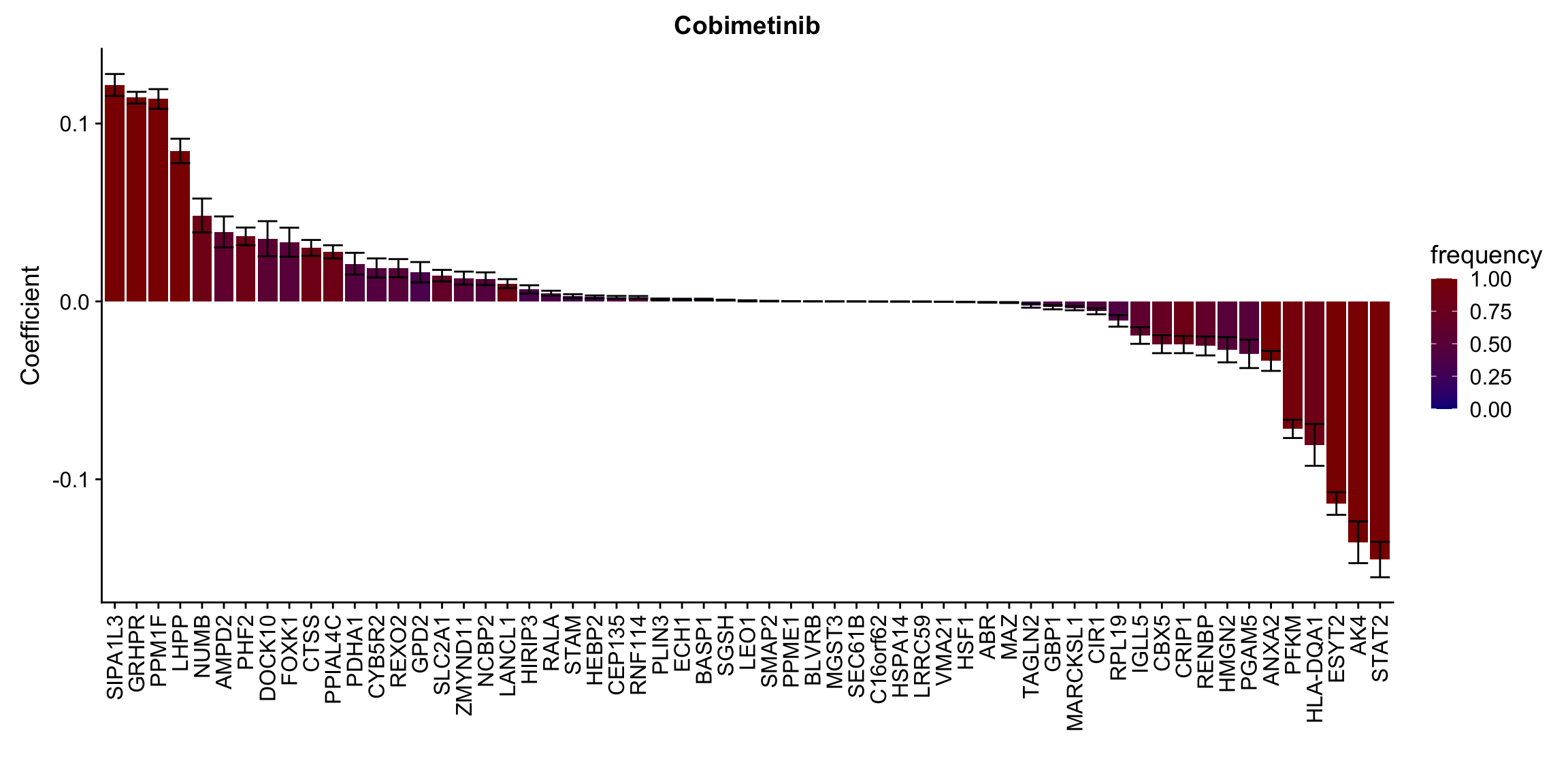
[[2]]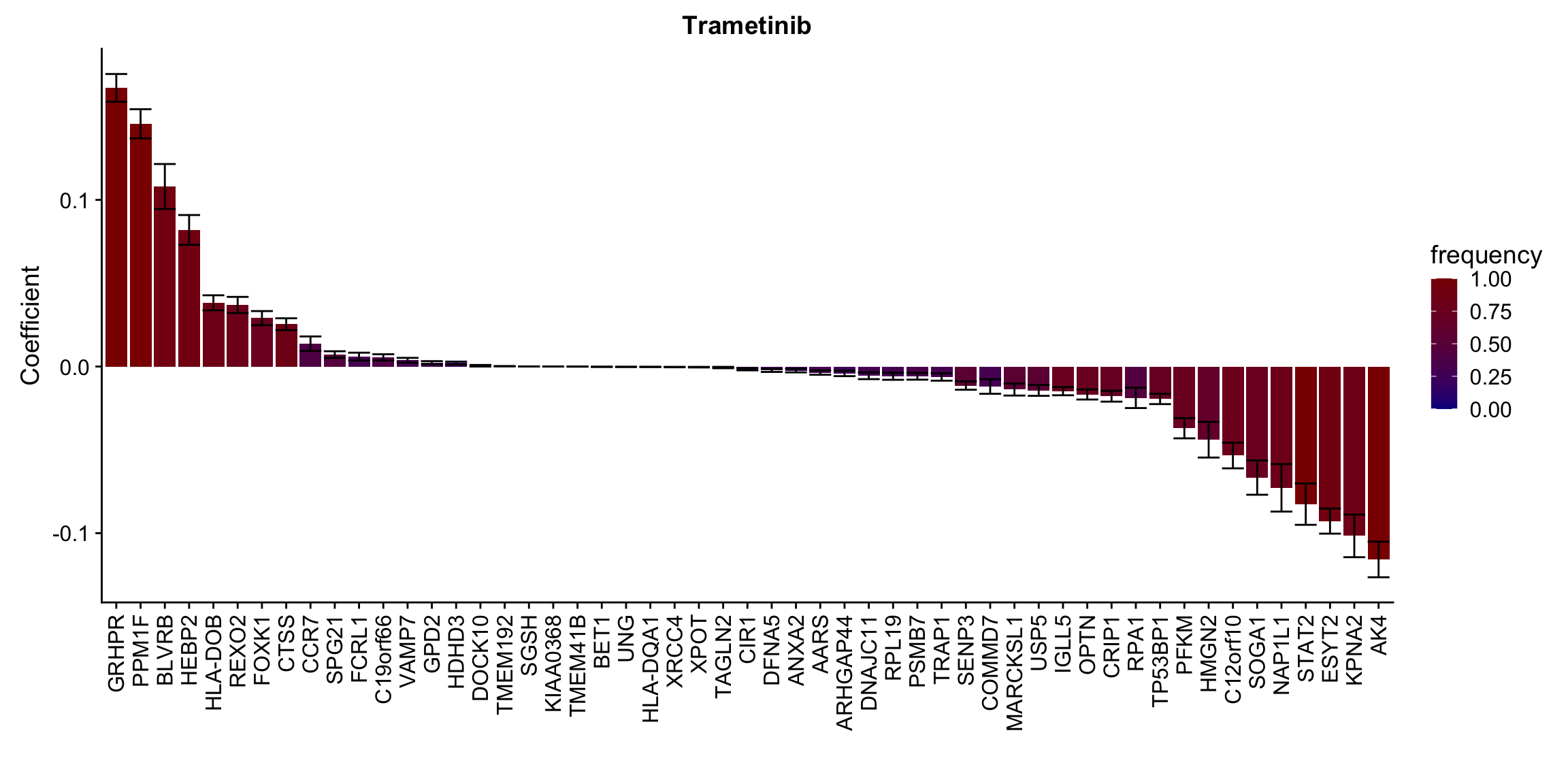
[[3]]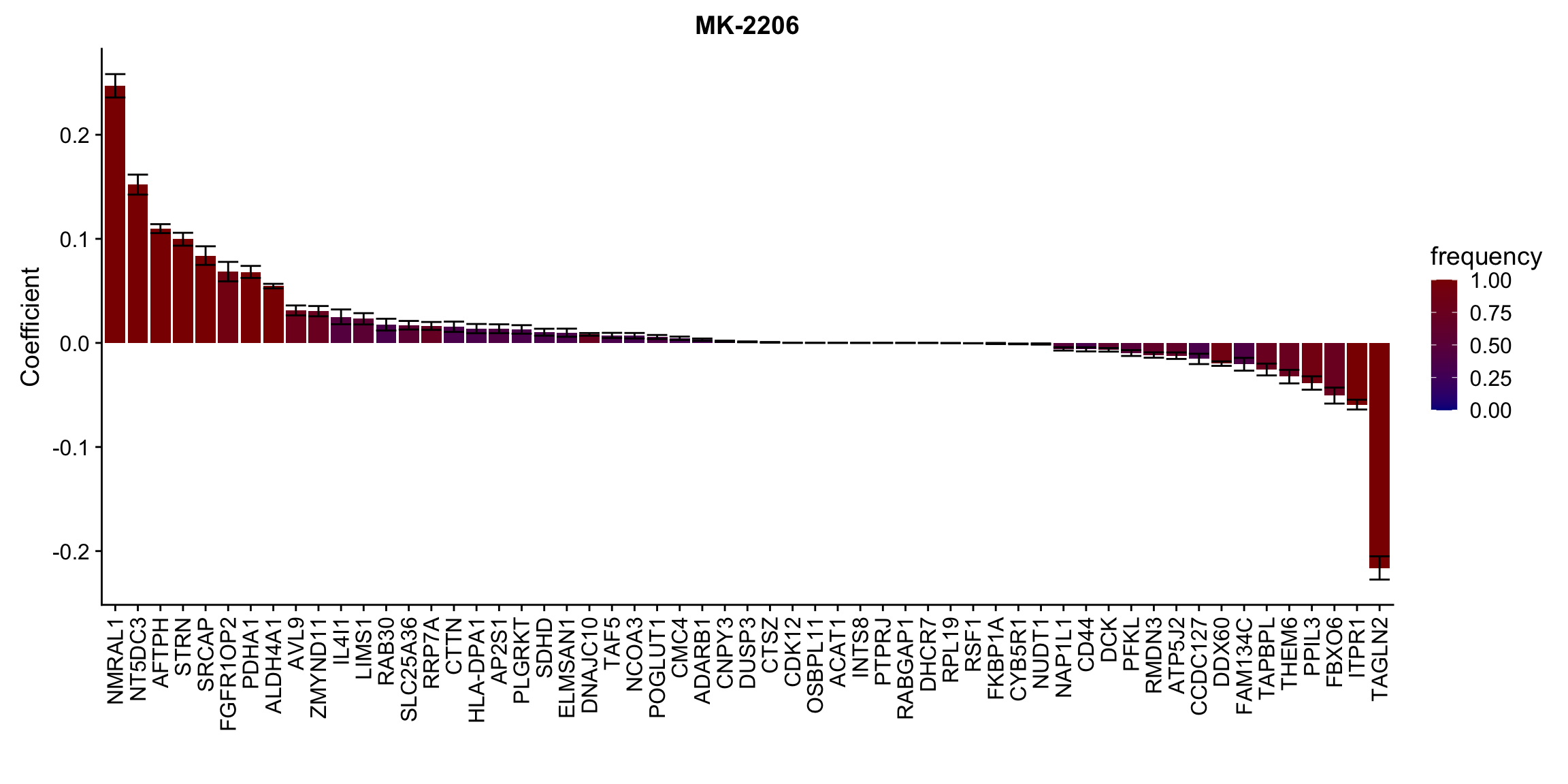
[[4]]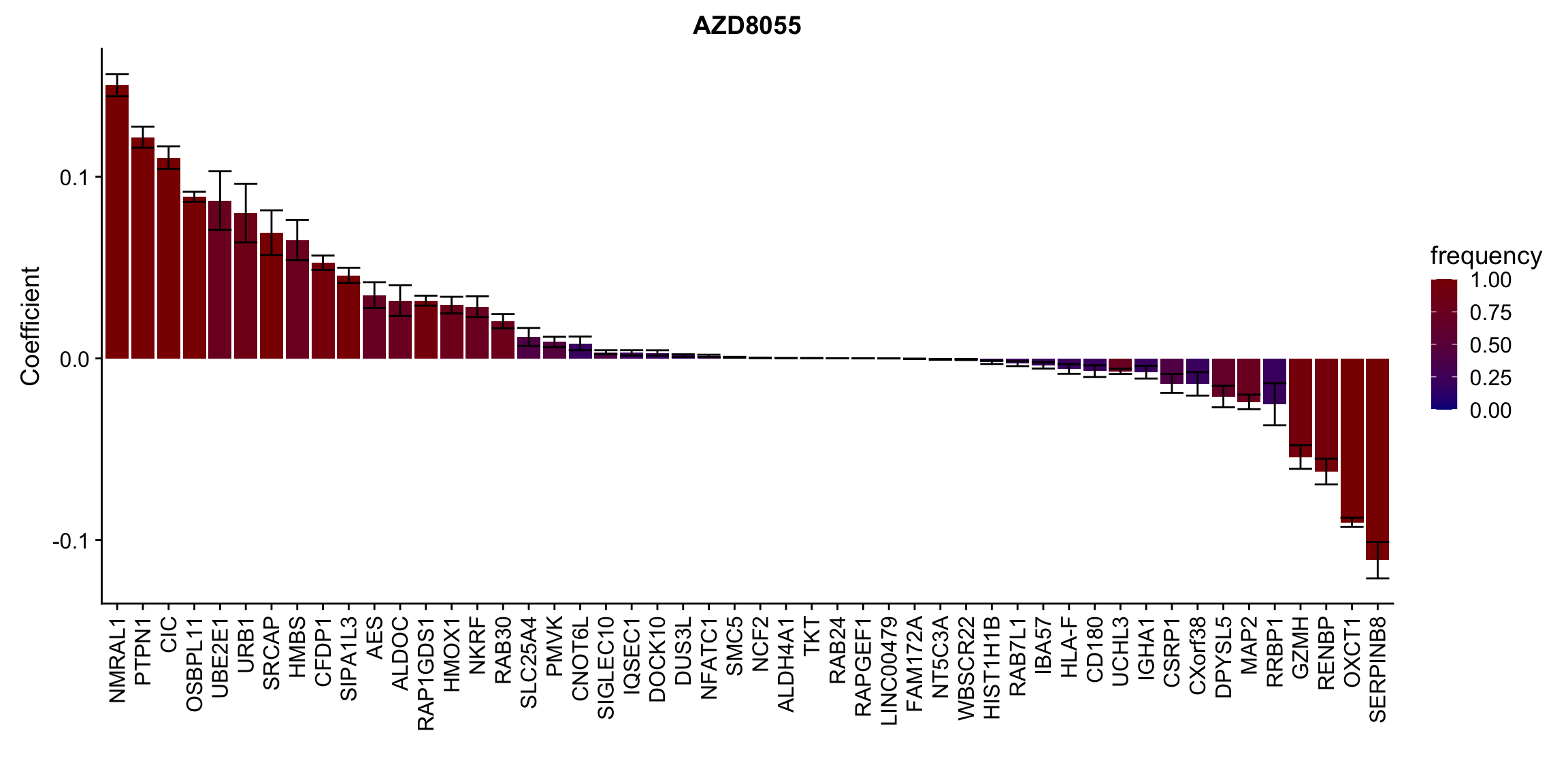
[[5]]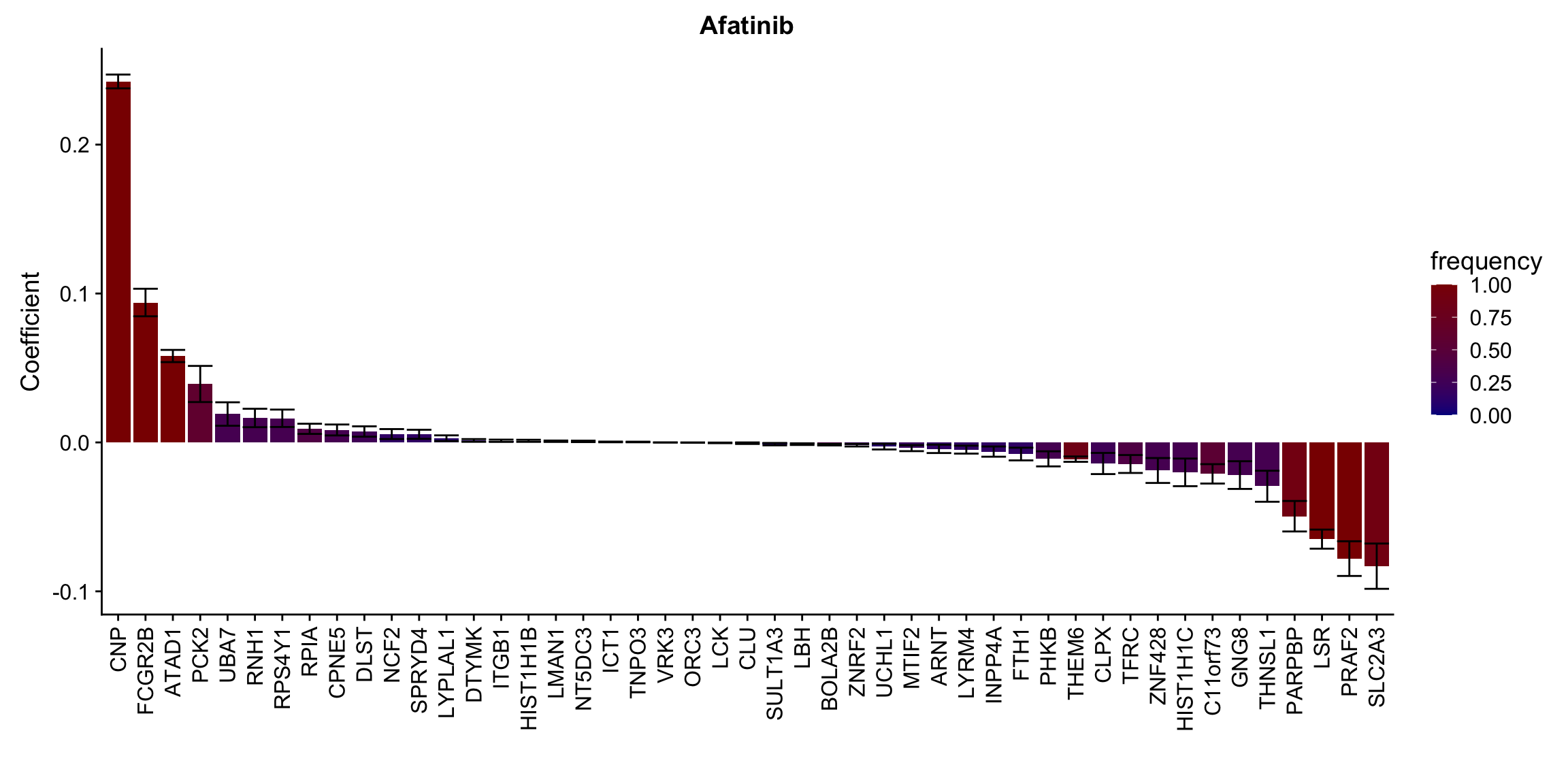
[[6]]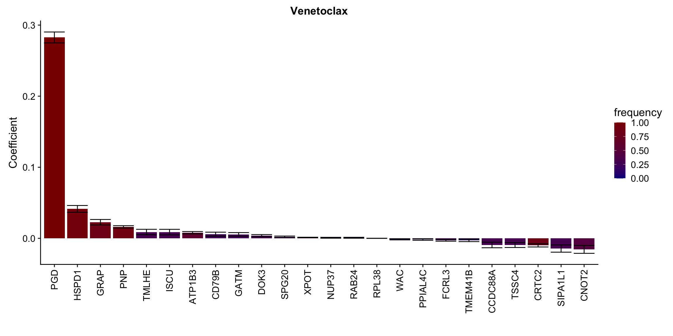
[[7]]
[[8]]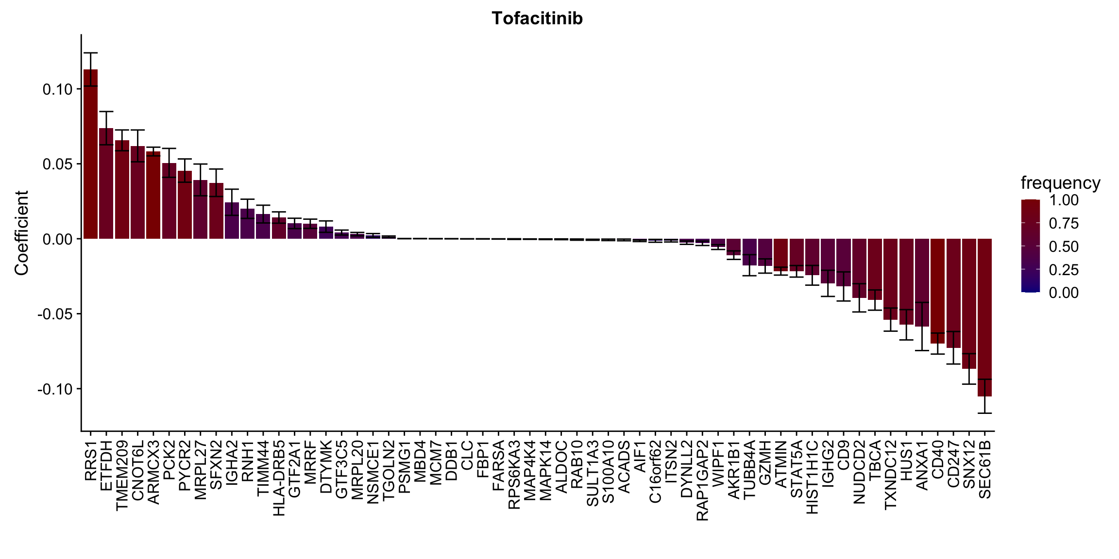
[[9]]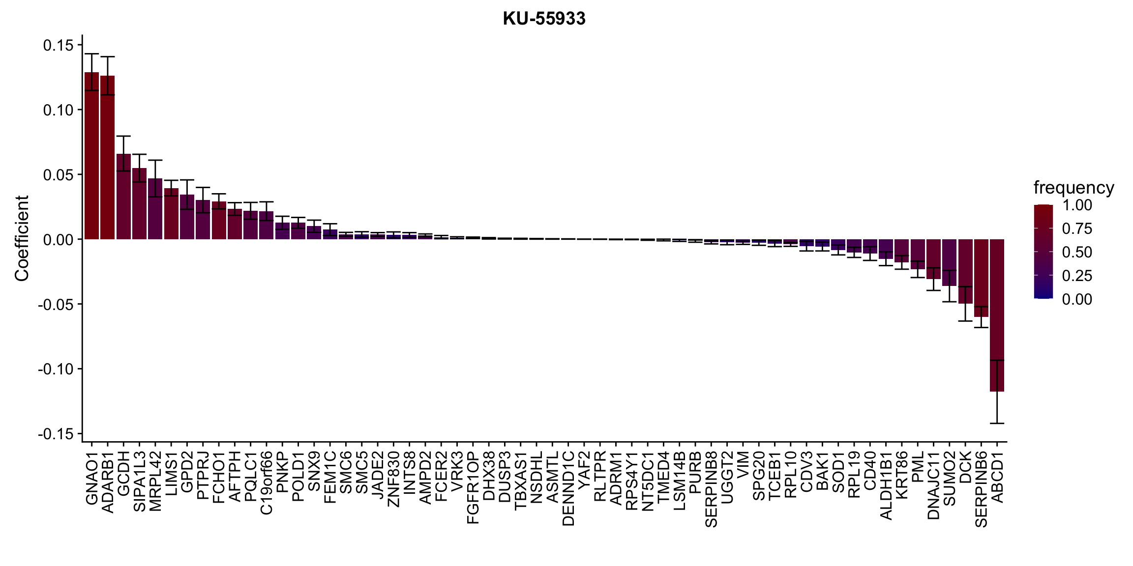
[[10]]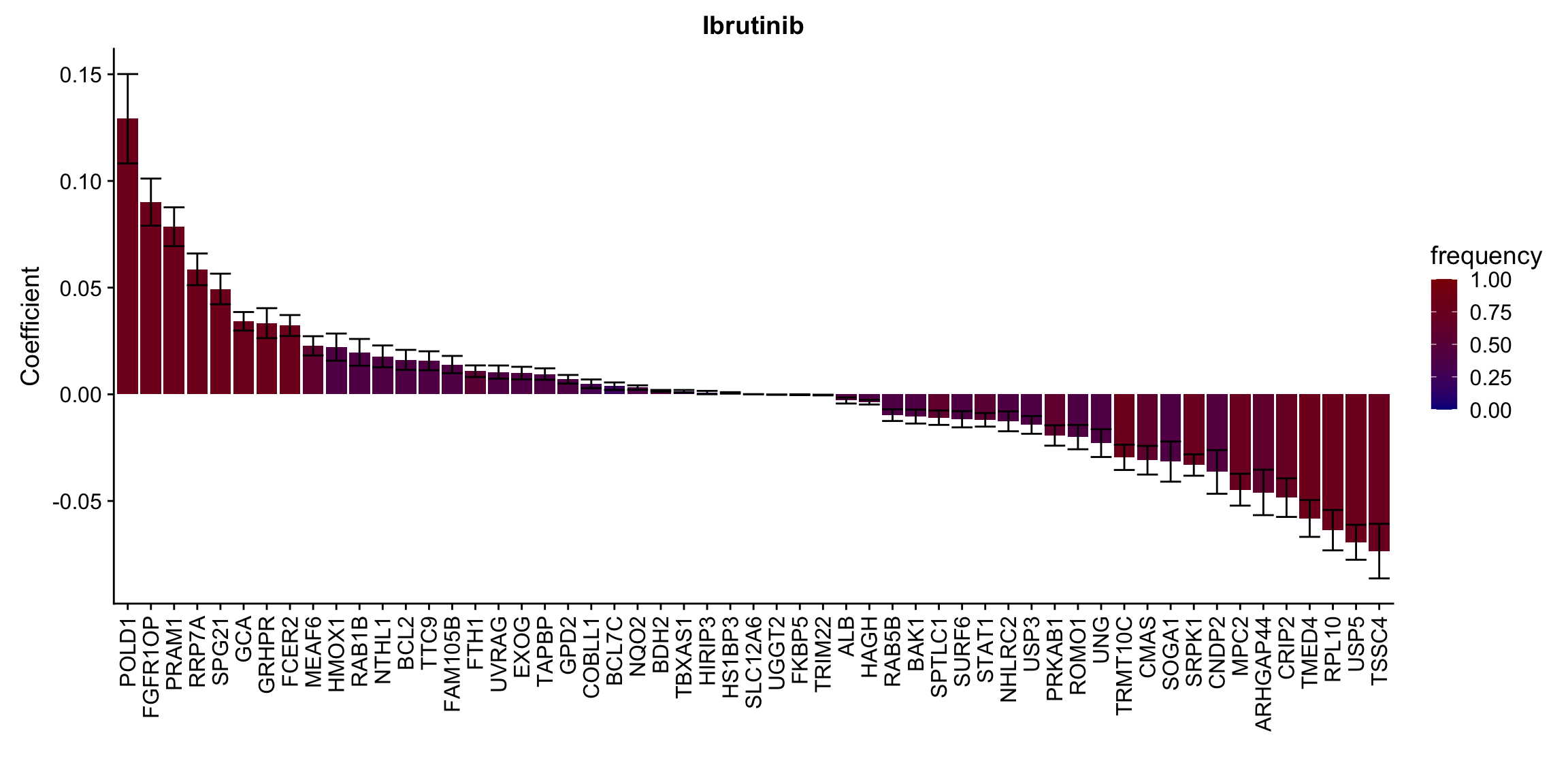 In general, if the proteins show high correlation with drug response in uni-variate test, they will be selected here.
Also note that there are more features selected than sample size (N >p), which is also a sign of over-fitting.
sessionInfo()R version 3.6.0 (2019-04-26)
Platform: x86_64-apple-darwin15.6.0 (64-bit)
Running under: macOS 10.15.4
Matrix products: default
BLAS: /Library/Frameworks/R.framework/Versions/3.6/Resources/lib/libRblas.0.dylib
LAPACK: /Library/Frameworks/R.framework/Versions/3.6/Resources/lib/libRlapack.dylib
locale:
[1] en_US.UTF-8/en_US.UTF-8/en_US.UTF-8/C/en_US.UTF-8/en_US.UTF-8
attached base packages:
[1] parallel stats4 stats graphics grDevices utils datasets
[8] methods base
other attached packages:
[1] DESeq2_1.24.0 forcats_0.4.0
[3] stringr_1.4.0 dplyr_0.8.5
[5] purrr_0.3.3 readr_1.3.1
[7] tidyr_1.0.0 tibble_3.0.0
[9] tidyverse_1.3.0 SummarizedExperiment_1.14.0
[11] DelayedArray_0.10.0 BiocParallel_1.18.0
[13] matrixStats_0.54.0 Biobase_2.44.0
[15] GenomicRanges_1.36.0 GenomeInfoDb_1.20.0
[17] IRanges_2.18.1 S4Vectors_0.22.0
[19] BiocGenerics_0.30.0 glmnet_2.0-18
[21] foreach_1.4.4 Matrix_1.2-17
[23] jyluMisc_0.1.5 pheatmap_1.0.12
[25] cowplot_0.9.4 ggplot2_3.3.0
[27] limma_3.40.2
loaded via a namespace (and not attached):
[1] shinydashboard_0.7.1 tidyselect_1.0.0 RSQLite_2.1.1
[4] AnnotationDbi_1.46.0 htmlwidgets_1.3 grid_3.6.0
[7] maxstat_0.7-25 munsell_0.5.0 codetools_0.2-16
[10] DT_0.7 withr_2.1.2 colorspace_1.4-1
[13] knitr_1.23 rstudioapi_0.10 ggsignif_0.5.0
[16] labeling_0.3 git2r_0.26.1 slam_0.1-45
[19] GenomeInfoDbData_1.2.1 KMsurv_0.1-5 bit64_0.9-7
[22] farver_2.0.3 rprojroot_1.3-2 vctrs_0.2.4
[25] generics_0.0.2 TH.data_1.0-10 xfun_0.8
[28] sets_1.0-18 R6_2.4.0 locfit_1.5-9.1
[31] bitops_1.0-6 fgsea_1.10.0 assertthat_0.2.1
[34] promises_1.0.1 scales_1.1.0 multcomp_1.4-10
[37] nnet_7.3-12 gtable_0.3.0 sandwich_2.5-1
[40] workflowr_1.6.0 rlang_0.4.5 genefilter_1.66.0
[43] cmprsk_2.2-8 splines_3.6.0 acepack_1.4.1
[46] broom_0.5.2 checkmate_2.0.0 yaml_2.2.0
[49] abind_1.4-5 modelr_0.1.5 crosstalk_1.0.0
[52] backports_1.1.4 httpuv_1.5.1 Hmisc_4.2-0
[55] tools_3.6.0 relations_0.6-8 ellipsis_0.2.0
[58] gplots_3.0.1.1 RColorBrewer_1.1-2 Rcpp_1.0.1
[61] base64enc_0.1-3 visNetwork_2.0.7 zlibbioc_1.30.0
[64] RCurl_1.95-4.12 ggpubr_0.2.1 rpart_4.1-15
[67] zoo_1.8-6 haven_2.2.0 cluster_2.1.0
[70] exactRankTests_0.8-30 fs_1.4.0 magrittr_1.5
[73] data.table_1.12.2 openxlsx_4.1.0.1 reprex_0.3.0
[76] survminer_0.4.4 mvtnorm_1.0-11 hms_0.5.2
[79] shinyjs_1.0 mime_0.7 evaluate_0.14
[82] xtable_1.8-4 XML_3.98-1.20 rio_0.5.16
[85] readxl_1.3.1 gridExtra_2.3 compiler_3.6.0
[88] KernSmooth_2.23-15 crayon_1.3.4 htmltools_0.4.0
[91] mgcv_1.8-28 later_0.8.0 Formula_1.2-3
[94] geneplotter_1.62.0 lubridate_1.7.4 DBI_1.0.0
[97] dbplyr_1.4.2 MASS_7.3-51.4 car_3.0-3
[100] cli_1.1.0 marray_1.62.0 gdata_2.18.0
[103] igraph_1.2.4.1 pkgconfig_2.0.2 km.ci_0.5-2
[106] foreign_0.8-71 piano_2.0.2 xml2_1.2.2
[109] annotate_1.62.0 XVector_0.24.0 drc_3.0-1
[112] rvest_0.3.5 digest_0.6.19 rmarkdown_1.13
[115] cellranger_1.1.0 fastmatch_1.1-0 survMisc_0.5.5
[118] htmlTable_1.13.1 curl_3.3 shiny_1.3.2
[121] gtools_3.8.1 lifecycle_0.2.0 nlme_3.1-140
[124] jsonlite_1.6 carData_3.0-2 pillar_1.4.3
[127] lattice_0.20-38 httr_1.4.1 plotrix_3.7-6
[130] survival_2.44-1.1 glue_1.3.2 zip_2.0.2
[133] iterators_1.0.10 bit_1.1-14 stringi_1.4.3
[136] blob_1.1.1 latticeExtra_0.6-28 caTools_1.17.1.2
[139] memoise_1.1.0