Principal components analysis and enrichment analysis on PCs
Junyan Lu
2020-03-13
Last updated: 2020-06-06
Checks: 6 1
Knit directory: Proteomics/analysis/
This reproducible R Markdown analysis was created with workflowr (version 1.6.0). The Checks tab describes the reproducibility checks that were applied when the results were created. The Past versions tab lists the development history.
The R Markdown is untracked by Git. To know which version of the R Markdown file created these results, you’ll want to first commit it to the Git repo. If you’re still working on the analysis, you can ignore this warning. When you’re finished, you can run wflow_publish to commit the R Markdown file and build the HTML.
Great job! The global environment was empty. Objects defined in the global environment can affect the analysis in your R Markdown file in unknown ways. For reproduciblity it’s best to always run the code in an empty environment.
The command set.seed(20200227) was run prior to running the code in the R Markdown file. Setting a seed ensures that any results that rely on randomness, e.g. subsampling or permutations, are reproducible.
Great job! Recording the operating system, R version, and package versions is critical for reproducibility.
Nice! There were no cached chunks for this analysis, so you can be confident that you successfully produced the results during this run.
Great job! Using relative paths to the files within your workflowr project makes it easier to run your code on other machines.
Great! You are using Git for version control. Tracking code development and connecting the code version to the results is critical for reproducibility. The version displayed above was the version of the Git repository at the time these results were generated.
Note that you need to be careful to ensure that all relevant files for the analysis have been committed to Git prior to generating the results (you can use wflow_publish or wflow_git_commit). workflowr only checks the R Markdown file, but you know if there are other scripts or data files that it depends on. Below is the status of the Git repository when the results were generated:
Ignored files:
    Ignored:    .DS_Store
    Ignored:    .Rhistory
    Ignored:    .Rproj.user/
    Ignored:    analysis/.DS_Store
    Ignored:    analysis/.Rhistory
    Ignored:    analysis/complexAnalysis_IGHV_alternative_cache/
    Ignored:    analysis/complexAnalysis_IGHV_cache/
    Ignored:    analysis/complexAnalysis_trisomy12_alteredPQR_cache/
    Ignored:    analysis/complexAnalysis_trisomy12_alternative_cache/
    Ignored:    analysis/complexAnalysis_trisomy12_cache/
    Ignored:    analysis/correlateCLLPD_cache/
    Ignored:    analysis/figure/
    Ignored:    code/.Rhistory
    Ignored:    data/.DS_Store
    Ignored:    output/.DS_Store

Untracked files:
    Untracked:  analysis/CNVanalysis_11q.Rmd
    Untracked:  analysis/CNVanalysis_trisomy12.Rmd
    Untracked:  analysis/CNVanalysis_trisomy19.Rmd
    Untracked:  analysis/analysisPCA.Rmd
    Untracked:  analysis/analysisSplicing.Rmd
    Untracked:  analysis/analysisTrisomy19.Rmd
    Untracked:  analysis/annotateCNV.Rmd
    Untracked:  analysis/complexAnalysis_IGHV.Rmd
    Untracked:  analysis/complexAnalysis_IGHV_alternative.Rmd
    Untracked:  analysis/complexAnalysis_overall.Rmd
    Untracked:  analysis/complexAnalysis_trisomy12.Rmd
    Untracked:  analysis/complexAnalysis_trisomy12_alternative.Rmd
    Untracked:  analysis/correlateGenomic_PC12adjusted.Rmd
    Untracked:  analysis/correlateGenomic_noBlock.Rmd
    Untracked:  analysis/correlateGenomic_noBlock_MCLL.Rmd
    Untracked:  analysis/correlateGenomic_noBlock_UCLL.Rmd
    Untracked:  analysis/default.css
    Untracked:  analysis/del11q.pdf
    Untracked:  analysis/del11q_norm.pdf
    Untracked:  analysis/peptideValidate.Rmd
    Untracked:  analysis/plotExpressionCNV.Rmd
    Untracked:  analysis/processPeptides_LUMOS.Rmd
    Untracked:  analysis/style.css
    Untracked:  analysis/trisomy12.pdf
    Untracked:  analysis/trisomy12_AFcor.Rmd
    Untracked:  analysis/trisomy12_norm.pdf
    Untracked:  code/AlteredPQR.R
    Untracked:  code/utils.R
    Untracked:  data/190909_CLL_prot_abund_med_norm.tsv
    Untracked:  data/190909_CLL_prot_abund_no_norm.tsv
    Untracked:  data/20190423_Proteom_submitted_samples_bereinigt.xlsx
    Untracked:  data/20191025_Proteom_submitted_samples_final.xlsx
    Untracked:  data/LUMOS/
    Untracked:  data/LUMOS_peptides/
    Untracked:  data/LUMOS_protAnnotation.csv
    Untracked:  data/LUMOS_protAnnotation_fix.csv
    Untracked:  data/SampleAnnotation_cleaned.xlsx
    Untracked:  data/example_proteomics_data
    Untracked:  data/facTab_IC50atLeast3New.RData
    Untracked:  data/gmts/
    Untracked:  data/mapEnsemble.txt
    Untracked:  data/mapSymbol.txt
    Untracked:  data/proteins_in_complexes
    Untracked:  data/pyprophet_export_aligned.csv
    Untracked:  data/timsTOF_protAnnotation.csv
    Untracked:  output/LUMOS_processed.RData
    Untracked:  output/cnv_plots.zip
    Untracked:  output/cnv_plots/
    Untracked:  output/cnv_plots_norm.zip
    Untracked:  output/dxdCLL.RData
    Untracked:  output/exprCNV.RData
    Untracked:  output/pepCLL_lumos.RData
    Untracked:  output/pepTab_lumos.RData
    Untracked:  output/plotCNV_allChr11_diff.pdf
    Untracked:  output/plotCNV_del11q_sum.pdf
    Untracked:  output/proteomic_LUMOS_20200227.RData
    Untracked:  output/proteomic_LUMOS_20200320.RData
    Untracked:  output/proteomic_LUMOS_20200430.RData
    Untracked:  output/proteomic_timsTOF_20200227.RData
    Untracked:  output/splicingResults.RData
    Untracked:  output/timsTOF_processed.RData
    Untracked:  plotCNV_del11q_diff.pdf

Unstaged changes:
    Modified:   analysis/_site.yml
    Modified:   analysis/analysisSF3B1.Rmd
    Modified:   analysis/compareProteomicsRNAseq.Rmd
    Modified:   analysis/correlateCLLPD.Rmd
    Modified:   analysis/correlateGenomic.Rmd
    Deleted:    analysis/correlateGenomic_removePC.Rmd
    Modified:   analysis/correlateMIR.Rmd
    Modified:   analysis/correlateMethylationCluster.Rmd
    Modified:   analysis/index.Rmd
    Modified:   analysis/predictOutcome.Rmd
    Modified:   analysis/processProteomics_LUMOS.Rmd
    Modified:   analysis/qualityControl_LUMOS.Rmd
Note that any generated files, e.g. HTML, png, CSS, etc., are not included in this status report because it is ok for generated content to have uncommitted changes.
There are no past versions. Publish this analysis with wflow_publish() to start tracking its development.
Principal component analysis
Calculate PCA
Here, I use 1000 most variant proteins for calculating PCA. Proteins from X and Y chromosomes are excluded.
#remove genes on sex chromosomes
protCLL.sub <- protCLL[!rowData(protCLL)$chromosome_name %in% c("X","Y"),]
plotMat <- assays(protCLL.sub)[["QRILC"]]
sds <- genefilter::rowSds(plotMat)
plotMat <- as.matrix(plotMat[order(sds,decreasing = TRUE)[1:1000],])
colAnno <- colData(protCLL)[,c("gender","IGHV.status","trisomy12")] %>%
  data.frame()

pcOut <- prcomp(t(plotMat), center =TRUE, scale. = TRUE)
pcRes <- pcOut$x
eigs <- pcOut$sdev^2
varExp <- structure(eigs/sum(eigs),names = colnames(pcRes))
Plot PC1 and PC2
plotTab <- pcRes %>% data.frame() %>% cbind(colAnno[rownames(.),]) %>%
  rownames_to_column("patID") %>% as_tibble()

ggplot(plotTab, aes(x=PC1, y=PC2, col = IGHV.status, shape = trisomy12)) + geom_point(size=4) +
  xlab(sprintf("PC1 (%1.2f%%)",varExp[["PC1"]]*100)) +
  ylab(sprintf("PC2 (%1.2f%%)",varExp[["PC2"]]*100))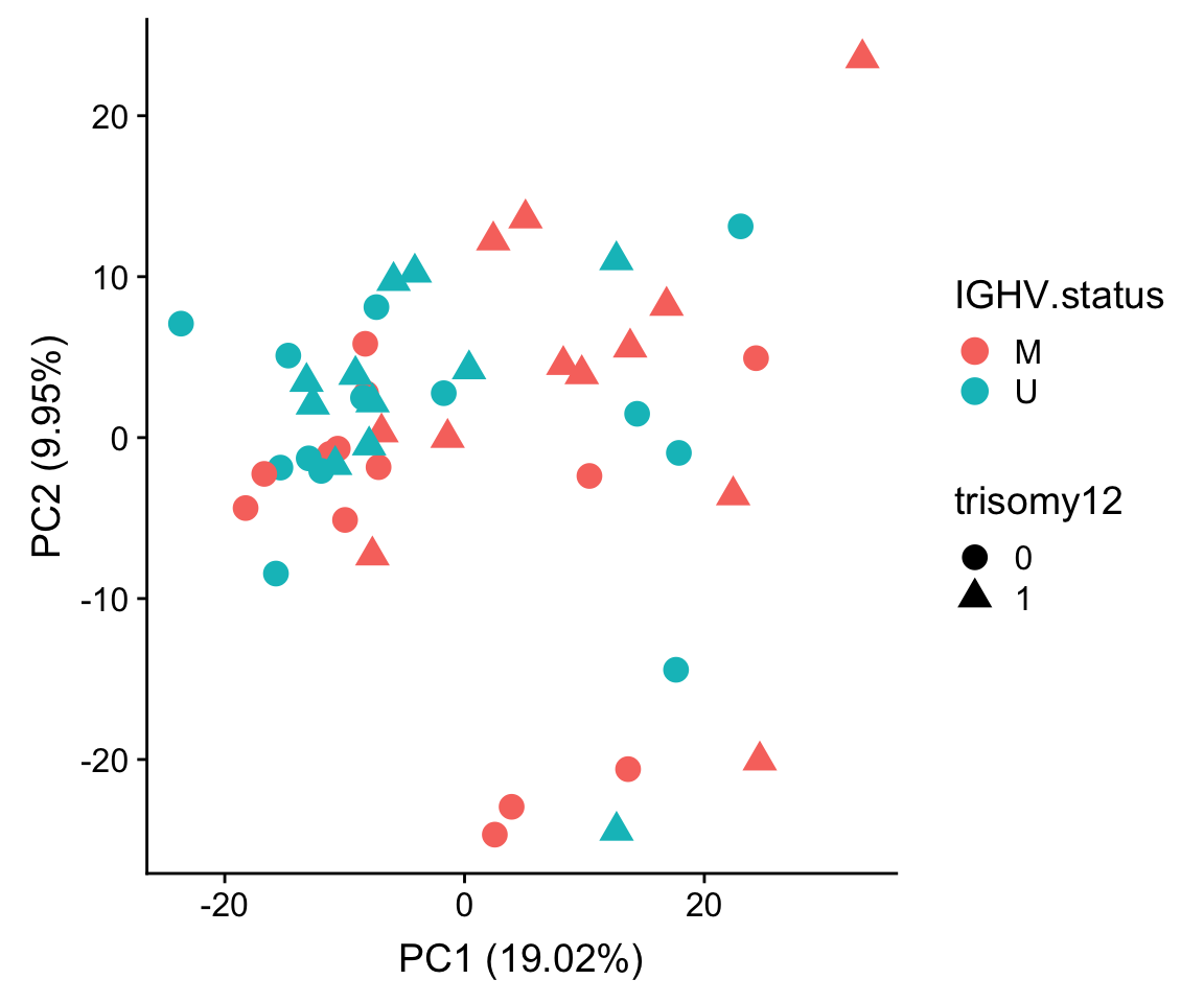
Plot PC3 and PC4
plotTab <- pcRes %>% data.frame() %>% cbind(colAnno[rownames(.),]) %>%
  rownames_to_column("patID") %>% as_tibble()

ggplot(plotTab, aes(x=PC3, y=PC4, col = IGHV.status, shape = trisomy12)) + geom_point(size=4) +
  xlab(sprintf("PC3 (%1.2f%%)",varExp[["PC3"]]*100)) +
  ylab(sprintf("PC4 (%1.2f%%)",varExp[["PC4"]]*100))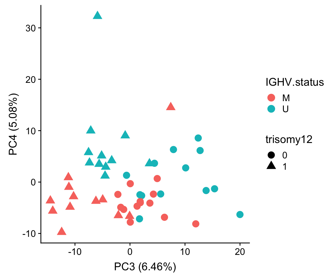
Plot PC4 and PC5
plotTab <- pcRes %>% data.frame() %>% cbind(colAnno[rownames(.),]) %>%
  rownames_to_column("patID") %>% as_tibble()

ggplot(plotTab, aes(x=PC4, y=PC5, col = IGHV.status, shape = trisomy12)) + geom_point(size=4) +
  xlab(sprintf("PC4 (%1.2f%%)",varExp[["PC4"]]*100)) +
  ylab(sprintf("PC5 (%1.2f%%)",varExp[["PC5"]]*100))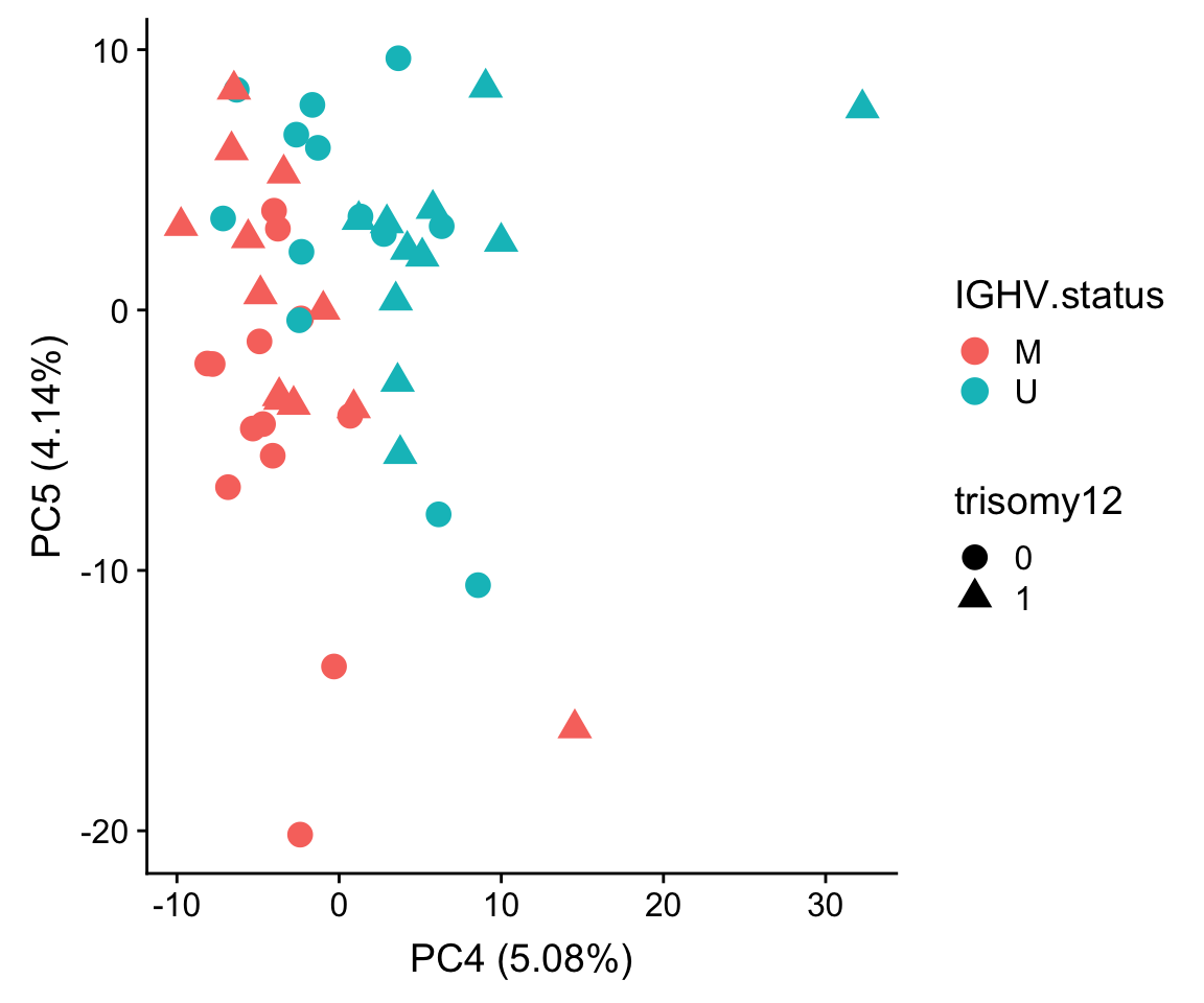
Correlation PCs with trisomy12 and IGHV status
corTab <- lapply(colnames(pcRes),  function(pc) {
  ighvCor <- t.test(pcRes[,pc] ~ colAnno$IGHV.status)
  tri12Cor <- t.test(pcRes[,pc] ~ colAnno$trisomy12)
  tibble(PC = pc,
         feature=c("IGHV", "trisomy12"),
         p = c(ighvCor$p.value, tri12Cor$p.value))
}) %>% bind_rows() %>% mutate(p.adj = p.adjust(p, method = "BH")) %>%
  filter(p <= 0.05) %>% arrange(p)
corTab
# A tibble: 4 x 4
PC feature p p.adj
<chr> <chr> <dbl> <dbl>
1 PC3 trisomy12 0.00000000812 0.000000795
2 PC4 IGHV 0.000368 0.0180
3 PC5 IGHV 0.00476 0.156
4 PC3 IGHV 0.0345 0.828 PC3 represents trisomy12 and PC4 represents IGHV. From another analysis, we know that PC5 represents CLL-PD.
Enrichment analysis on PCs
PC1
gmts = list(H= "../data/gmts/h.all.v6.2.symbols.gmt",
            KEGG = "../data/gmts/c2.cp.kegg.v6.2.symbols.gmt",
            C6 = "../data/gmts/c6.all.v6.2.symbols.gmt")
iPC <- "PC1"
proMat <- assays(protCLL.sub)[["QRILC"]]
pc <- pcRes[,iPC][colnames(proMat)]
designMat <- model.matrix(~1+pc)
res <- runCamera(proMat, designMat, gmts$H, id = rowData(protCLL[rownames(proMat),])$hgnc_symbol)Hallmarks
res <- runCamera(proMat, designMat, gmts$H, id = rowData(protCLL[rownames(proMat),])$hgnc_symbol)
res$enrichPlot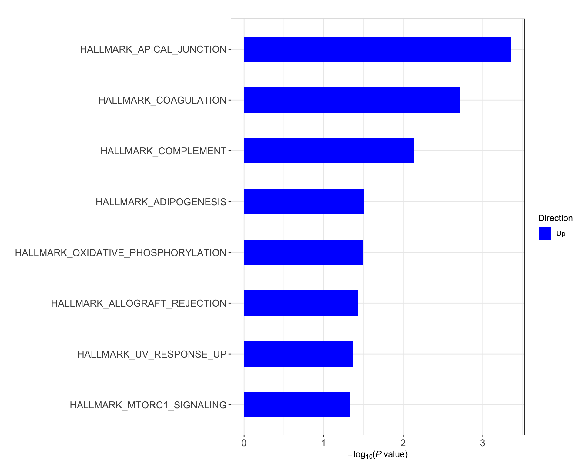
KEGG
res <- runCamera(proMat, designMat, gmts$KEGG, id = rowData(protCLL[rownames(proMat),])$hgnc_symbol)
res$enrichPlot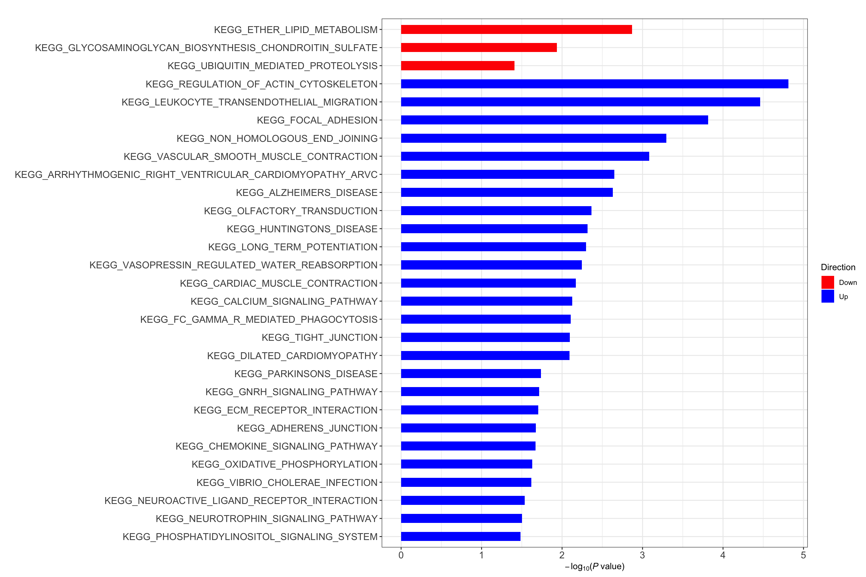
C6 oncogentic signatures
res <- runCamera(proMat, designMat, gmts$C6, id = rowData(protCLL[rownames(proMat),])$hgnc_symbol)
res$enrichPlot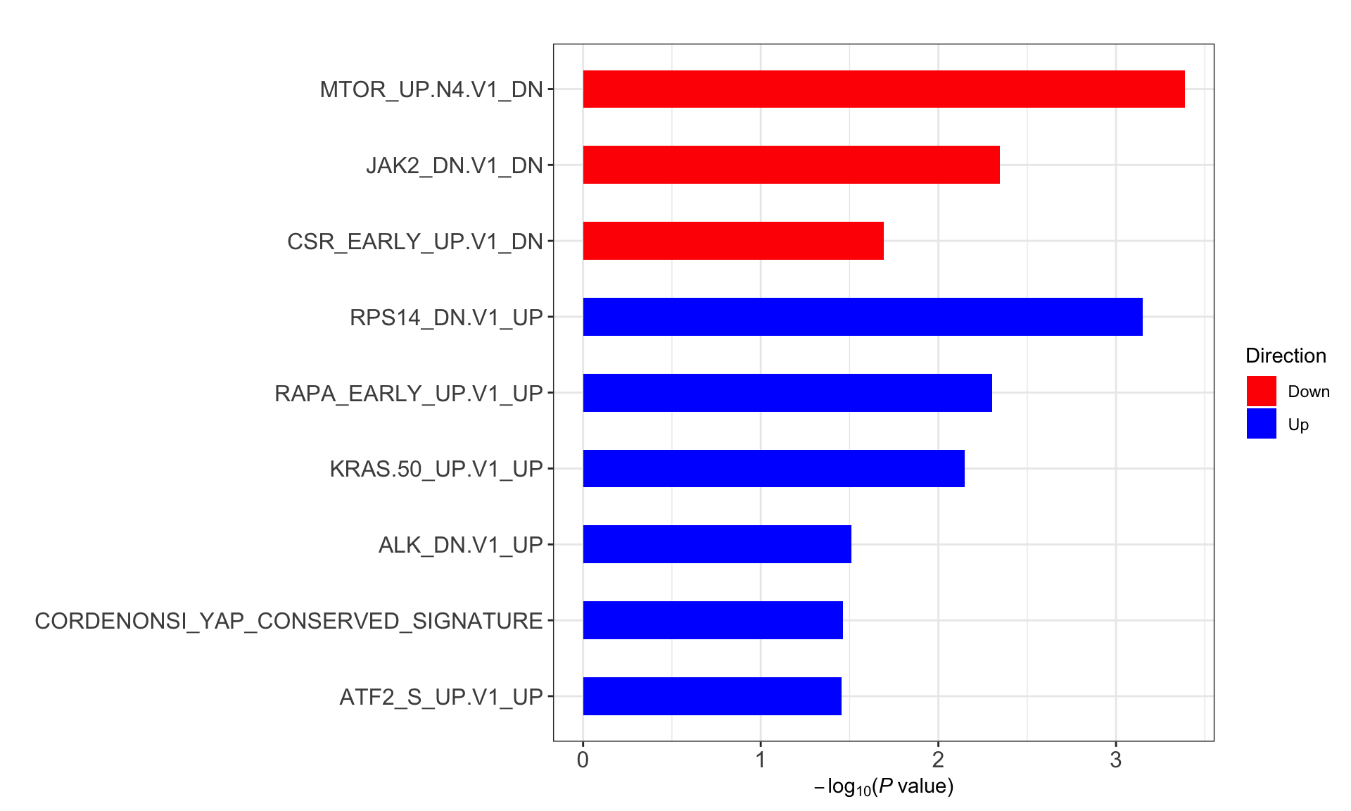
Proteins associated with PC1
fit <- lmFit(proMat,  designMat)
fit2 <- eBayes(fit)
corRes <- topTable(fit2, number ="all", adjust.method = "BH", coef = "pc") %>% rownames_to_column("id") %>%
    mutate(symbol = rowData(protCLL[id,])$hgnc_symbol)
Table of significant associations (5% FDR)
resTab.sig <- filter(corRes, adj.P.Val < 0.05) %>%
  select(symbol, id,logFC, P.Value, adj.P.Val) %>%
  arrange(P.Value)
resTab.sig %>% mutate_if(is.numeric, formatC, digits=2, format= "e") %>%
  DT::datatable()
Heatmap of top100 associated proteins
colAnno <- pcRes[colnames(proMat),iPC, drop= FALSE] %>% data.frame() %>%
  rownames_to_column("patID") %>%
  mutate(IGHV = protCLL[,patID]$IGHV.status,
         trisomy12 = protCLL[,patID]$trisomy12,
         TP53 = patMeta[match(patID, patMeta$Patient.ID),]$TP53,
         SF3B1 = patMeta[match(patID, patMeta$Patient.ID),]$SF3B1,
         NOTCH1 = patMeta[match(patID, patMeta$Patient.ID),]$NOTCH1) %>%
  arrange(!!rlang::sym(iPC)) %>% data.frame() %>% column_to_rownames("patID")

plotMat <- proMat[resTab.sig$id[1:100],rownames(colAnno)]
plotMat <- jyluMisc::mscale(plotMat, censor = 6)

pheatmap(plotMat, scale = "none", annotation_col = colAnno, clustering_method = "ward.D2",
         cluster_cols = FALSE,
         labels_row = resTab.sig$symbol[1:100], color = colorRampPalette(c("navy","white","firebrick"))(100),
         breaks = seq(-6,6, length.out = 101))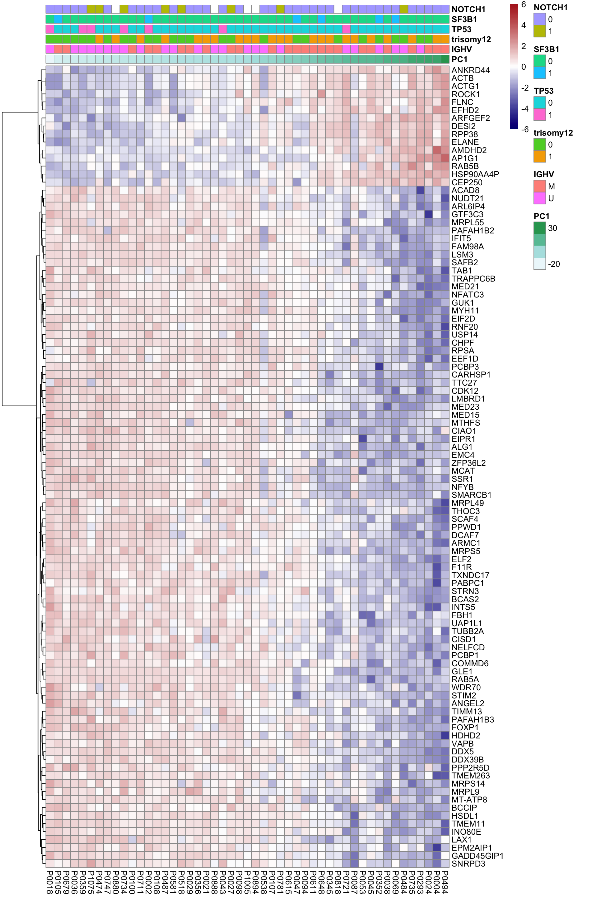
PC2
iPC <- "PC2"
proMat <- assays(protCLL.sub)[["QRILC"]]
pc <- pcRes[,iPC][colnames(proMat)]
designMat <- model.matrix(~1+pc)
res <- runCamera(proMat, designMat, gmts$H, id = rowData(protCLL[rownames(proMat),])$hgnc_symbol)
Hallmarks
res <- runCamera(proMat, designMat, gmts$H, id = rowData(protCLL[rownames(proMat),])$hgnc_symbol)
res$enrichPlot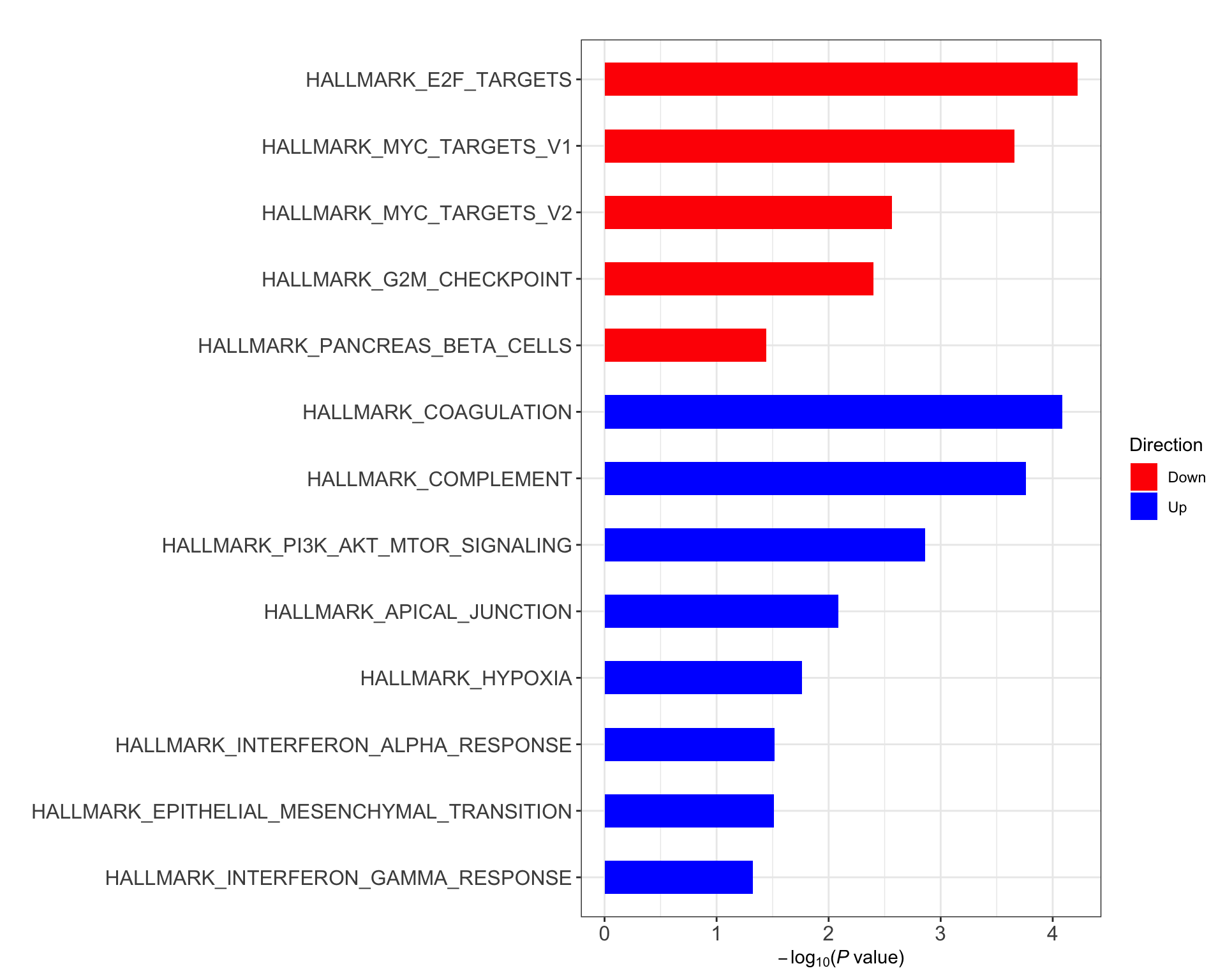
KEGG
res <- runCamera(proMat, designMat, gmts$KEGG, id = rowData(protCLL[rownames(proMat),])$hgnc_symbol)
res$enrichPlot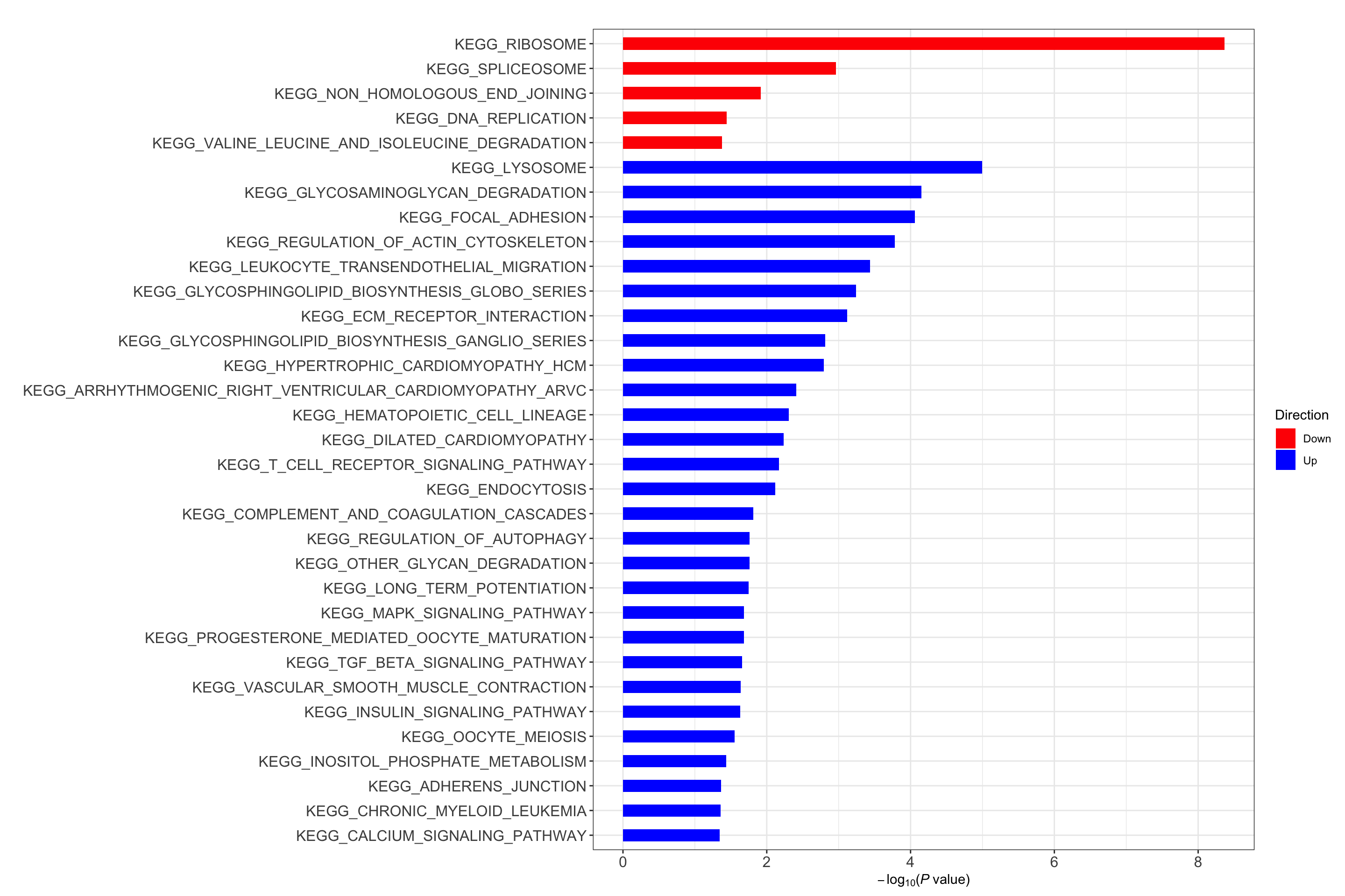
C6 oncogentic signatures
res <- runCamera(proMat, designMat, gmts$C6, id = rowData(protCLL[rownames(proMat),])$hgnc_symbol)
res$enrichPlot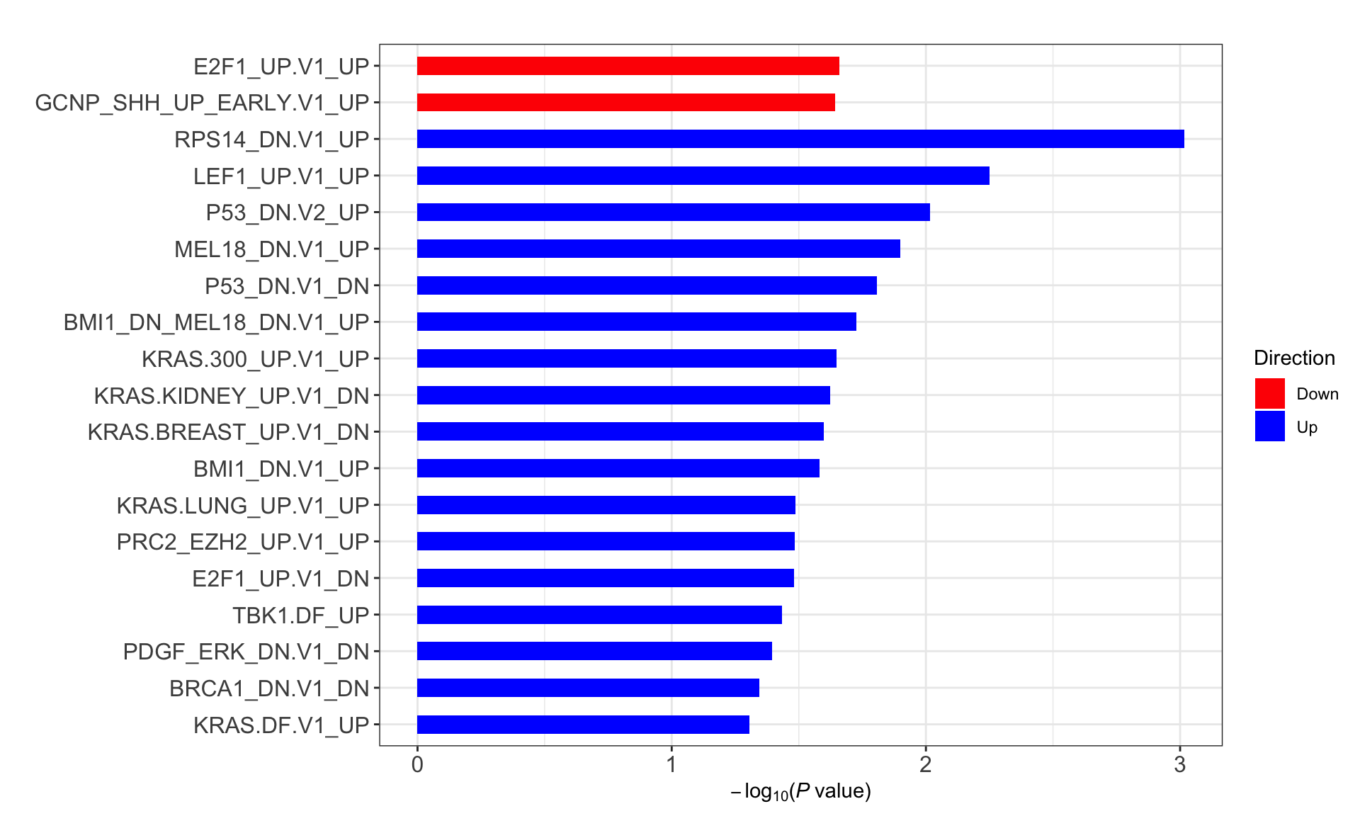
Proteins associated with PC2
fit <- lmFit(proMat,  designMat)
fit2 <- eBayes(fit)
corRes <- topTable(fit2, number ="all", adjust.method = "BH", coef = "pc") %>% rownames_to_column("id") %>%
    mutate(symbol = rowData(protCLL[id,])$hgnc_symbol)
Table of significant associations (5% FDR)
resTab.sig <- filter(corRes, adj.P.Val < 0.05) %>%
  select(symbol, id,logFC, P.Value, adj.P.Val) %>%
  arrange(P.Value)
resTab.sig %>% mutate_if(is.numeric, formatC, digits=2, format= "e") %>%
  DT::datatable()
Heatmap of top100 associated proteins
colAnno <- pcRes[colnames(proMat),iPC, drop= FALSE] %>% data.frame() %>%
  rownames_to_column("patID") %>%
  mutate(IGHV = protCLL[,patID]$IGHV.status,
         trisomy12 = protCLL[,patID]$trisomy12,
         TP53 = patMeta[match(patID, patMeta$Patient.ID),]$TP53,
         SF3B1 = patMeta[match(patID, patMeta$Patient.ID),]$SF3B1,
         NOTCH1 = patMeta[match(patID, patMeta$Patient.ID),]$NOTCH1) %>%
  arrange(!!rlang::sym(iPC)) %>% data.frame() %>% column_to_rownames("patID")

plotMat <- proMat[resTab.sig$id[1:100],rownames(colAnno)]
plotMat <- jyluMisc::mscale(plotMat, censor = 6)

pheatmap(plotMat, scale = "none", annotation_col = colAnno, clustering_method = "ward.D2",
         cluster_cols = FALSE,
         labels_row = resTab.sig$symbol[1:100], color = colorRampPalette(c("navy","white","firebrick"))(100),
         breaks = seq(-6,6, length.out = 101))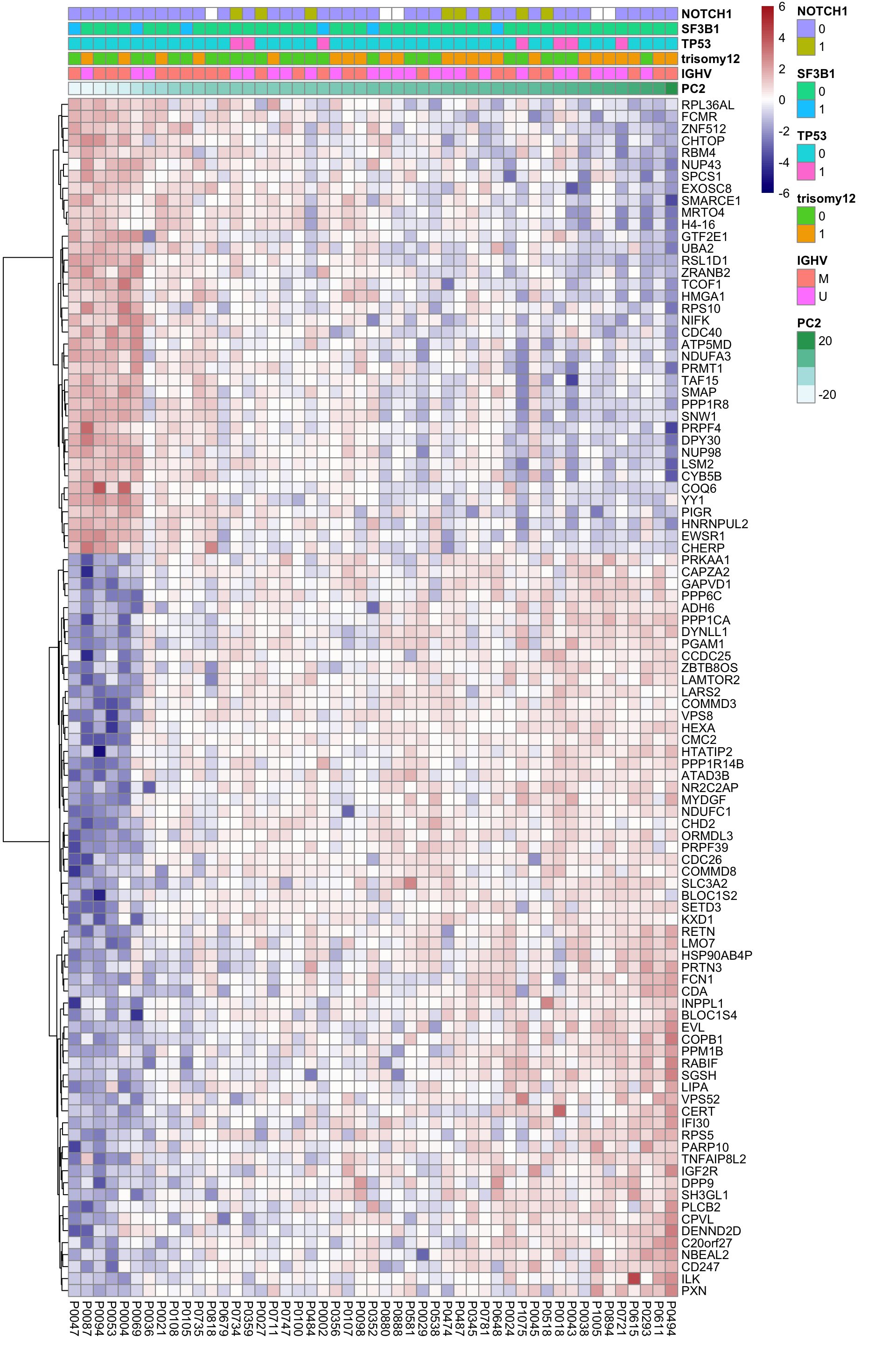
PC3
iPC <- "PC3"
proMat <- assays(protCLL.sub)[["QRILC"]]
pc <- pcRes[,iPC][colnames(proMat)]
designMat <- model.matrix(~1+pc)
res <- runCamera(proMat, designMat, gmts$H, id = rowData(protCLL[rownames(proMat),])$hgnc_symbol)
Hallmarks
res <- runCamera(proMat, designMat, gmts$H, id = rowData(protCLL[rownames(proMat),])$hgnc_symbol)
res$enrichPlot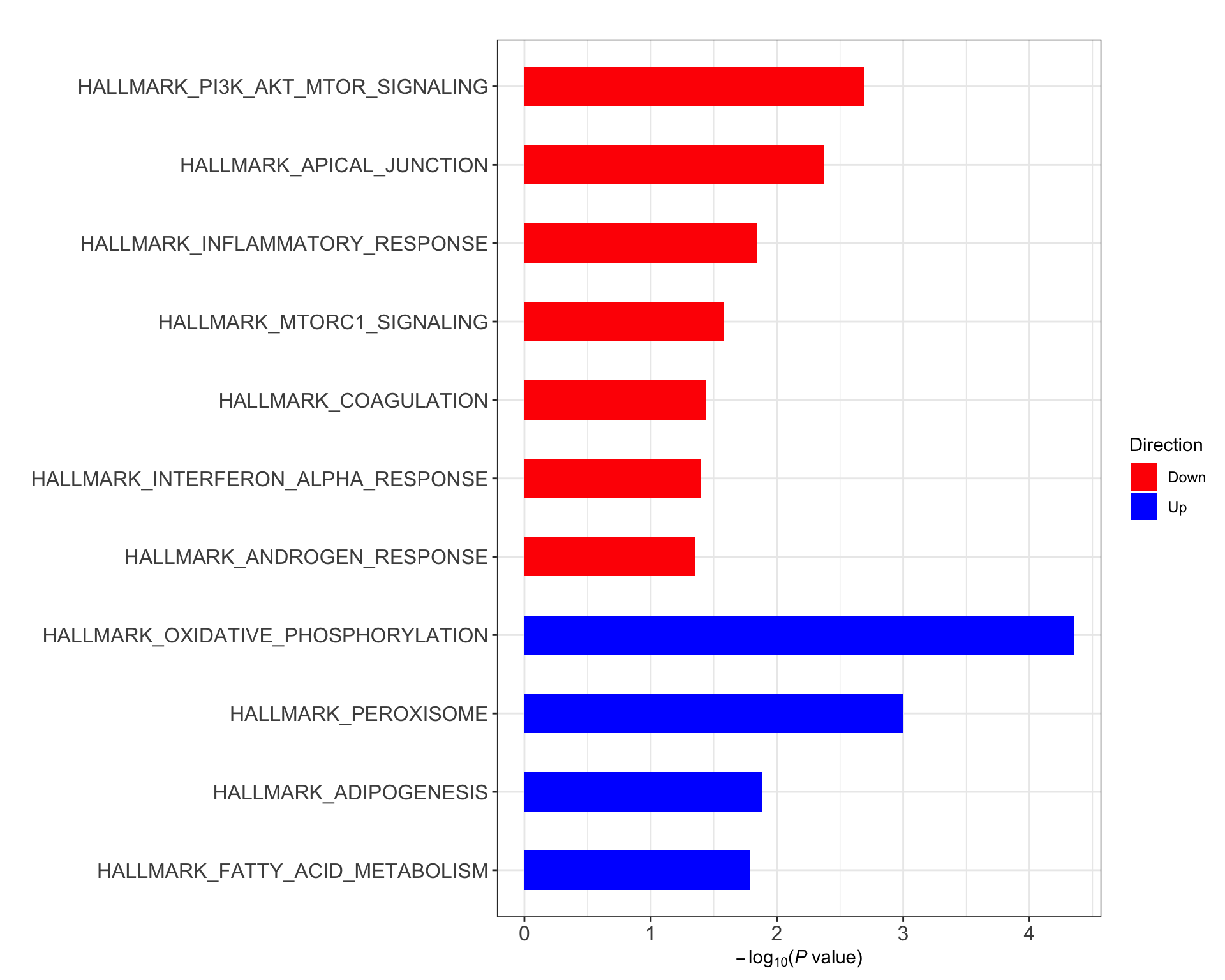
KEGG
res <- runCamera(proMat, designMat, gmts$KEGG, id = rowData(protCLL[rownames(proMat),])$hgnc_symbol)
res$enrichPlot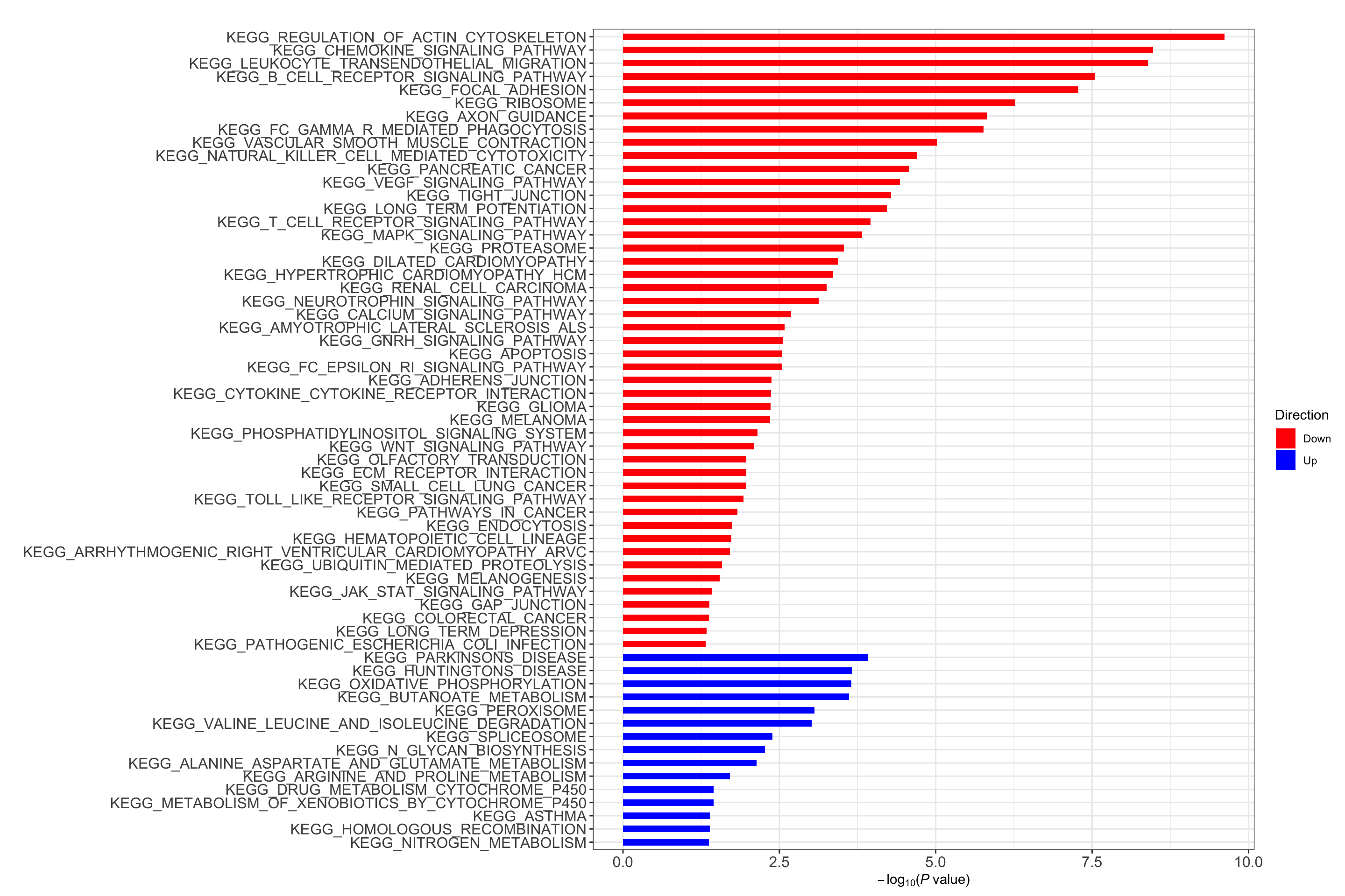
C6 oncogentic signatures
res <- runCamera(proMat, designMat, gmts$C6, id = rowData(protCLL[rownames(proMat),])$hgnc_symbol)
res$enrichPlot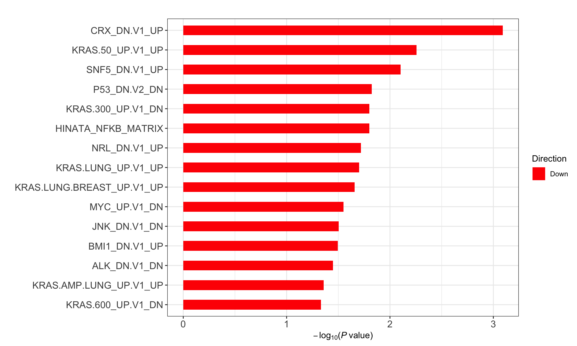
Proteins associated with PC3
fit <- lmFit(proMat,  designMat)
fit2 <- eBayes(fit)
corRes <- topTable(fit2, number ="all", adjust.method = "BH", coef = "pc") %>% rownames_to_column("id") %>%
    mutate(symbol = rowData(protCLL[id,])$hgnc_symbol)
Table of significant associations (5% FDR)
resTab.sig <- filter(corRes, adj.P.Val < 0.05) %>%
  select(symbol, id,logFC, P.Value, adj.P.Val) %>%
  arrange(P.Value)
resTab.sig %>% mutate_if(is.numeric, formatC, digits=2, format= "e") %>%
  DT::datatable()
Heatmap of top100 associated proteins
colAnno <- pcRes[colnames(proMat),iPC, drop= FALSE] %>% data.frame() %>%
  rownames_to_column("patID") %>%
  mutate(IGHV = protCLL[,patID]$IGHV.status,
         trisomy12 = protCLL[,patID]$trisomy12,
         TP53 = patMeta[match(patID, patMeta$Patient.ID),]$TP53,
         SF3B1 = patMeta[match(patID, patMeta$Patient.ID),]$SF3B1,
         NOTCH1 = patMeta[match(patID, patMeta$Patient.ID),]$NOTCH1) %>%
  arrange(!!rlang::sym(iPC)) %>% data.frame() %>% column_to_rownames("patID")
plotMat <- proMat[resTab.sig$id[1:100],rownames(colAnno)]
plotMat <- jyluMisc::mscale(plotMat, censor = 6)

pheatmap(plotMat, scale = "none", annotation_col = colAnno, clustering_method = "ward.D2",
         cluster_cols = FALSE,
         labels_row = resTab.sig$symbol[1:100], color = colorRampPalette(c("navy","white","firebrick"))(100),
         breaks = seq(-6,6, length.out = 101))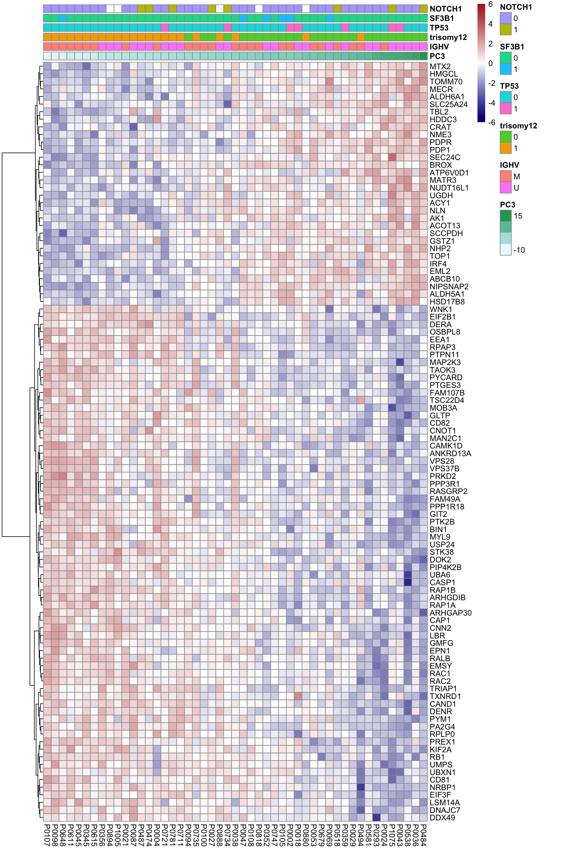
PC4
iPC <- "PC4"
proMat <- assays(protCLL.sub)[["QRILC"]]
pc <- pcRes[,iPC][colnames(proMat)]
designMat <- model.matrix(~1+pc)
res <- runCamera(proMat, designMat, gmts$H, id = rowData(protCLL[rownames(proMat),])$hgnc_symbol)
Hallmarks
res <- runCamera(proMat, designMat, gmts$H, id = rowData(protCLL[rownames(proMat),])$hgnc_symbol)
res$enrichPlot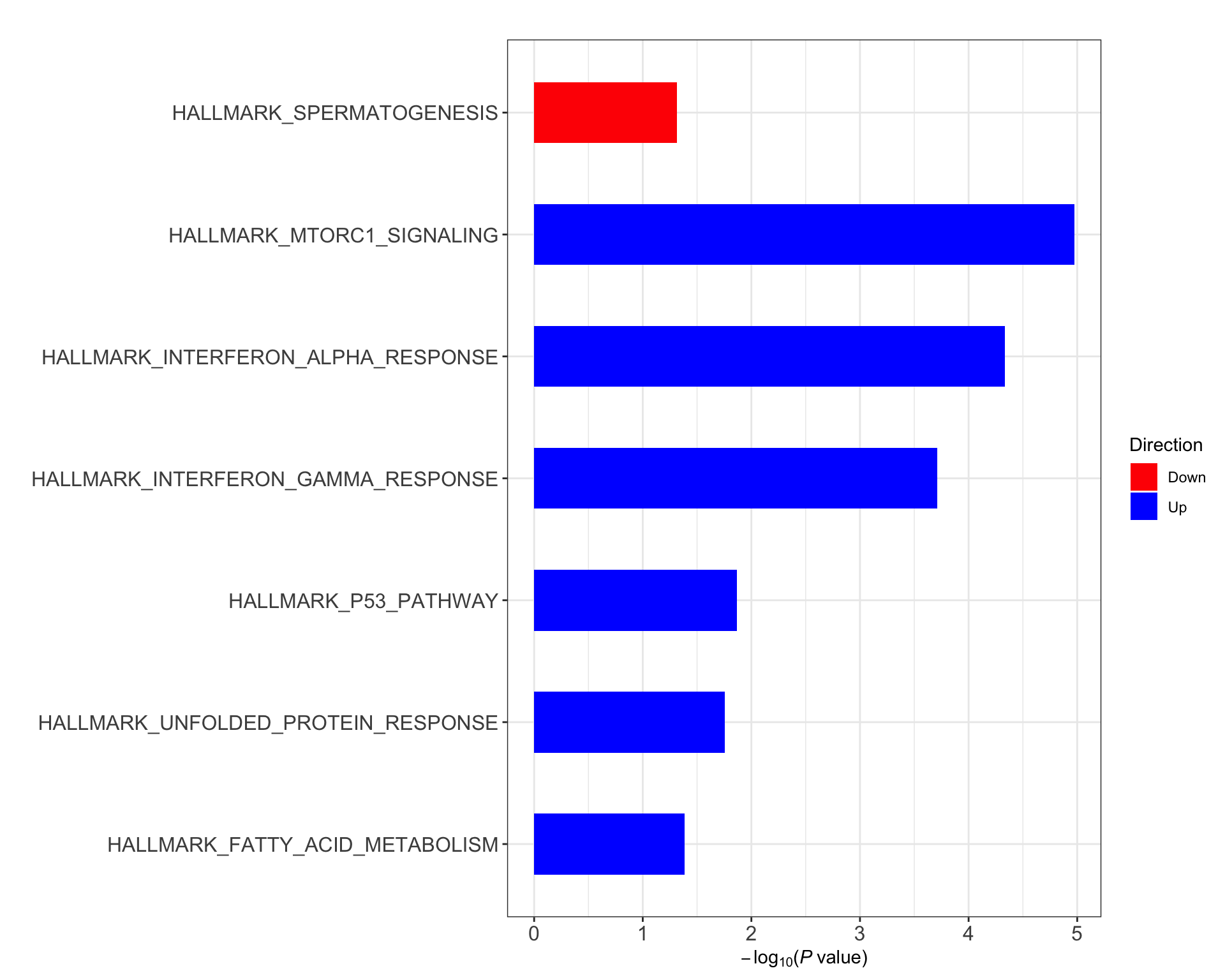
KEGG
res <- runCamera(proMat, designMat, gmts$KEGG, id = rowData(protCLL[rownames(proMat),])$hgnc_symbol)
res$enrichPlot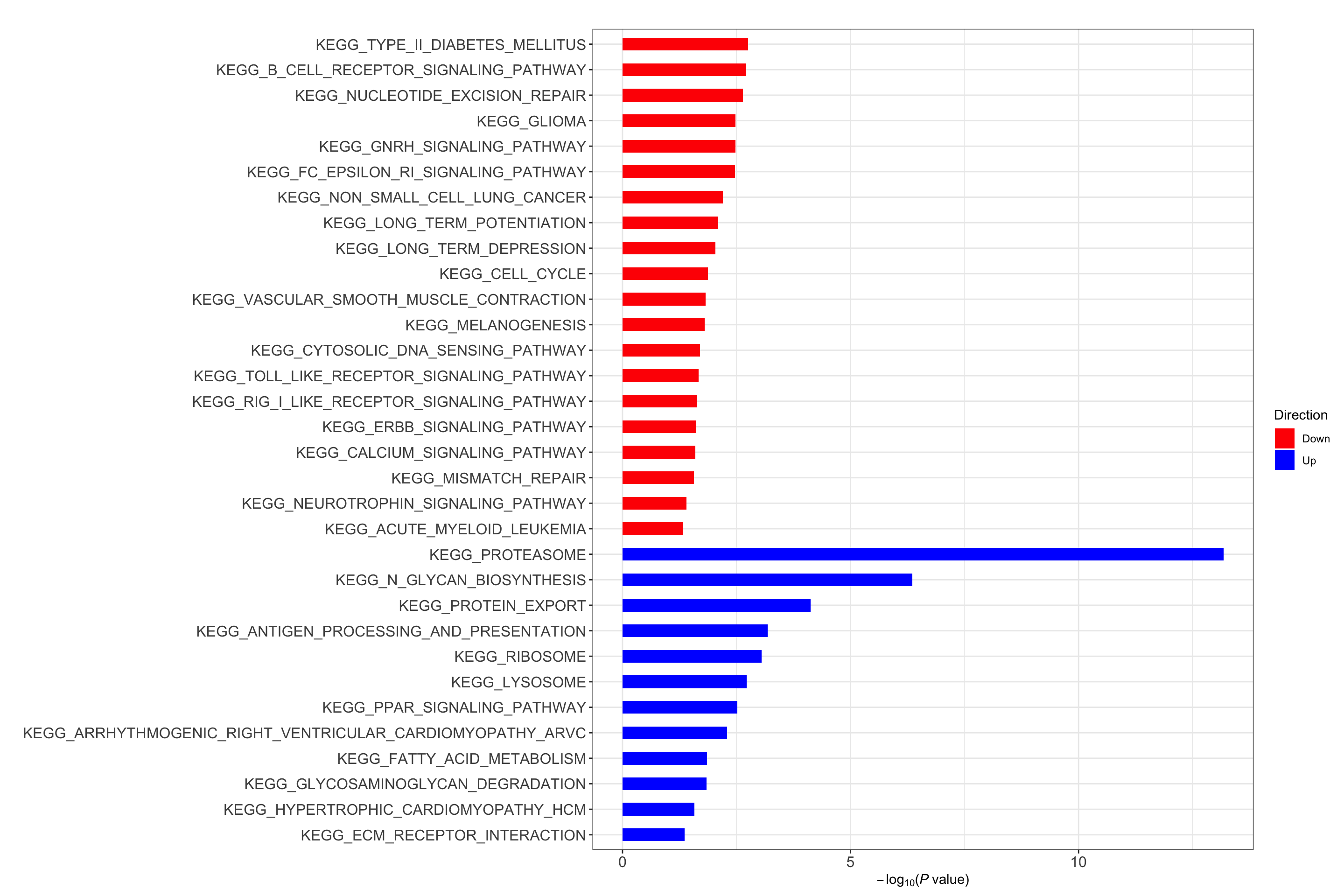
C6 oncogentic signatures
res <- runCamera(proMat, designMat, gmts$C6, id = rowData(protCLL[rownames(proMat),])$hgnc_symbol)
res$enrichPlot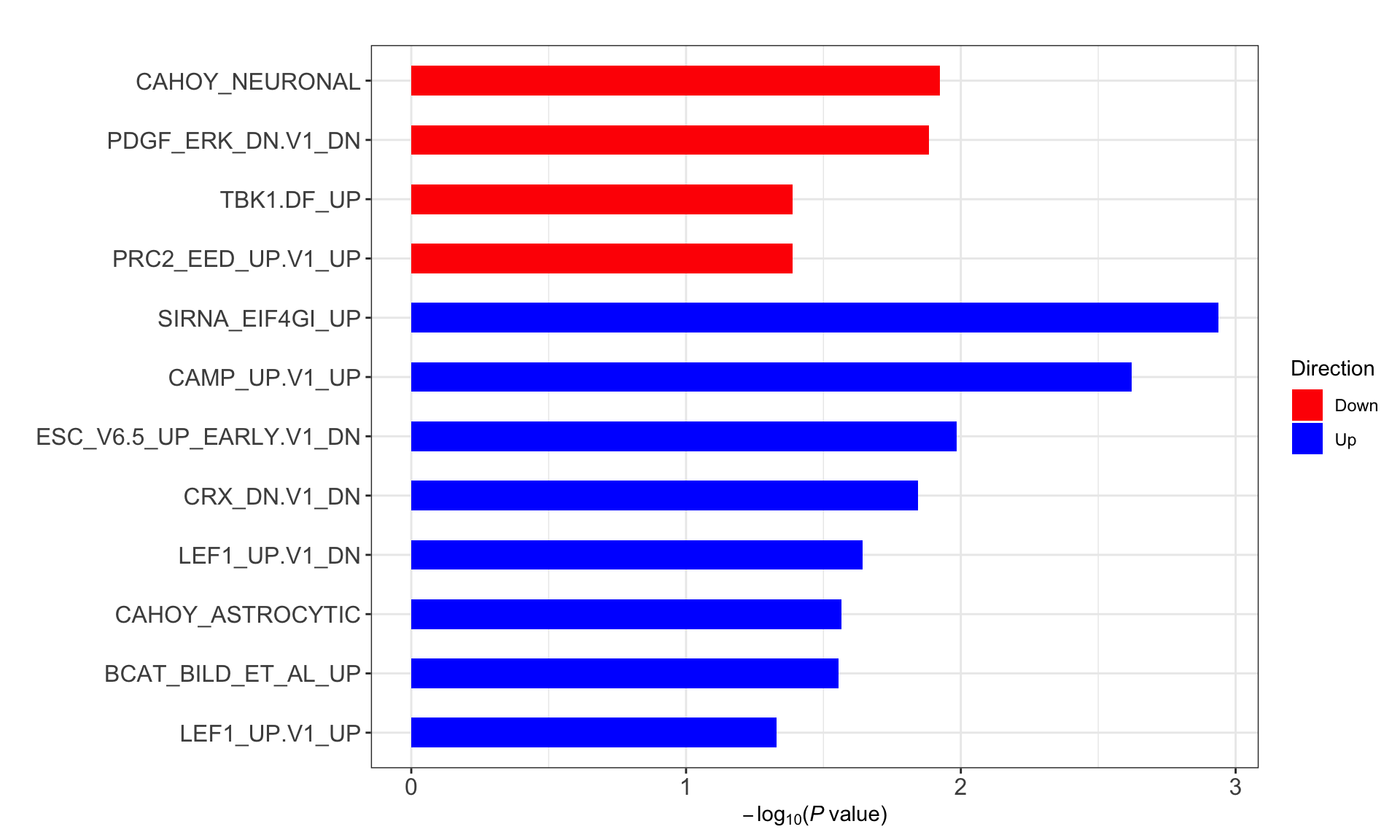
Proteins associated with PC4
fit <- lmFit(proMat,  designMat)
fit2 <- eBayes(fit)
corRes <- topTable(fit2, number ="all", adjust.method = "BH", coef = "pc") %>% rownames_to_column("id") %>%
    mutate(symbol = rowData(protCLL[id,])$hgnc_symbol)
Table of significant associations (5% FDR)
resTab.sig <- filter(corRes, adj.P.Val < 0.05) %>%
  select(symbol, id,logFC, P.Value, adj.P.Val) %>%
  arrange(P.Value)
resTab.sig %>% mutate_if(is.numeric, formatC, digits=2, format= "e") %>%
  DT::datatable()
Heatmap of top100 associated proteins
colAnno <- pcRes[colnames(proMat),iPC, drop= FALSE] %>% data.frame() %>%
  rownames_to_column("patID") %>%
  mutate(IGHV = protCLL[,patID]$IGHV.status,
         trisomy12 = protCLL[,patID]$trisomy12,
         TP53 = patMeta[match(patID, patMeta$Patient.ID),]$TP53,
         SF3B1 = patMeta[match(patID, patMeta$Patient.ID),]$SF3B1,
         NOTCH1 = patMeta[match(patID, patMeta$Patient.ID),]$NOTCH1) %>%
  arrange(!!rlang::sym(iPC)) %>% data.frame() %>% column_to_rownames("patID")

plotMat <- proMat[resTab.sig$id[1:100],rownames(colAnno)]
plotMat <- jyluMisc::mscale(plotMat, censor = 6)

pheatmap(plotMat, scale = "none", annotation_col = colAnno, clustering_method = "ward.D2",
         cluster_cols = FALSE,
         labels_row = resTab.sig$symbol[1:100], color = colorRampPalette(c("navy","white","firebrick"))(100),
         breaks = seq(-6,6, length.out = 101))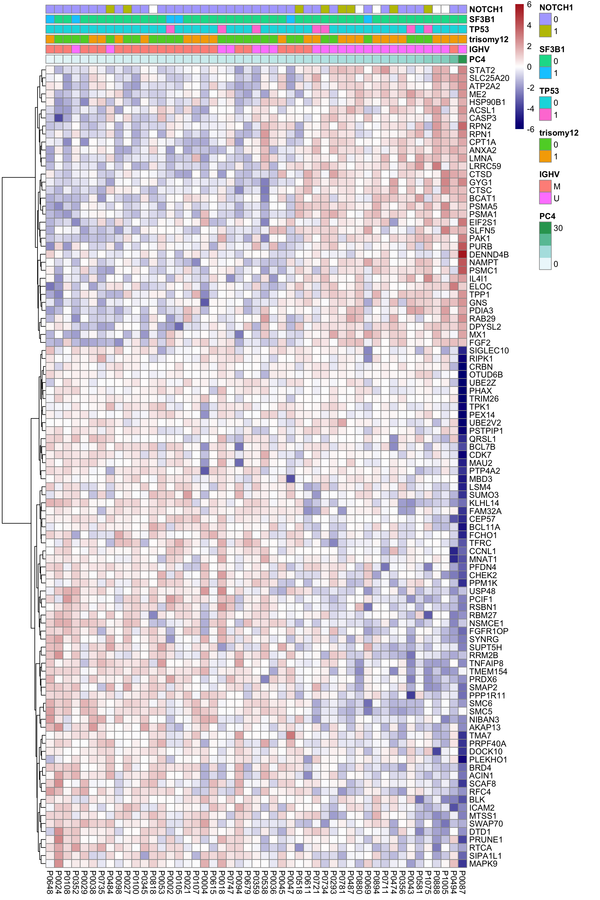
PC5
iPC <- "PC5"
proMat <- assays(protCLL.sub)[["QRILC"]]
pc <- pcRes[,iPC][colnames(proMat)]
designMat <- model.matrix(~1+pc)
res <- runCamera(proMat, designMat, gmts$H, id = rowData(protCLL[rownames(proMat),])$hgnc_symbol)
Hallmarks
res <- runCamera(proMat, designMat, gmts$H, id = rowData(protCLL[rownames(proMat),])$hgnc_symbol)
res$enrichPlot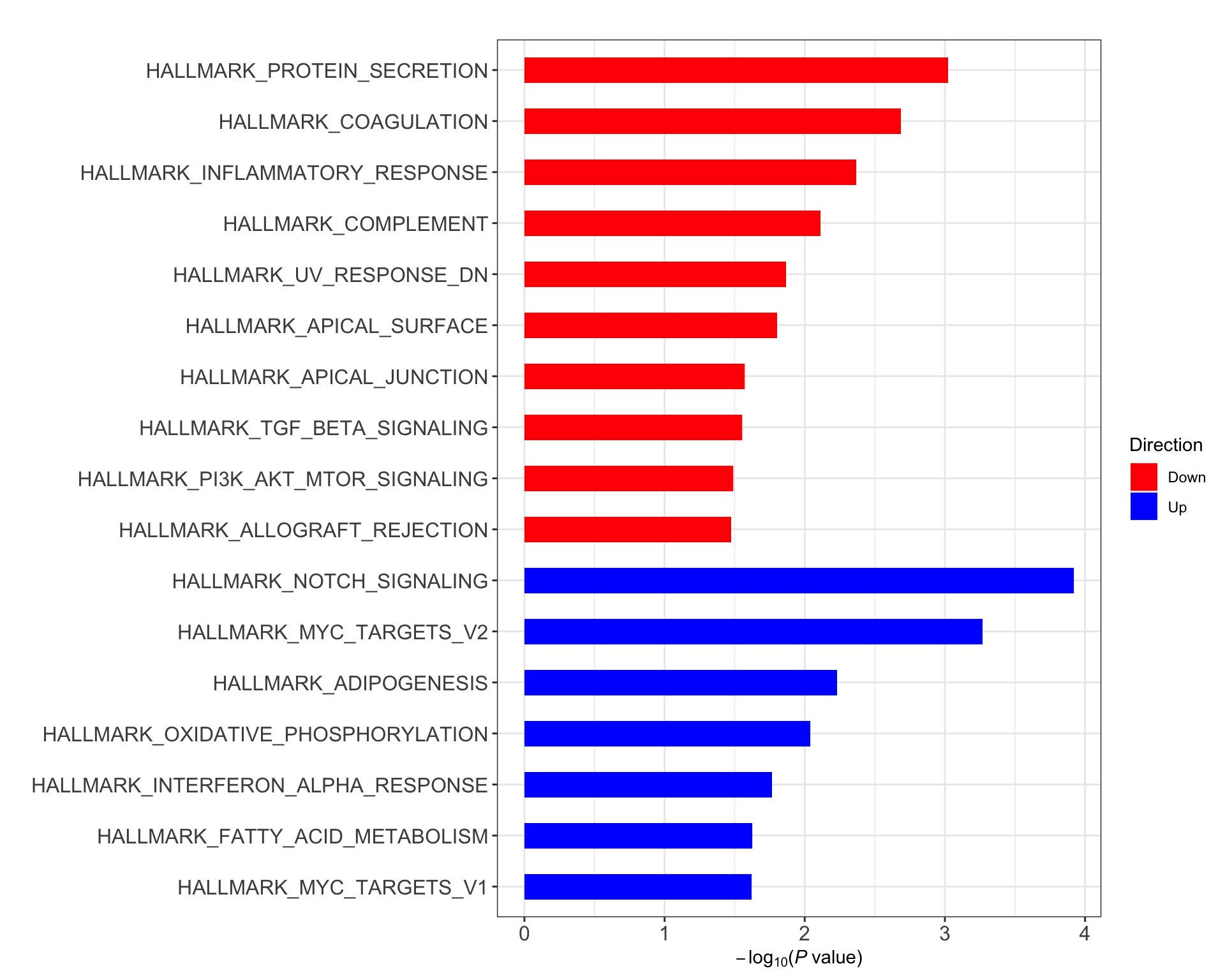
KEGG
res <- runCamera(proMat, designMat, gmts$KEGG, id = rowData(protCLL[rownames(proMat),])$hgnc_symbol)
res$enrichPlot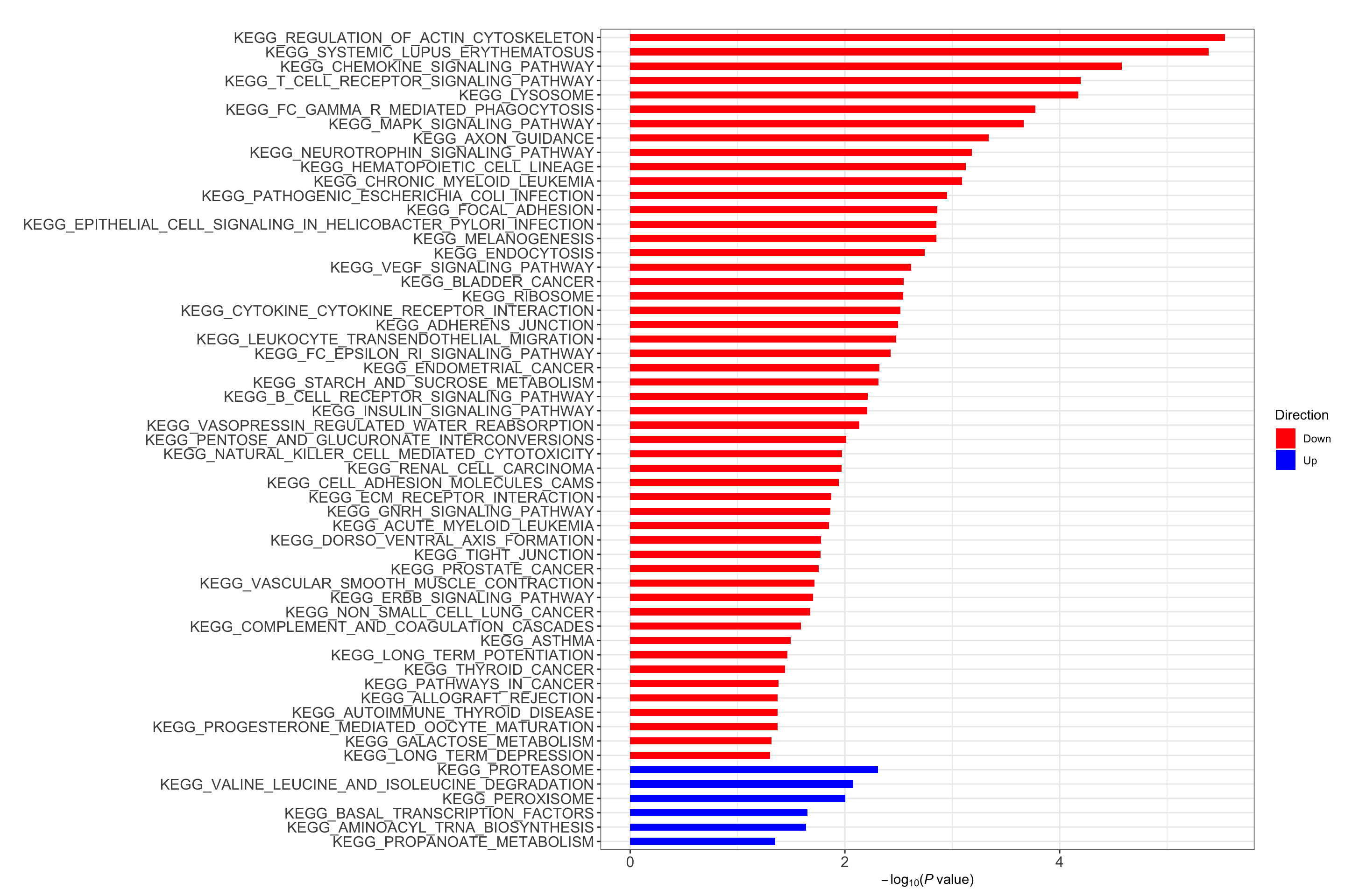
C6 oncogentic signatures
res <- runCamera(proMat, designMat, gmts$C6, id = rowData(protCLL[rownames(proMat),])$hgnc_symbol)
res$enrichPlot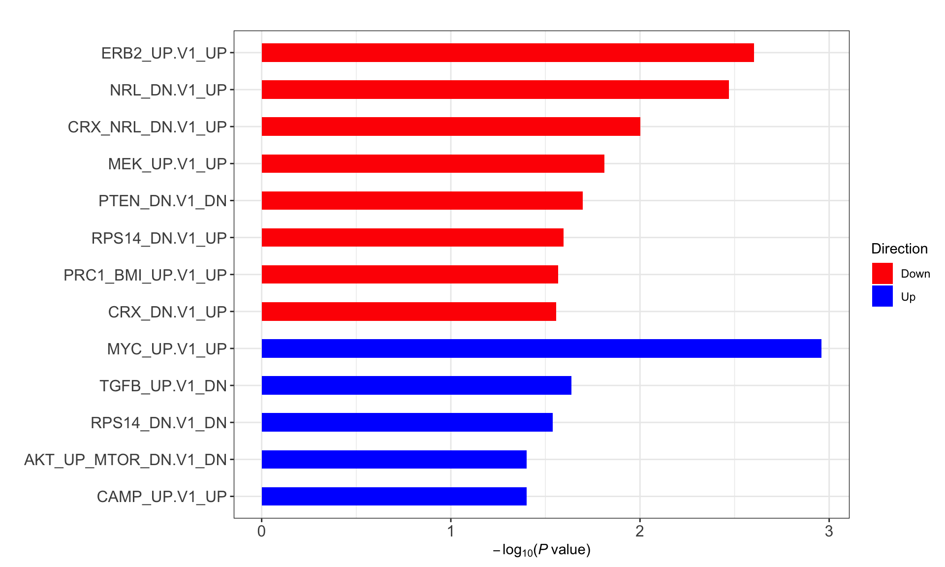
Proteins associated with PC5
fit <- lmFit(proMat,  designMat)
fit2 <- eBayes(fit)
corRes <- topTable(fit2, number ="all", adjust.method = "BH", coef = "pc") %>% rownames_to_column("id") %>%
    mutate(symbol = rowData(protCLL[id,])$hgnc_symbol)
Table of significant associations (5% FDR)
resTab.sig <- filter(corRes, adj.P.Val < 0.05) %>%
  select(symbol, id,logFC, P.Value, adj.P.Val) %>%
  arrange(P.Value)
resTab.sig %>% mutate_if(is.numeric, formatC, digits=2, format= "e") %>%
  DT::datatable()
Heatmap of top100 associated proteins
colAnno <- pcRes[colnames(proMat),iPC, drop= FALSE] %>% data.frame() %>%
  rownames_to_column("patID") %>%
  mutate(IGHV = protCLL[,patID]$IGHV.status,
         trisomy12 = protCLL[,patID]$trisomy12,
         TP53 = patMeta[match(patID, patMeta$Patient.ID),]$TP53,
         SF3B1 = patMeta[match(patID, patMeta$Patient.ID),]$SF3B1,
         NOTCH1 = patMeta[match(patID, patMeta$Patient.ID),]$NOTCH1) %>%
  arrange(!!rlang::sym(iPC)) %>% data.frame() %>% column_to_rownames("patID")
plotMat <- proMat[resTab.sig$id[1:100],rownames(colAnno)]
plotMat <- jyluMisc::mscale(plotMat, censor = 6)

pheatmap(plotMat, scale = "none", annotation_col = colAnno, clustering_method = "ward.D2",
         cluster_cols = FALSE,
         labels_row = resTab.sig$symbol[1:100], color = colorRampPalette(c("navy","white","firebrick"))(100),
         breaks = seq(-6,6, length.out = 101))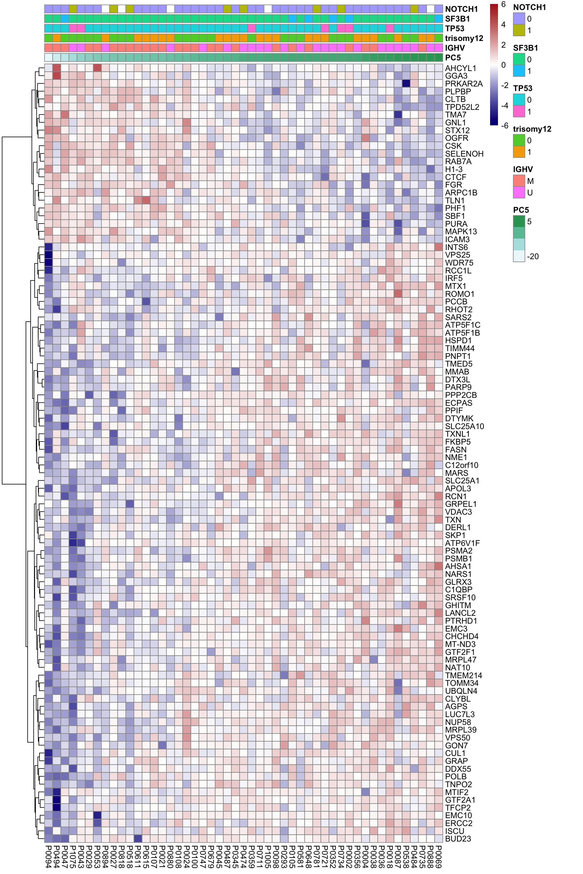
sessionInfo()R version 3.6.0 (2019-04-26)
Platform: x86_64-apple-darwin15.6.0 (64-bit)
Running under: macOS 10.15.4
Matrix products: default
BLAS: /Library/Frameworks/R.framework/Versions/3.6/Resources/lib/libRblas.0.dylib
LAPACK: /Library/Frameworks/R.framework/Versions/3.6/Resources/lib/libRlapack.dylib
locale:
[1] en_US.UTF-8/en_US.UTF-8/en_US.UTF-8/C/en_US.UTF-8/en_US.UTF-8
attached base packages:
[1] parallel stats4 stats graphics grDevices utils datasets
[8] methods base
other attached packages:
[1] forcats_0.4.0 stringr_1.4.0
[3] dplyr_0.8.5 purrr_0.3.3
[5] readr_1.3.1 tidyr_1.0.0
[7] tibble_3.0.0 tidyverse_1.3.0
[9] SummarizedExperiment_1.14.0 DelayedArray_0.10.0
[11] BiocParallel_1.18.0 matrixStats_0.54.0
[13] Biobase_2.44.0 GenomicRanges_1.36.0
[15] GenomeInfoDb_1.20.0 IRanges_2.18.1
[17] S4Vectors_0.22.0 BiocGenerics_0.30.0
[19] limma_3.40.2 jyluMisc_0.1.5
[21] pheatmap_1.0.12 piano_2.0.2
[23] cowplot_0.9.4 ggplot2_3.3.0
loaded via a namespace (and not attached):
[1] readxl_1.3.1 backports_1.1.4 fastmatch_1.1-0
[4] drc_3.0-1 workflowr_1.6.0 igraph_1.2.4.1
[7] shinydashboard_0.7.1 splines_3.6.0 crosstalk_1.0.0
[10] TH.data_1.0-10 digest_0.6.19 htmltools_0.4.0
[13] fansi_0.4.0 gdata_2.18.0 memoise_1.1.0
[16] magrittr_1.5 cluster_2.1.0 openxlsx_4.1.0.1
[19] annotate_1.62.0 modelr_0.1.5 sandwich_2.5-1
[22] colorspace_1.4-1 blob_1.1.1 rvest_0.3.5
[25] haven_2.2.0 xfun_0.8 crayon_1.3.4
[28] RCurl_1.95-4.12 jsonlite_1.6 genefilter_1.66.0
[31] survival_2.44-1.1 zoo_1.8-6 glue_1.3.2
[34] survminer_0.4.4 gtable_0.3.0 zlibbioc_1.30.0
[37] XVector_0.24.0 car_3.0-3 abind_1.4-5
[40] scales_1.1.0 mvtnorm_1.0-11 DBI_1.0.0
[43] relations_0.6-8 Rcpp_1.0.1 plotrix_3.7-6
[46] xtable_1.8-4 cmprsk_2.2-8 bit_1.1-14
[49] foreign_0.8-71 km.ci_0.5-2 DT_0.7
[52] htmlwidgets_1.3 httr_1.4.1 fgsea_1.10.0
[55] gplots_3.0.1.1 RColorBrewer_1.1-2 ellipsis_0.2.0
[58] farver_2.0.3 XML_3.98-1.20 pkgconfig_2.0.2
[61] dbplyr_1.4.2 utf8_1.1.4 labeling_0.3
[64] AnnotationDbi_1.46.0 tidyselect_1.0.0 rlang_0.4.5
[67] later_0.8.0 munsell_0.5.0 cellranger_1.1.0
[70] tools_3.6.0 visNetwork_2.0.7 cli_1.1.0
[73] RSQLite_2.1.1 generics_0.0.2 broom_0.5.2
[76] evaluate_0.14 yaml_2.2.0 bit64_0.9-7
[79] knitr_1.23 fs_1.4.0 zip_2.0.2
[82] survMisc_0.5.5 caTools_1.17.1.2 nlme_3.1-140
[85] mime_0.7 slam_0.1-45 xml2_1.2.2
[88] rstudioapi_0.10 compiler_3.6.0 curl_3.3
[91] ggsignif_0.5.0 marray_1.62.0 reprex_0.3.0
[94] stringi_1.4.3 lattice_0.20-38 Matrix_1.2-17
[97] shinyjs_1.0 KMsurv_0.1-5 vctrs_0.2.4
[100] pillar_1.4.3 lifecycle_0.2.0 data.table_1.12.2
[103] bitops_1.0-6 httpuv_1.5.1 R6_2.4.0
[106] promises_1.0.1 KernSmooth_2.23-15 gridExtra_2.3
[109] rio_0.5.16 codetools_0.2-16 MASS_7.3-51.4
[112] gtools_3.8.1 exactRankTests_0.8-30 assertthat_0.2.1
[115] rprojroot_1.3-2 withr_2.1.2 multcomp_1.4-10
[118] GenomeInfoDbData_1.2.1 hms_0.5.2 grid_3.6.0
[121] rmarkdown_1.13 carData_3.0-2 git2r_0.26.1
[124] maxstat_0.7-25 ggpubr_0.2.1 sets_1.0-18
[127] shiny_1.3.2 lubridate_1.7.4