Section 2: Identifying proteins associated disease drivers in CLL
Junyan Lu
2021-02-16
Last updated: 2021-02-16
Checks: 6 1
Knit directory: CLLproteomics_batch13/analysis/
This reproducible R Markdown analysis was created with workflowr (version 1.6.2). The Checks tab describes the reproducibility checks that were applied when the results were created. The Past versions tab lists the development history.
The R Markdown is untracked by Git. To know which version of the R Markdown file created these results, you'll want to first commit it to the Git repo. If you're still working on the analysis, you can ignore this warning. When you're finished, you can run wflow_publish to commit the R Markdown file and build the HTML.
Great job! The global environment was empty. Objects defined in the global environment can affect the analysis in your R Markdown file in unknown ways. For reproduciblity it's best to always run the code in an empty environment.
The command set.seed(20200227) was run prior to running the code in the R Markdown file. Setting a seed ensures that any results that rely on randomness, e.g. subsampling or permutations, are reproducible.
Great job! Recording the operating system, R version, and package versions is critical for reproducibility.
Nice! There were no cached chunks for this analysis, so you can be confident that you successfully produced the results during this run.
Great job! Using relative paths to the files within your workflowr project makes it easier to run your code on other machines.
Great! You are using Git for version control. Tracking code development and connecting the code version to the results is critical for reproducibility.
The results in this page were generated with repository version 3fb50c5. See the Past versions tab to see a history of the changes made to the R Markdown and HTML files.
Note that you need to be careful to ensure that all relevant files for the analysis have been committed to Git prior to generating the results (you can use wflow_publish or wflow_git_commit). workflowr only checks the R Markdown file, but you know if there are other scripts or data files that it depends on. Below is the status of the Git repository when the results were generated:
Ignored files:
    Ignored:    .DS_Store
    Ignored:    .Rhistory
    Ignored:    .Rproj.user/
    Ignored:    analysis/.DS_Store
    Ignored:    analysis/.Rhistory
    Ignored:    analysis/compareTreatment_cache/
    Ignored:    analysis/manuscript_S1_Overview_cache/
    Ignored:    analysis/manuscript_S3_trisomy12_cache/
    Ignored:    analysis/manuscript_S4_trisomy19_cache/
    Ignored:    analysis/manuscript_S5_IGHV_cache/
    Ignored:    analysis/manuscript_S6_del11q_cache/
    Ignored:    analysis/manuscript_S7_SF3B1_cache/
    Ignored:    analysis/manuscript_S8_drugResponse_Outcomes_cache/
    Ignored:    analysis/manuscript_S9_STAT2_cache/
    Ignored:    code/.DS_Store
    Ignored:    code/.Rhistory
    Ignored:    data/.DS_Store
    Ignored:    output/.DS_Store

Untracked files:
    Untracked:  analysis/.trisomy12_norm.pdf
    Untracked:  analysis/analysisBatch2.Rmd
    Untracked:  analysis/bufferAnalysis.Rmd
    Untracked:  analysis/compareTreatment.Rmd
    Untracked:  analysis/compare_batch1_3.Rmd
    Untracked:  analysis/complexAnalysis_overall.Rmd
    Untracked:  analysis/manuscript_S1_Overview.Rmd
    Untracked:  analysis/manuscript_S2_genomicAssociation.Rmd
    Untracked:  analysis/manuscript_S3_trisomy12.Rmd
    Untracked:  analysis/manuscript_S4_trisomy19.Rmd
    Untracked:  analysis/manuscript_S5_IGHV.Rmd
    Untracked:  analysis/manuscript_S6_del11q.Rmd
    Untracked:  analysis/manuscript_S7_SF3B1.Rmd
    Untracked:  analysis/manuscript_S8_drugResponse_Outcomes.Rmd
    Untracked:  analysis/manuscript_S9_STAT2.Rmd
    Untracked:  analysis/test.pdf
    Untracked:  code/utils.R
    Untracked:  data/Fig1A.png
    Untracked:  data/exprCNV.RData
    Untracked:  data/gmts/
    Untracked:  data/proteins_in_complexes
    Untracked:  data/proteomic_LUMOS_batch13.RData
    Untracked:  output/MSH6_splicing.svg
    Untracked:  output/SUGP1_splicing.svg
    Untracked:  output/deResList.RData
    Untracked:  output/deResListBatch2.RData
    Untracked:  output/deResList_timsTOF.RData
    Untracked:  output/dxdCLL.RData
    Untracked:  output/dxdCLL2.RData
    Untracked:  output/exprCNV.RData
    Untracked:  output/geneAnno.RData
    Untracked:  output/splicingResults.RData

Unstaged changes:
    Modified:   analysis/_site.yml
    Deleted:    analysis/analysisSF3B1.Rmd
    Deleted:    analysis/comparePlatforms.Rmd
    Deleted:    analysis/compareProteomicsRNAseq.Rmd
    Deleted:    analysis/correlateCLLPD.Rmd
    Deleted:    analysis/correlateGenomic.Rmd
    Deleted:    analysis/correlateGenomic_removePC.Rmd
    Deleted:    analysis/correlateMIR.Rmd
    Deleted:    analysis/correlateMethylationCluster.Rmd
    Modified:   analysis/index.Rmd
    Deleted:    analysis/predictOutcome.Rmd
    Deleted:    analysis/processProteomics_LUMOS.Rmd
    Deleted:    analysis/processProteomics_timsTOF.Rmd
    Deleted:    analysis/qualityControl_LUMOS.Rmd
    Deleted:    analysis/qualityControl_timsTOF.Rmd
Note that any generated files, e.g. HTML, png, CSS, etc., are not included in this status report because it is ok for generated content to have uncommitted changes.
There are no past versions. Publish this analysis with wflow_publish() to start tracking its development.
Load packages and datasets
library(limma)
library(DESeq2)
library(proDA)
library(IHW)
library(SummarizedExperiment)
library(tidyverse)

#load datasets
load("../../var/patmeta_201113.RData")
load("../../var/ddsrna_180717.RData")
load("../../var/proteomic_newLUMOS_2pep_batch2Lib_20210208.RData")
source("../code/utils.R")
knitr::opts_chunk$set(echo = TRUE, warning = FALSE, message = FALSE,dev = c("png","pdf"))
Identify differentially expressed proteins related to genomics
Process proteomics data
protCLL <- protCLL[,colnames(protCLL) %in% patMeta$Patient.ID]
protCLL$site <- ifelse(protCLL$aliquotSize =="unknown","BARC","HD")
#protCLL <- protCLL[rowData(protCLL)$uniqueMap,]
protMat <- assays(protCLL)[["count"]] #without imputation
Number of samples and proteins
dim(protMat)[1] 1095 32Prepare genomic background
Update U1 muation status
barcPat <- str_split("P1543,P1544,P1537,P1538,P1539,P1540,P1541,P1545",",")[[1]]
u1Pat <- str_split("P1537,P1538,P1539,P1540,P1541",",")[[1]]
patMeta <- mutate(patMeta, U1 = as.character(U1)) %>%
  mutate(U1 = ifelse(!Patient.ID %in% barcPat, U1,
                     ifelse(Patient.ID %in% u1Pat, "1","0"))) %>%
  mutate(U1 = factor(U1))
Get mutations with at least 5 cases
geneMat <-  patMeta[match(colnames(protMat), patMeta$Patient.ID),] %>%
  select(Patient.ID, IGHV.status, del11p:U1) %>%
  mutate_if(is.factor, as.character) %>% mutate(IGHV.status = ifelse(IGHV.status == "M", 1,0)) %>%
  mutate_at(vars(-Patient.ID), as.numeric) %>% #assign a few unknown mutated cases to wildtype
  data.frame() %>% column_to_rownames("Patient.ID")


geneMat <- geneMat[,apply(geneMat,2, function(x) sum(x %in% 1, na.rm = TRUE))>=5]
Mutations that will be tested
geneMat <- geneMat[,! colnames(geneMat) %in% c("del5IgH","IgH_break")]
colnames(geneMat)
[1] "del11q" "del13q" "del17p" "NOTCH1" "TP53" "U1" Plot to summarise genomic background
sortTab <- function(sumTab) {
  i <- ncol(sumTab)
  #print(i)
  if (i == 1) {
    #print(rownames(sumTab)[order(sumTab[,i])])
    return(rownames(sumTab)[order(sumTab[,i])])
  }
  orderRow <- c(sortTab(sumTab[sumTab[,i]==0, seq(1,i-1), drop = FALSE]), sortTab(sumTab[sumTab[,i]==1, seq(1,i-1), drop = FALSE]))
  return(orderRow)
}

geneMat.sort <- geneMat
geneMat.sort[is.na(geneMat.sort)] <- 0
sortedGene <- names(sort(colSums(geneMat.sort)))
geneMat.sort <- geneMat.sort[,sortedGene]
sortedPat <- sortTab(geneMat.sort)
plotTab <- geneMat %>% rownames_to_column("patID") %>% mutate_all(as.character) %>%
gather(key = "gene", value = "status", -patID) %>%
mutate(gene = factor(gene, levels = sortedGene), patID = factor(patID, levels = sortedPat)) %>%
mutate(status = ifelse(is.na(status),"NA",status))
ggplot(plotTab, aes(x=patID, y = gene, fill = status)) +
geom_tile(color = "black") +
theme_minimal() +
scale_fill_manual(values = c("1" = colList[4],"0" ="white", "NA" = "grey80")) +
theme(axis.text.x = element_text(angle = 90, hjust =1, vjust=0.5),
panel.grid = element_blank(), legend.position = "none") +
ylab("") + xlab("Patient ID")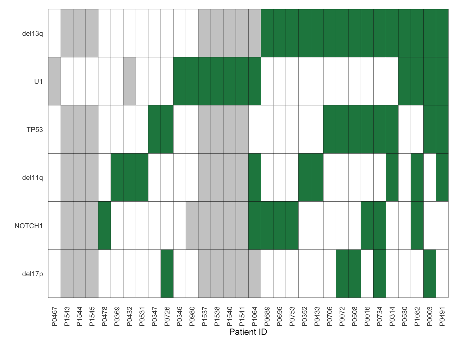 Please check if the annotations are correct
Differential protein expression using proDA
otherGenes <- colnames(geneMat)
resList <- lapply(otherGenes, function(n) {
  designMat <- geneMat[,n,drop=FALSE]
  designMat <- designMat[!is.na(designMat[[n]]),,drop=FALSE]
  testMat <- protMat[,rownames(designMat)]

  fit <- proDA(testMat, design = ~ .,
             col_data = designMat)

  contra <- n
  resTab <- proDA::test_diff(fit, contra) %>%
    dplyr::rename(id = name, logFC = diff, t=t_statistic,
                  P.Value = pval, adj.P.Val = adj_pval) %>%
    mutate(name = rowData(protCLL[id,])$hgnc_symbol) %>%
    select(name, id, logFC, t, P.Value, adj.P.Val) %>%
    arrange(P.Value) %>% mutate(Gene = n) %>%
    as_tibble()
  resTab
}) %>% bind_rows()
Save the results for re-using
save(resList, file = "../output/deResListBatch2.RData")Load the pre-calculated results (differential expression tests take long time.)
load("../output/deResListBatch2.RData")Summarise significant associations
Bar plot of number of significant associations (10% FDR)
plotTab <- resList %>% group_by(Gene) %>%
  summarise(nFDR.local = sum(adj.P.Val <= 0.1),
            nP = sum(P.Value < 0.01))
#Global adjusted P-values
plotTab <- arrange(plotTab, desc(nFDR.local)) %>% mutate(Gene = factor(Gene, levels = Gene))
ggplot(plotTab, aes(x=Gene, y = nFDR.local)) + geom_bar(stat="identity",fill=colList[2]) +
geom_text(aes(label = paste0("n=", nFDR.local)),vjust=-1,col=colList[1]) + ylim(0,40) +
theme_half + theme(axis.text.x = element_text(angle = 90, hjust=1, vjust=0.5)) +
ylab("Number of associations\n(10% FDR)") + xlab("")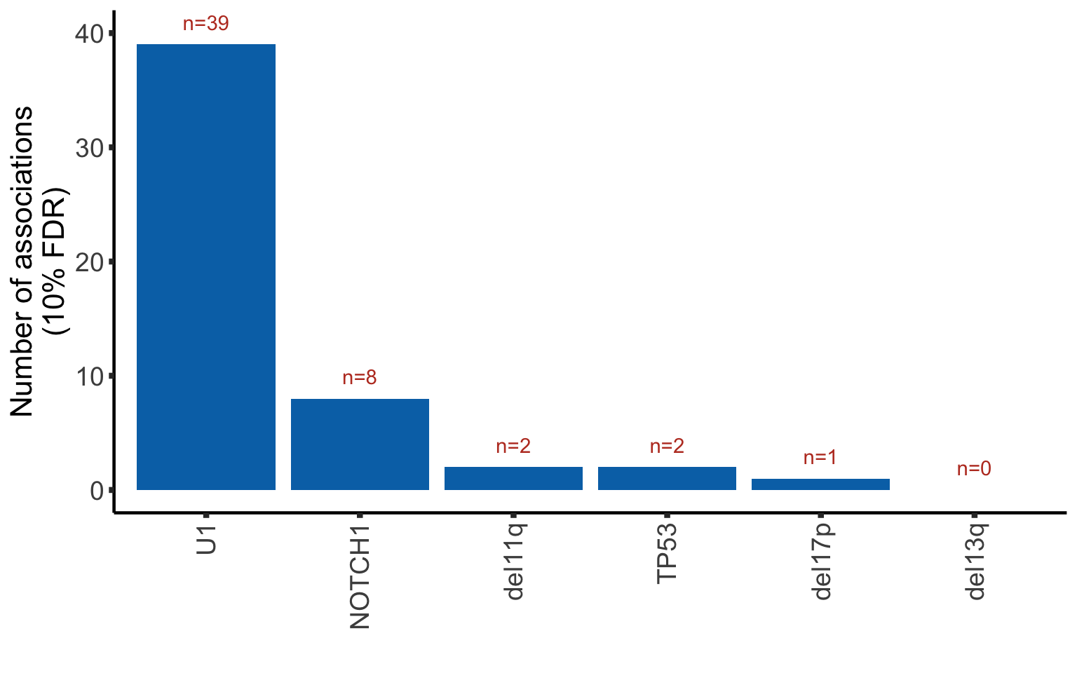
Bar plot of number of raw P-value < 0.01
plotTab <- arrange(plotTab, desc(nP)) %>% mutate(Gene = factor(Gene, levels = Gene))
ggplot(plotTab, aes(x=Gene, y = nP)) + geom_bar(stat="identity",fill=colList[2]) +
  geom_text(aes(label = paste0("n=", nP)),vjust=-1,col=colList[1]) + ylim(0,100) +
  theme_half + theme(axis.text.x = element_text(angle = 90, hjust=1, vjust=0.5)) +
  ylab("Number of associations\n(nominal P-value < 0.01)") + xlab("")
Table of all significant associations (P< 0.01)
resList.sig <- filter(resList, P.Value < 0.01) %>%
  select(name, Gene, logFC, P.Value, adj.P.Val,id) %>%
  arrange(P.Value)
resList.sig %>%
  mutate_if(is.numeric, formatC, digits=2) %>%
  DT::datatable()
Focused on U1 mutations
Heatmap of associated proteins (10% FDR)
resSub <- filter(resList, Gene == "U1", adj.P.Val < 0.1)
protMat <- assays(protCLL)[["QRILC"]][resSub$id,]
colAnno <- data.frame(row.names = colnames(protMat),
                      U1 = factor(geneMat[colnames(protMat),]$U1),
                      site = protCLL$site)

pheatmap::pheatmap(protMat, annotation_col = colAnno, scale = "row",
                   clustering_method = "ward.D2",
                   color = colorRampPalette(c(colList[2],"white",colList[1]))(100),
                   breaks = seq(-5,5, length.out = 101),
                   show_rownames = TRUE, show_colnames = TRUE,
                   labels_row = resSub$name,
                   treeheight_row = 0)
Pathway enrichment
Barplot of enriched pathways
gmts = list(H= "../data/gmts/h.all.v6.2.symbols.gmt",
            KEGG = "../data/gmts/c2.cp.kegg.v6.2.symbols.gmt")
protMat <-assays(protCLL)[["QRILC"]] #without imputation
designMat <- model.matrix(~U1, geneMat)
protMat <- protMat[,rownames(designMat) ]
enRes <-  runCamera(protMat, designMat, gmts$H,
                    id = rowData(protCLL)[rownames(protMat),]$hgnc_symbol,
                    contrast  = "U1",
            removePrefix = "HALLMARK_", pCut = 0.1, ifFDR = TRUE, plotTitle = "HALLMARK")
p1 <- enRes$enrichPlot

enRes <-  runCamera(protMat, designMat, gmts$KEGG,
                    id = rowData(protCLL)[rownames(protMat),]$hgnc_symbol,
                    contrast  = "U1",
            removePrefix = "KEGG_", pCut = 0.1, ifFDR = TRUE, plotTitle = "KEGG")
p2 <- enRes$enrichPlot

cowplot::plot_grid(p1,p2, ncol=1, align = "hv", axis = "lr", rel_heights = c(1,4))
Compare RNA and protein fold changes
Identify RNAs associated with U1 mutations
RNAseq samples are subsetted to the samples with proteomic data
ddsSub <- dds[rownames(dds) %in% rowData(protCLL)$ensembl_gene_id,dds$PatID %in% rownames(geneMat)]
ddsSub$U1 <- geneMat[match(ddsSub$PatID, rownames(geneMat)),]$U1
ddsSub <- ddsSub[,!is.na(ddsSub$U1)]
How many RNA seq samples with U1 information?
table(ddsSub$U1)
 0  1
16  4
DEseq
design(ddsSub) <- ~U1
deRes <- DESeq(ddsSub)
rnaRes <- results(deRes, tidy = TRUE) %>%
  select(row, log2FoldChange, pvalue, padj) %>%
  dplyr::rename(enID=row, logFC.rna = log2FoldChange, P.Value.rna = pvalue, adj.P.Val.rna =padj)
compareTab <- resList %>% filter(Gene == "U1") %>%
mutate(enID = rowData(protCLL[id,])$ensembl_gene_id) %>%
left_join(rnaRes, by = "enID") %>%
mutate(logFC.rna = ifelse(is.na(logFC.rna),0,logFC.rna),
P.Value.rna = ifelse(is.na(P.Value.rna),1,P.Value.rna)) %>%
mutate(significant = case_when(
adj.P.Val < 0.1 & adj.P.Val.rna < 0.1 ~ "both",
adj.P.Val < 0.1 & adj.P.Val.rna > 0.1 ~ "only protein",
adj.P.Val > 0.1 & adj.P.Val.rna < 0.1 ~ "only RNA",
TRUE ~"none"
)) %>%
filter(significant != "none")Plot
Only gene that show associations with either RNA or proteins at 10% FDR are shown
ggplot(compareTab, aes(x=logFC, y=logFC.rna, col = significant)) +
  geom_point() +
  theme_bw() +
  ggrepel::geom_text_repel(aes(label=name)) +
  xlab("logFC (Protein)") + ylab("logFC (RNA)")
Focused on TP53 mutations
Heatmap of associated proteins (P value < 0.01)
Only two proteins passed FDR < 0.1
resSub <- filter(resList, Gene == "TP53", P.Value < 0.01)
protMat <- assays(protCLL)[["QRILC"]][resSub$id,]
colAnno <- data.frame(row.names = colnames(protMat),
                      TP53 = factor(geneMat[colnames(protMat),]$TP53),
                      site = protCLL$site)

pheatmap::pheatmap(protMat, annotation_col = colAnno, scale = "row",
                   clustering_method = "ward.D2",
                   color = colorRampPalette(c(colList[2],"white",colList[1]))(100),
                   breaks = seq(-5,5, length.out = 101),
                   show_rownames = TRUE, show_colnames = TRUE,
                   labels_row = resSub$name,
                   treeheight_row = 0)
Pathway enrichment
Barplot of enriched pathways
gmts = list(H= "../data/gmts/h.all.v6.2.symbols.gmt",
            KEGG = "../data/gmts/c2.cp.kegg.v6.2.symbols.gmt")
protMat <-assays(protCLL)[["QRILC"]] #without imputation
designMat <- model.matrix(~TP53, geneMat)
protMat <- protMat[,rownames(designMat) ]
enRes <-  runCamera(protMat, designMat, gmts$H,
                    id = rowData(protCLL)[rownames(protMat),]$hgnc_symbol,
                    contrast  = "TP53",
            removePrefix = "HALLMARK_", pCut = 0.1, ifFDR = TRUE, plotTitle = "HALLMARK")
p1 <- enRes$enrichPlot

enRes <-  runCamera(protMat, designMat, gmts$KEGG,
                    id = rowData(protCLL)[rownames(protMat),]$hgnc_symbol,
                    contrast  = "TP53",
            removePrefix = "KEGG_", pCut = 0.1, ifFDR = TRUE, plotTitle = "KEGG")
p2 <- enRes$enrichPlot

cowplot::plot_grid(p1,p2, ncol=1, align = "hv", axis = "lr", rel_heights = c(1,4))
Compare RNA and protein fold changes
Identify RNAs associated with TP53 mutations
RNAseq samples are subsetted to the samples with proteomic data
ddsSub <- dds[rownames(dds) %in% rowData(protCLL)$ensembl_gene_id,dds$PatID %in% rownames(geneMat)]
ddsSub$TP53 <- geneMat[match(ddsSub$PatID, rownames(geneMat)),]$TP53
ddsSub <- ddsSub[,!is.na(ddsSub$TP53)]
How many RNA seq samples with TP53 information?
table(ddsSub$TP53)
 0  1
13  9
DEseq
design(ddsSub) <- ~TP53
deRes <- DESeq(ddsSub)
rnaRes <- results(deRes, tidy = TRUE) %>%
  select(row, log2FoldChange, pvalue, padj) %>%
  dplyr::rename(enID=row, logFC.rna = log2FoldChange, P.Value.rna = pvalue, adj.P.Val.rna =padj)
Here I use P.Value < 0.01 as cut-off, otherwise there are only two protein candiates
compareTab <- resList %>% filter(Gene == "TP53") %>%
  mutate(enID = rowData(protCLL[id,])$ensembl_gene_id) %>%
  left_join(rnaRes, by = "enID") %>%
  mutate(logFC.rna = ifelse(is.na(logFC.rna),0,logFC.rna),
         P.Value.rna = ifelse(is.na(P.Value.rna),1,P.Value.rna)) %>%
  mutate(significant = case_when(
    P.Value < 0.01 & P.Value.rna < 0.01 ~ "both",
    P.Value < 0.01 & P.Value.rna > 0.01 ~ "only protein",
    P.Value > 0.01 & P.Value.rna < 0.01 ~ "only RNA",
    TRUE ~"none"
  )) %>%
  filter(significant != "none")
Plot
Only gene that show associations with either RNA or proteins at 10% FDR are shown
ggplot(compareTab, aes(x=logFC, y=logFC.rna, col = significant)) +
  geom_point() +
  theme_bw() +
  ggrepel::geom_text_repel(aes(label=name)) +
  xlab("logFC (Protein)") + ylab("logFC (RNA)")
Focused on NOTCH1 mutations
Heatmap of associated proteins (P value < 0.01)
resSub <- filter(resList, Gene == "NOTCH1", P.Value < 0.01)
protMat <- assays(protCLL)[["QRILC"]][resSub$id,]
colAnno <- data.frame(row.names = colnames(protMat),
                      NOTCH1 = factor(geneMat[colnames(protMat),]$NOTCH1),
                      site = protCLL$site)

pheatmap::pheatmap(protMat, annotation_col = colAnno, scale = "row",
                   clustering_method = "ward.D2",
                   color = colorRampPalette(c(colList[2],"white",colList[1]))(100),
                   breaks = seq(-5,5, length.out = 101),
                   show_rownames = TRUE, show_colnames = TRUE,
                   labels_row = resSub$name,
                   treeheight_row = 0)
Pathway enrichment
Barplot of enriched pathways
gmts = list(H= "../data/gmts/h.all.v6.2.symbols.gmt",
            KEGG = "../data/gmts/c2.cp.kegg.v6.2.symbols.gmt")
protMat <-assays(protCLL)[["QRILC"]] #without imputation
designMat <- model.matrix(~NOTCH1, geneMat)
protMat <- protMat[,rownames(designMat) ]
enRes <-  runCamera(protMat, designMat, gmts$H,
                    id = rowData(protCLL)[rownames(protMat),]$hgnc_symbol,
                    contrast  = "NOTCH1",
            removePrefix = "HALLMARK_", pCut = 0.1, ifFDR = TRUE, plotTitle = "HALLMARK")
p1 <- enRes$enrichPlot

enRes <-  runCamera(protMat, designMat, gmts$KEGG,
                    id = rowData(protCLL)[rownames(protMat),]$hgnc_symbol,
                    contrast  = "NOTCH1",
            removePrefix = "KEGG_", pCut = 0.1, ifFDR = TRUE, plotTitle = "KEGG")
p2 <- enRes$enrichPlot

cowplot::plot_grid(p1,p2, ncol=1, align = "hv", axis = "lr", rel_heights = c(1,4))
Compare RNA and protein fold changes
Identify RNAs associated with NOTCH1 mutations
RNAseq samples are subsetted to the samples with proteomic data
ddsSub <- dds[rownames(dds) %in% rowData(protCLL)$ensembl_gene_id,dds$PatID %in% rownames(geneMat)]
ddsSub$NOTCH1 <- geneMat[match(ddsSub$PatID, rownames(geneMat)),]$NOTCH1
ddsSub <- ddsSub[,!is.na(ddsSub$NOTCH1)]
How many RNA seq samples with NOTCH1 information?
table(ddsSub$NOTCH1)
 0  1
14  7
DEseq
design(ddsSub) <- ~NOTCH1
deRes <- DESeq(ddsSub)
rnaRes <- results(deRes, tidy = TRUE) %>%
  select(row, log2FoldChange, pvalue, padj) %>%
  dplyr::rename(enID=row, logFC.rna = log2FoldChange, P.Value.rna = pvalue, adj.P.Val.rna =padj)
Here I use P.Value < 0.01 as cut-off
compareTab <- resList %>% filter(Gene == "NOTCH1") %>%
  mutate(enID = rowData(protCLL[id,])$ensembl_gene_id) %>%
  left_join(rnaRes, by = "enID") %>%
  mutate(logFC.rna = ifelse(is.na(logFC.rna),0,logFC.rna),
         P.Value.rna = ifelse(is.na(P.Value.rna),1,P.Value.rna)) %>%
  mutate(significant = case_when(
    P.Value < 0.01 & P.Value.rna < 0.01 ~ "both",
    P.Value < 0.01 & P.Value.rna > 0.01 ~ "only protein",
    P.Value > 0.01 & P.Value.rna < 0.01 ~ "only RNA",
    TRUE ~"none"
  )) %>%
  filter(significant != "none")
Plot
Only gene that show associations with either RNA or proteins at 10% FDR are shown
ggplot(compareTab, aes(x=logFC, y=logFC.rna, col = significant)) +
  geom_point() +
  theme_bw() +
  ggrepel::geom_text_repel(aes(label=name)) +
  xlab("logFC (Protein)") + ylab("logFC (RNA)")
sessionInfo()R version 3.6.0 (2019-04-26)
Platform: x86_64-apple-darwin15.6.0 (64-bit)
Running under: macOS 10.15.7
Matrix products: default
BLAS: /Library/Frameworks/R.framework/Versions/3.6/Resources/lib/libRblas.0.dylib
LAPACK: /Library/Frameworks/R.framework/Versions/3.6/Resources/lib/libRlapack.dylib
locale:
[1] en_US.UTF-8/en_US.UTF-8/en_US.UTF-8/C/en_US.UTF-8/en_US.UTF-8
attached base packages:
[1] parallel stats4 stats graphics grDevices utils datasets
[8] methods base
other attached packages:
[1] latex2exp_0.4.0 forcats_0.5.0
[3] stringr_1.4.0 dplyr_1.0.0
[5] purrr_0.3.4 readr_1.3.1
[7] tidyr_1.1.0 tibble_3.0.3
[9] ggplot2_3.3.2 tidyverse_1.3.0
[11] IHW_1.14.0 proDA_1.1.2
[13] DESeq2_1.26.0 SummarizedExperiment_1.16.1
[15] DelayedArray_0.12.3 BiocParallel_1.20.1
[17] matrixStats_0.56.0 Biobase_2.46.0
[19] GenomicRanges_1.38.0 GenomeInfoDb_1.22.1
[21] IRanges_2.20.2 S4Vectors_0.24.4
[23] BiocGenerics_0.32.0 limma_3.42.2
loaded via a namespace (and not attached):
[1] readxl_1.3.1 backports_1.1.8 fastmatch_1.1-0
[4] Hmisc_4.4-0 workflowr_1.6.2 igraph_1.2.5
[7] shinydashboard_0.7.1 splines_3.6.0 crosstalk_1.1.0.1
[10] lpsymphony_1.14.0 digest_0.6.25 htmltools_0.5.0
[13] gdata_2.18.0 fansi_0.4.1 magrittr_1.5
[16] checkmate_2.0.0 memoise_1.1.0 cluster_2.1.0
[19] annotate_1.64.0 modelr_0.1.8 piano_2.2.0
[22] jpeg_0.1-8.1 colorspace_1.4-1 ggrepel_0.8.2
[25] blob_1.2.1 rvest_0.3.5 haven_2.3.1
[28] xfun_0.15 crayon_1.3.4 RCurl_1.98-1.2
[31] jsonlite_1.7.0 genefilter_1.68.0 survival_3.2-3
[34] glue_1.4.1 gtable_0.3.0 zlibbioc_1.32.0
[37] XVector_0.26.0 scales_1.1.1 pheatmap_1.0.12
[40] DBI_1.1.0 relations_0.6-9 Rcpp_1.0.5
[43] xtable_1.8-4 htmlTable_2.0.1 foreign_0.8-71
[46] bit_4.0.4 Formula_1.2-3 DT_0.14
[49] htmlwidgets_1.5.1 httr_1.4.1 fgsea_1.12.0
[52] gplots_3.0.4 RColorBrewer_1.1-2 acepack_1.4.1
[55] ellipsis_0.3.1 pkgconfig_2.0.3 XML_3.98-1.20
[58] farver_2.0.3 nnet_7.3-14 dbplyr_1.4.4
[61] locfit_1.5-9.4 tidyselect_1.1.0 labeling_0.3
[64] rlang_0.4.7 later_1.1.0.1 AnnotationDbi_1.48.0
[67] visNetwork_2.0.9 munsell_0.5.0 cellranger_1.1.0
[70] tools_3.6.0 cli_2.0.2 generics_0.0.2
[73] RSQLite_2.2.0 broom_0.7.0 fdrtool_1.2.15
[76] evaluate_0.14 fastmap_1.0.1 yaml_2.2.1
[79] knitr_1.29 bit64_0.9-7 fs_1.4.2
[82] caTools_1.18.0 mime_0.9 slam_0.1-47
[85] xml2_1.3.2 compiler_3.6.0 rstudioapi_0.11
[88] png_0.1-7 marray_1.64.0 reprex_0.3.0
[91] geneplotter_1.64.0 stringi_1.4.6 lattice_0.20-41
[94] Matrix_1.2-18 shinyjs_1.1 vctrs_0.3.1
[97] pillar_1.4.6 lifecycle_0.2.0 cowplot_1.0.0
[100] data.table_1.12.8 bitops_1.0-6 httpuv_1.5.4
[103] R6_2.4.1 latticeExtra_0.6-29 promises_1.1.1
[106] KernSmooth_2.23-17 gridExtra_2.3 gtools_3.8.2
[109] assertthat_0.2.1 rprojroot_1.3-2 withr_2.2.0
[112] GenomeInfoDbData_1.2.2 hms_0.5.3 grid_3.6.0
[115] rpart_4.1-15 rmarkdown_2.3 git2r_0.27.1
[118] sets_1.0-18 shiny_1.5.0 lubridate_1.7.9
[121] base64enc_0.1-3