Analysis of the correlations between RNA and protein expression
Junyan Lu
2021-02-16
Last updated: 2021-03-05
Checks: 6 1
Knit directory: CLLproteomics_batch13/analysis/
This reproducible R Markdown analysis was created with workflowr (version 1.6.2). The Checks tab describes the reproducibility checks that were applied when the results were created. The Past versions tab lists the development history.
The R Markdown is untracked by Git. To know which version of the R Markdown file created these results, you'll want to first commit it to the Git repo. If you're still working on the analysis, you can ignore this warning. When you're finished, you can run wflow_publish to commit the R Markdown file and build the HTML.
Great job! The global environment was empty. Objects defined in the global environment can affect the analysis in your R Markdown file in unknown ways. For reproduciblity it's best to always run the code in an empty environment.
The command set.seed(20200227) was run prior to running the code in the R Markdown file. Setting a seed ensures that any results that rely on randomness, e.g. subsampling or permutations, are reproducible.
Great job! Recording the operating system, R version, and package versions is critical for reproducibility.
Nice! There were no cached chunks for this analysis, so you can be confident that you successfully produced the results during this run.
Great job! Using relative paths to the files within your workflowr project makes it easier to run your code on other machines.
Great! You are using Git for version control. Tracking code development and connecting the code version to the results is critical for reproducibility.
The results in this page were generated with repository version 3fb50c5. See the Past versions tab to see a history of the changes made to the R Markdown and HTML files.
Note that you need to be careful to ensure that all relevant files for the analysis have been committed to Git prior to generating the results (you can use wflow_publish or wflow_git_commit). workflowr only checks the R Markdown file, but you know if there are other scripts or data files that it depends on. Below is the status of the Git repository when the results were generated:
Ignored files:
    Ignored:    .DS_Store
    Ignored:    .Rhistory
    Ignored:    .Rproj.user/
    Ignored:    analysis/.DS_Store
    Ignored:    analysis/.Rhistory
    Ignored:    analysis/compareTreatment_cache/
    Ignored:    analysis/manuscript_S1_Overview_cache/
    Ignored:    analysis/manuscript_S3_trisomy12_cache/
    Ignored:    analysis/manuscript_S4_trisomy19_cache/
    Ignored:    analysis/manuscript_S5_IGHV_cache/
    Ignored:    analysis/manuscript_S6_del11q_cache/
    Ignored:    analysis/manuscript_S7_SF3B1_cache/
    Ignored:    analysis/manuscript_S8_drugResponse_Outcomes_cache/
    Ignored:    analysis/manuscript_S9_STAT2_cache/
    Ignored:    code/.DS_Store
    Ignored:    code/.Rhistory
    Ignored:    data/.DS_Store
    Ignored:    output/.DS_Store

Untracked files:
    Untracked:  analysis/.trisomy12_norm.pdf
    Untracked:  analysis/STAT2splicing.Rmd
    Untracked:  analysis/analysisBatch2.Rmd
    Untracked:  analysis/bufferAnalysis.Rmd
    Untracked:  analysis/compareTreatment.Rmd
    Untracked:  analysis/compare_batch1_3.Rmd
    Untracked:  analysis/complexAnalysis_overall.Rmd
    Untracked:  analysis/corumPairs.csv
    Untracked:  analysis/manuscript_S1_Overview.Rmd
    Untracked:  analysis/manuscript_S2_genomicAssociation.Rmd
    Untracked:  analysis/manuscript_S3_trisomy12.Rmd
    Untracked:  analysis/manuscript_S4_trisomy19.Rmd
    Untracked:  analysis/manuscript_S5_IGHV.Rmd
    Untracked:  analysis/manuscript_S6_del11q.Rmd
    Untracked:  analysis/manuscript_S7_SF3B1.Rmd
    Untracked:  analysis/manuscript_S8_drugResponse_Outcomes.Rmd
    Untracked:  analysis/manuscript_S9_STAT2.Rmd
    Untracked:  analysis/protRNACor_eachPat.pdf
    Untracked:  analysis/test.pdf
    Untracked:  code/utils.R
    Untracked:  data/Fig1A.png
    Untracked:  data/allComplexes.txt
    Untracked:  data/exprCNV.RData
    Untracked:  data/gmts/
    Untracked:  data/proteins_in_complexes
    Untracked:  data/proteomic_LUMOS_batch13.RData
    Untracked:  output/MSH6_splicing.svg
    Untracked:  output/SUGP1_splicing.svg
    Untracked:  output/deResList.RData
    Untracked:  output/deResListBatch2.RData
    Untracked:  output/deResListRNA.RData
    Untracked:  output/deResList_timsTOF.RData
    Untracked:  output/dxdCLL.RData
    Untracked:  output/dxdCLL2.RData
    Untracked:  output/exprCNV.RData
    Untracked:  output/geneAnno.RData
    Untracked:  output/int_pairs.csv

Unstaged changes:
    Modified:   analysis/_site.yml
    Deleted:    analysis/analysisSF3B1.Rmd
    Deleted:    analysis/comparePlatforms.Rmd
    Deleted:    analysis/compareProteomicsRNAseq.Rmd
    Deleted:    analysis/correlateCLLPD.Rmd
    Deleted:    analysis/correlateGenomic.Rmd
    Deleted:    analysis/correlateGenomic_removePC.Rmd
    Deleted:    analysis/correlateMIR.Rmd
    Deleted:    analysis/correlateMethylationCluster.Rmd
    Modified:   analysis/index.Rmd
    Deleted:    analysis/predictOutcome.Rmd
    Deleted:    analysis/processProteomics_LUMOS.Rmd
    Deleted:    analysis/processProteomics_timsTOF.Rmd
    Deleted:    analysis/qualityControl_LUMOS.Rmd
    Deleted:    analysis/qualityControl_timsTOF.Rmd
Note that any generated files, e.g. HTML, png, CSS, etc., are not included in this status report because it is ok for generated content to have uncommitted changes.
There are no past versions. Publish this analysis with wflow_publish() to start tracking its development.
Calculate protein-RNA correlations
Process both datasets
colnames(dds) <- dds$PatID
dds <- estimateSizeFactors(dds)
sampleOverlap <- intersect(colnames(protCLL), colnames(dds))
geneOverlap <- intersect(rowData(protCLL)$ensembl_gene_id, rownames(dds))
ddsSub <- dds[geneOverlap, sampleOverlap]
protSub <- protCLL[match(geneOverlap, rowData(protCLL)$ensembl_gene_id), sampleOverlap]

#how many gene don't have RNA expression at all?
noExp <- rowSums(counts(ddsSub)) == 0

#remove those genes in both datasets
ddsSub <- ddsSub[!noExp,]
protSub <- protSub[!noExp,]

#remove proteins with duplicated identifiers
protSub <- protSub[!duplicated(rowData(protSub)$name)]

geneOverlap <- intersect(rowData(protSub)$ensembl_gene_id, rownames(ddsSub))

ddsSub.vst <- varianceStabilizingTransformation(ddsSub)
Calculate correlations between protein abundance and RNA expression
rnaMat <- assay(ddsSub.vst)
proMat <- assays(protSub)[["QRILC_combat"]]
rownames(proMat) <- rowData(protSub)$ensembl_gene_id

corTab <- lapply(geneOverlap, function(n) {
  rna <- rnaMat[n,]
  pro.raw <- proMat[n,]
  res.raw <- cor.test(rna, pro.raw, use = "pairwise.complete.obs")
  tibble(id = n,
         p = res.raw$p.value,
         coef = res.raw$estimate)
}) %>% bind_rows() %>%
  arrange(desc(coef)) %>% mutate(p.adj = p.adjust(p, method = "BH"),
                                 symbol = rowData(dds[id,])$symbol,
                                 chr = rowData(dds[id,])$chromosome)
Plot the distribution of correlation coefficient
ggplot(corTab, aes(x=coef)) + geom_histogram(position = "identity", col = "grey50", alpha =0.3, bins =100) +
geom_vline(xintercept = 0, col = "red", linetype = "dashed") +
xlab("Pearson's correlation coefficient") 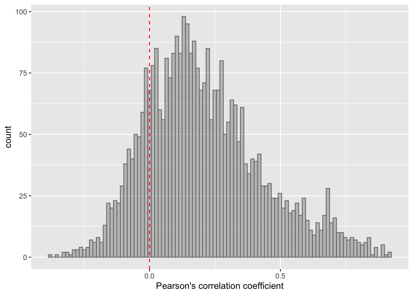 Most of the correlations are positive, which is reasonable.
ggplot(filter(corTab,!is.na(chr)), aes(x=coef)) + geom_histogram(position = "identity", col = "grey50", alpha =0.3, bins =100) +
geom_vline(xintercept = 0, col = "red", linetype = "dashed") + facet_wrap(~chr,ncol=3) +
xlab("Pearson's correlation coefficient") 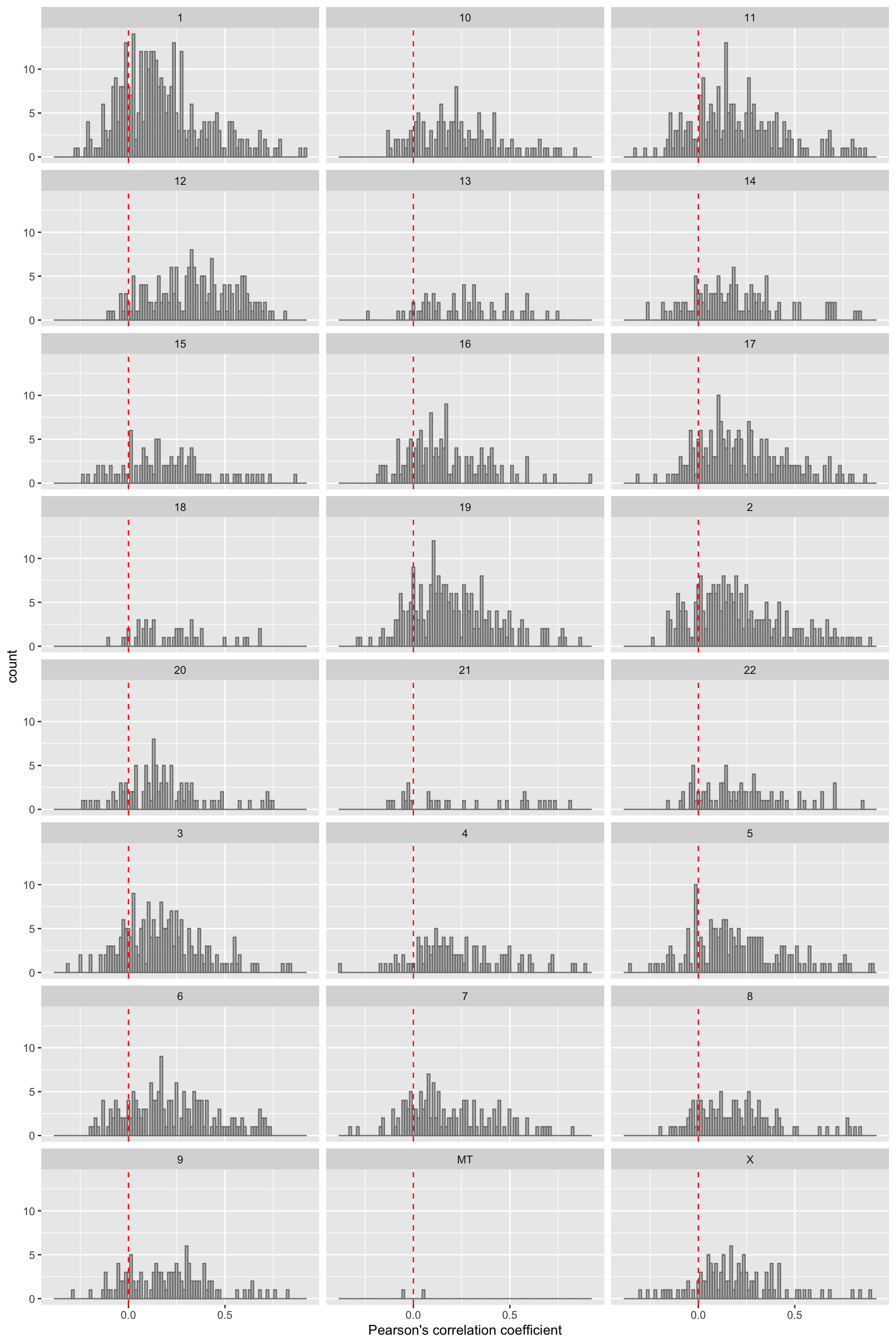 Similar trend can be observed for each chromosome.
For proteins in complex and not in complex
int_pairs = read_csv2("../output/int_pairs.csv")

sourceTab <- int_pairs %>%
  dplyr::select(ProtA, ProtB, database) %>% gather(key = "prot", value = "id", -database) %>%
  distinct(database, id) %>%
  mutate(id = rowData(protCLL)$ensembl_gene_id[match(id, rownames(protCLL))])

comGene <- sourceTab$id
corTab <- corTab %>% mutate(inComplex = ifelse(id %in% comGene, "yes","no")) %>%
mutate(database = sourceTab[match(id, sourceTab$id),]$database)
ggplot(corTab, aes(x=coef, fill = inComplex, y=..density..)) + geom_histogram(position = "identity", col = "grey50", alpha =0.3, bins =100) +
geom_vline(xintercept = 0, col = "red", linetype = "dashed") +
xlab("Pearson's correlation coefficient") 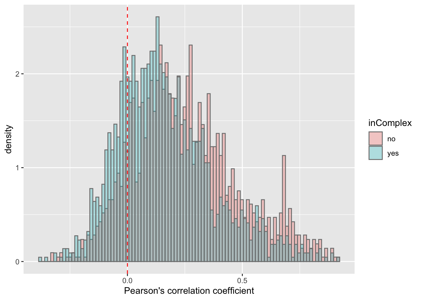 There's a slight trend that proteins not in complex tend to have higher protein-RNA expression correlations, which is reasonable, as proteins form complexes may be more regulated by buffering effect.
T-test
t.test(coef~inComplex, corTab, var.equal = TRUE )
    Two Sample t-test

data:  coef by inComplex
t = 11.823, df = 3289, p-value < 2.2e-16
alternative hypothesis: true difference in means is not equal to 0
95 percent confidence interval:
 0.07544552 0.10544501
sample estimates:
 mean in group no mean in group yes
        0.2536236         0.1631783
ggplot(corTab, aes(x=inComplex, y = coef))+geom_boxplot(aes(fill = inComplex)) + geom_point() +
theme_bw()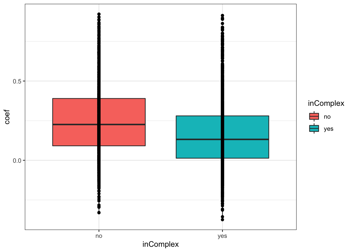
pList <- lapply(na.omit(unique(corTab$database)), function(n) {
plotTab <- filter(corTab, database %in% c(n,NA)) %>%
mutate(database = ifelse(is.na(database),"none",database)) %>%
mutate(database = factor(database, levels = c("none",n)))
p1 <- ggplot(plotTab, aes(x=coef, fill = database, y=..density..)) +
geom_histogram(position = "identity", col = "grey50", alpha =0.3, bins =100) +
geom_vline(xintercept = 0, col = "red", linetype = "dashed") +
xlab("Pearson's correlation coefficient")
p2 <- ggplot(plotTab, aes(x=database, fill = database, y=coef)) +
geom_boxplot() + geom_point() +
ylab("Pearson's correlation coefficient")
cowplot::plot_grid(p1,p2)
})
cowplot::plot_grid(plotlist = pList, ncol=1)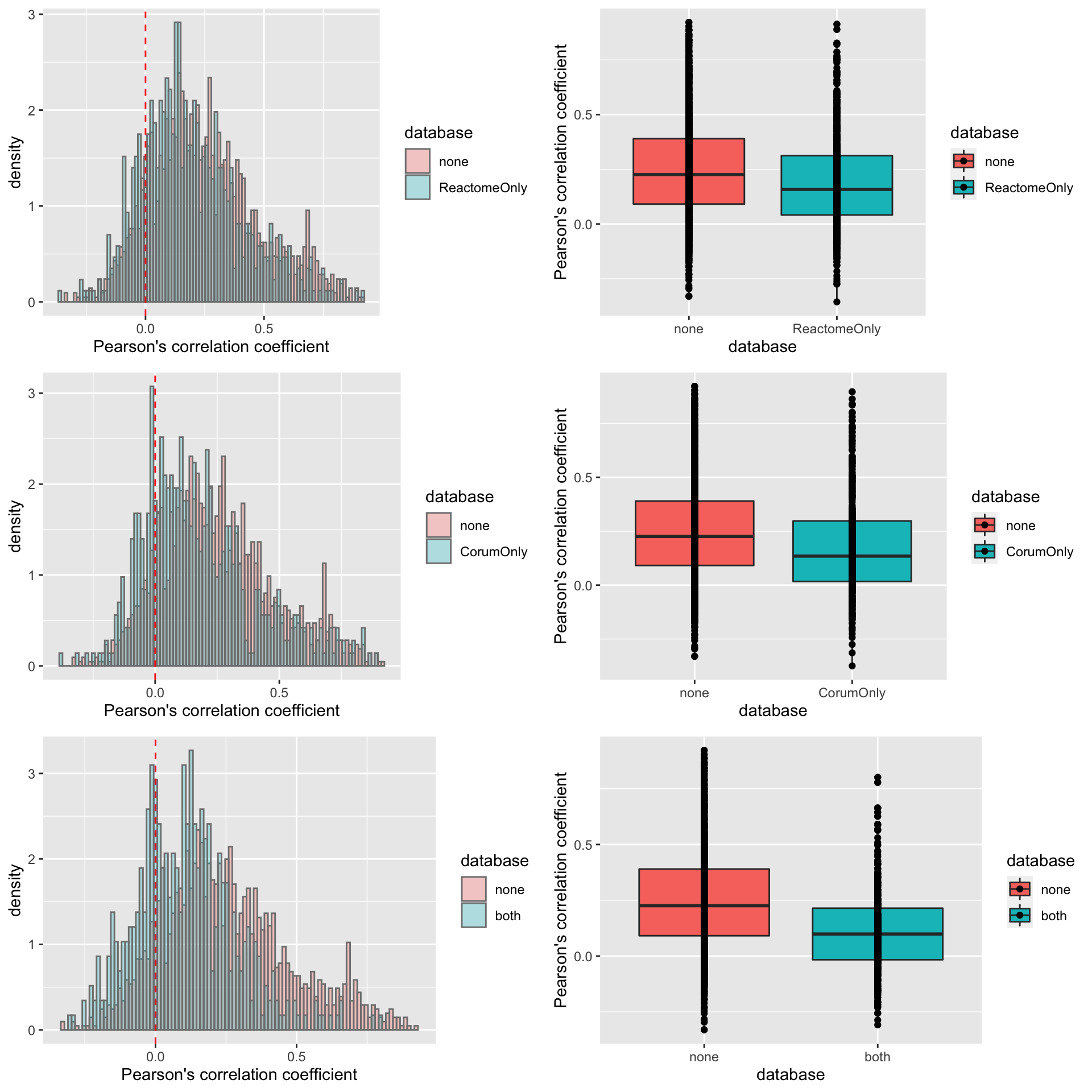 It seems the difference of correlations coefficient between proteins in complex and not in complex is stronger if we use more stringent criteria for proteins in complexes (annotated as in complexes by both Corum and reactome).
Per chromosome
ggplot(filter(corTab,!is.na(chr)), aes(x=coef,y=..density.., fill =inComplex)) + geom_histogram(position = "identity", col = "grey50", alpha =0.3, bins =100) +
  geom_vline(xintercept = 0, col = "red", linetype = "dashed") + facet_wrap(~chr,ncol=3, scale = "free") +
xlab("Pearson's correlation coefficient") 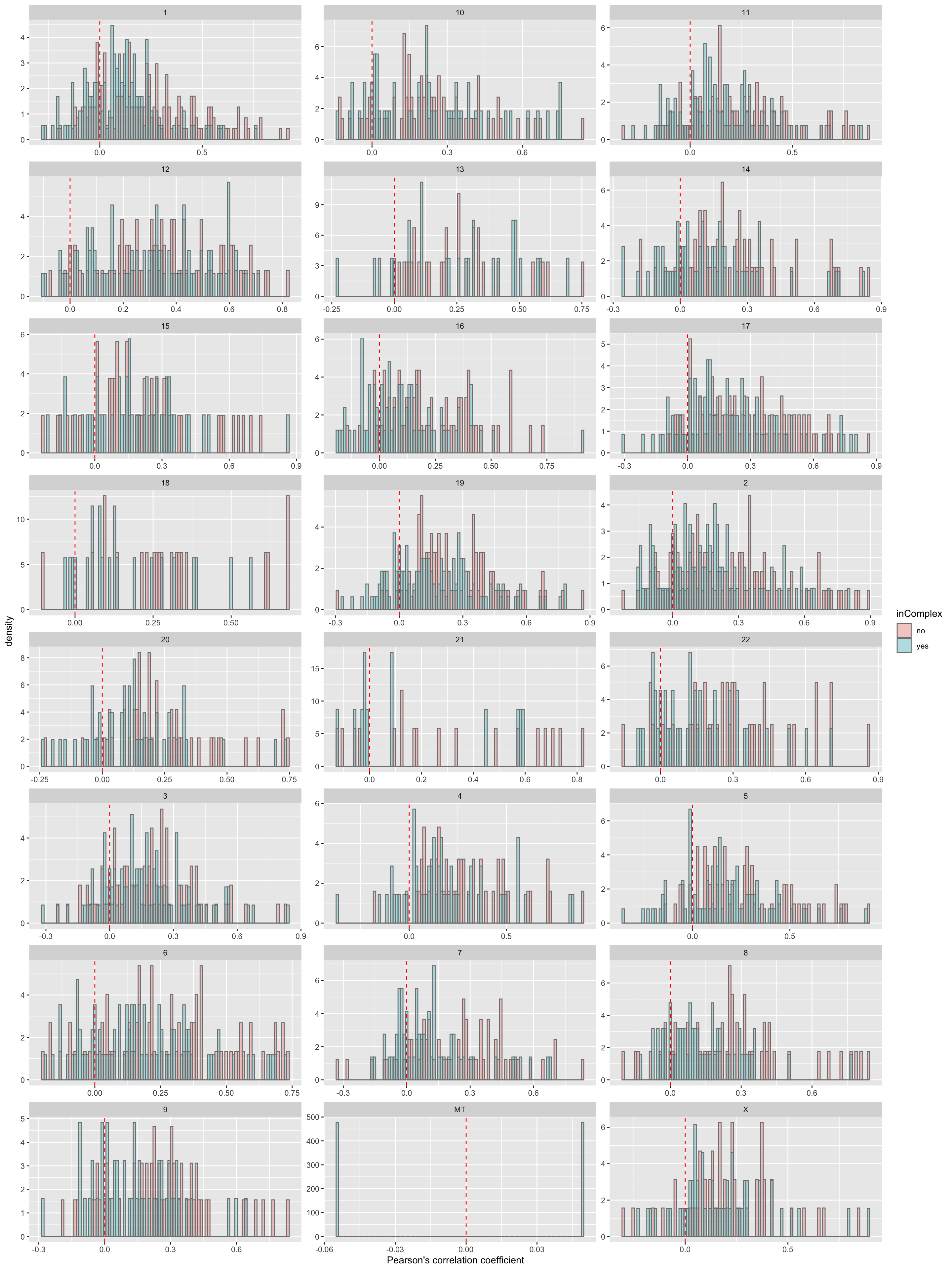
For proteins on chr12
plotTab <- filter(corTab, chr == "12")
ggplot(plotTab, aes(x=coef,y=..density.., fill =inComplex)) +
geom_histogram(position = "identity", col = "grey50", alpha =0.3, bins =100) +
geom_vline(xintercept = 0, col = "red", linetype = "dashed") +
xlab("Pearson's correlation coefficient") 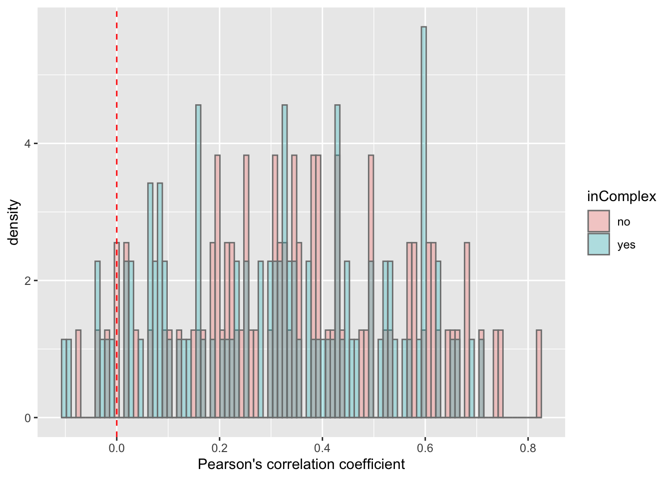 T-test
t.test(coef~inComplex, plotTab, var.equal = TRUE )
    Two Sample t-test

data:  coef by inComplex
t = 1.5986, df = 176, p-value = 0.1117
alternative hypothesis: true difference in means is not equal to 0
95 percent confidence interval:
 -0.01179482  0.11236151
sample estimates:
 mean in group no mean in group yes
        0.3556980         0.3054147
ggplot(plotTab, aes(x=inComplex, y = coef))+geom_boxplot(aes(fill = inComplex)) + geom_point() +
theme_bw()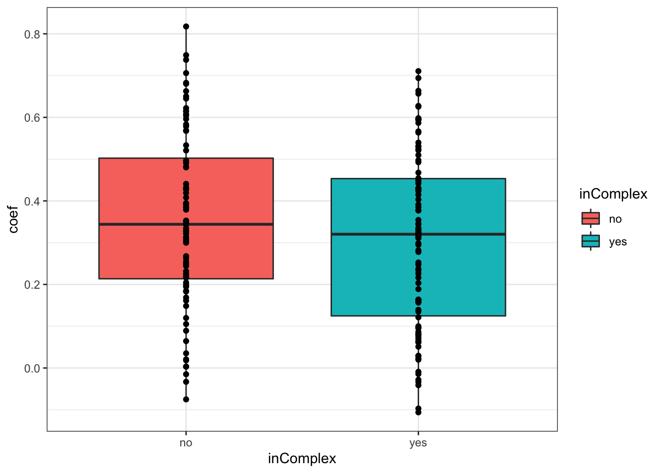
For proteins on chr19
plotTab <- filter(corTab, chr == "19")
ggplot(plotTab, aes(x=coef,y=..density.., fill =inComplex)) +
  geom_histogram(position = "identity", col = "grey50", alpha =0.3, bins =100) +
  geom_vline(xintercept = 0, col = "red", linetype = "dashed") +
xlab("Pearson's correlation coefficient") 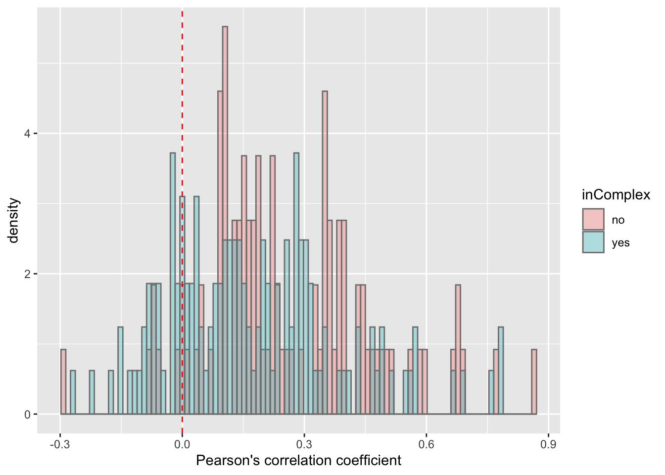
T-test
t.test(coef~inComplex, plotTab, var.equal = TRUE )
    Two Sample t-test

data:  coef by inComplex
t = 3.2206, df = 229, p-value = 0.001465
alternative hypothesis: true difference in means is not equal to 0
95 percent confidence interval:
 0.0350777 0.1456474
sample estimates:
 mean in group no mean in group yes
        0.2588620         0.1684995
ggplot(plotTab, aes(x=inComplex, y = coef))+geom_boxplot(aes(fill = inComplex)) + geom_point() +
theme_bw()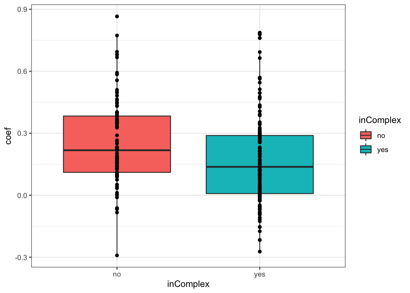
Protein-RNA correlation across proteins
load("../output/exprCNV.RData")overPat <- intersect(unique(allProtTab$patID), unique(allRnaTab$patID))
plotList <- lapply(overPat, function(pat) {
ttPro <- dplyr::filter(allProtTab, patID %in% pat) %>%
select(id, expr, ChromID)
ttRna <- dplyr::filter(allRnaTab, patID %in% pat) %>%
select(id, expr) %>% dplyr::rename(exprRna = expr)
ttComb <- left_join(ttRna, ttPro, by = "id") %>%
filter(!is.na(exprRna),!is.na(expr)) %>%
mutate(chr12 = ifelse(ChromID %in% "chr12", "yes","no"))
q <- ggplot(ttComb, aes(x=exprRna, y=expr, col = chr12)) + geom_point() +
ggtitle(pat) +
theme_bw()
q
})
makepdf(plotList, "protRNACor_eachPat.pdf", ncol=3, nrow=3, height = 12, width = 12)
sessionInfo()R version 3.6.0 (2019-04-26)
Platform: x86_64-apple-darwin15.6.0 (64-bit)
Running under: macOS 10.16
Matrix products: default
BLAS: /Library/Frameworks/R.framework/Versions/3.6/Resources/lib/libRblas.0.dylib
LAPACK: /Library/Frameworks/R.framework/Versions/3.6/Resources/lib/libRlapack.dylib
locale:
[1] en_US.UTF-8/en_US.UTF-8/en_US.UTF-8/C/en_US.UTF-8/en_US.UTF-8
attached base packages:
[1] parallel stats4 stats graphics grDevices utils datasets
[8] methods base
other attached packages:
[1] gridExtra_2.3 forcats_0.5.0
[3] stringr_1.4.0 dplyr_1.0.0
[5] purrr_0.3.4 readr_1.3.1
[7] tidyr_1.1.0 tibble_3.0.3
[9] ggplot2_3.3.2 tidyverse_1.3.0
[11] proDA_1.1.2 DESeq2_1.26.0
[13] SummarizedExperiment_1.16.1 DelayedArray_0.12.3
[15] BiocParallel_1.20.1 matrixStats_0.56.0
[17] Biobase_2.46.0 GenomicRanges_1.38.0
[19] GenomeInfoDb_1.22.1 IRanges_2.20.2
[21] S4Vectors_0.24.4 BiocGenerics_0.32.0
[23] jyluMisc_0.1.5 limma_3.42.2
loaded via a namespace (and not attached):
[1] readxl_1.3.1 backports_1.1.8 Hmisc_4.4-0
[4] fastmatch_1.1-0 drc_3.0-1 workflowr_1.6.2
[7] igraph_1.2.5 shinydashboard_0.7.1 splines_3.6.0
[10] TH.data_1.0-10 digest_0.6.25 htmltools_0.5.0
[13] fansi_0.4.1 gdata_2.18.0 memoise_1.1.0
[16] magrittr_1.5 checkmate_2.0.0 cluster_2.1.0
[19] openxlsx_4.1.5 annotate_1.64.0 modelr_0.1.8
[22] sandwich_2.5-1 piano_2.2.0 jpeg_0.1-8.1
[25] colorspace_1.4-1 rvest_0.3.5 blob_1.2.1
[28] haven_2.3.1 xfun_0.15 crayon_1.3.4
[31] RCurl_1.98-1.2 jsonlite_1.7.0 genefilter_1.68.0
[34] survival_3.2-3 zoo_1.8-8 glue_1.4.1
[37] survminer_0.4.7 gtable_0.3.0 zlibbioc_1.32.0
[40] XVector_0.26.0 car_3.0-8 abind_1.4-5
[43] scales_1.1.1 mvtnorm_1.1-1 DBI_1.1.0
[46] relations_0.6-9 rstatix_0.6.0 Rcpp_1.0.5
[49] plotrix_3.7-8 xtable_1.8-4 htmlTable_2.0.1
[52] bit_4.0.4 foreign_0.8-71 km.ci_0.5-2
[55] Formula_1.2-3 DT_0.14 httr_1.4.1
[58] htmlwidgets_1.5.1 fgsea_1.12.0 gplots_3.0.4
[61] RColorBrewer_1.1-2 acepack_1.4.1 ellipsis_0.3.1
[64] farver_2.0.3 XML_3.98-1.20 pkgconfig_2.0.3
[67] dbplyr_1.4.4 nnet_7.3-14 locfit_1.5-9.4
[70] labeling_0.3 AnnotationDbi_1.48.0 tidyselect_1.1.0
[73] rlang_0.4.7 later_1.1.0.1 munsell_0.5.0
[76] cellranger_1.1.0 tools_3.6.0 visNetwork_2.0.9
[79] cli_2.0.2 RSQLite_2.2.0 generics_0.0.2
[82] broom_0.7.0 evaluate_0.14 fastmap_1.0.1
[85] yaml_2.2.1 bit64_0.9-7 knitr_1.29
[88] fs_1.4.2 zip_2.0.4 survMisc_0.5.5
[91] caTools_1.18.0 mime_0.9 slam_0.1-47
[94] xml2_1.3.2 compiler_3.6.0 rstudioapi_0.11
[97] curl_4.3 png_0.1-7 ggsignif_0.6.0
[100] marray_1.64.0 reprex_0.3.0 geneplotter_1.64.0
[103] stringi_1.4.6 lattice_0.20-41 Matrix_1.2-18
[106] shinyjs_1.1 KMsurv_0.1-5 vctrs_0.3.1
[109] pillar_1.4.6 lifecycle_0.2.0 data.table_1.12.8
[112] cowplot_1.0.0 bitops_1.0-6 httpuv_1.5.4
[115] R6_2.4.1 latticeExtra_0.6-29 promises_1.1.1
[118] KernSmooth_2.23-17 rio_0.5.16 codetools_0.2-16
[121] assertthat_0.2.1 MASS_7.3-51.6 gtools_3.8.2
[124] exactRankTests_0.8-31 rprojroot_1.3-2 withr_2.2.0
[127] multcomp_1.4-13 GenomeInfoDbData_1.2.2 hms_0.5.3
[130] grid_3.6.0 rpart_4.1-15 rmarkdown_2.3
[133] carData_3.0-4 git2r_0.27.1 maxstat_0.7-25
[136] ggpubr_0.4.0 sets_1.0-18 lubridate_1.7.9
[139] shiny_1.5.0 base64enc_0.1-3