Identify proteins differentially expressed between before and under treatment
Junyan Lu
2021-02-16
Last updated: 2021-02-16
Checks: 5 2
Knit directory: CLLproteomics_batch13/analysis/
This reproducible R Markdown analysis was created with workflowr (version 1.6.2). The Checks tab describes the reproducibility checks that were applied when the results were created. The Past versions tab lists the development history.
The R Markdown is untracked by Git. To know which version of the R Markdown file created these results, you'll want to first commit it to the Git repo. If you're still working on the analysis, you can ignore this warning. When you're finished, you can run wflow_publish to commit the R Markdown file and build the HTML.
Great job! The global environment was empty. Objects defined in the global environment can affect the analysis in your R Markdown file in unknown ways. For reproduciblity it's best to always run the code in an empty environment.
The command set.seed(20200227) was run prior to running the code in the R Markdown file. Setting a seed ensures that any results that rely on randomness, e.g. subsampling or permutations, are reproducible.
Great job! Recording the operating system, R version, and package versions is critical for reproducibility.
- unnamed-chunk-2
To ensure reproducibility of the results, delete the cache directory compareTreatment_cache and re-run the analysis. To have workflowr automatically delete the cache directory prior to building the file, set delete_cache = TRUE when running wflow_build() or wflow_publish().
Great job! Using relative paths to the files within your workflowr project makes it easier to run your code on other machines.
Great! You are using Git for version control. Tracking code development and connecting the code version to the results is critical for reproducibility.
The results in this page were generated with repository version 3fb50c5. See the Past versions tab to see a history of the changes made to the R Markdown and HTML files.
Note that you need to be careful to ensure that all relevant files for the analysis have been committed to Git prior to generating the results (you can use wflow_publish or wflow_git_commit). workflowr only checks the R Markdown file, but you know if there are other scripts or data files that it depends on. Below is the status of the Git repository when the results were generated:
Ignored files:
    Ignored:    .DS_Store
    Ignored:    .Rhistory
    Ignored:    .Rproj.user/
    Ignored:    analysis/.DS_Store
    Ignored:    analysis/.Rhistory
    Ignored:    analysis/compareTreatment_cache/
    Ignored:    analysis/manuscript_S1_Overview_cache/
    Ignored:    analysis/manuscript_S3_trisomy12_cache/
    Ignored:    analysis/manuscript_S4_trisomy19_cache/
    Ignored:    analysis/manuscript_S5_IGHV_cache/
    Ignored:    analysis/manuscript_S6_del11q_cache/
    Ignored:    analysis/manuscript_S7_SF3B1_cache/
    Ignored:    analysis/manuscript_S8_drugResponse_Outcomes_cache/
    Ignored:    analysis/manuscript_S9_STAT2_cache/
    Ignored:    code/.DS_Store
    Ignored:    code/.Rhistory
    Ignored:    data/.DS_Store
    Ignored:    output/.DS_Store

Untracked files:
    Untracked:  analysis/.trisomy12_norm.pdf
    Untracked:  analysis/compareTreatment.Rmd
    Untracked:  analysis/compare_batch1_3.Rmd
    Untracked:  analysis/complexAnalysis_overall.Rmd
    Untracked:  analysis/manuscript_S1_Overview.Rmd
    Untracked:  analysis/manuscript_S2_genomicAssociation.Rmd
    Untracked:  analysis/manuscript_S3_trisomy12.Rmd
    Untracked:  analysis/manuscript_S4_trisomy19.Rmd
    Untracked:  analysis/manuscript_S5_IGHV.Rmd
    Untracked:  analysis/manuscript_S6_del11q.Rmd
    Untracked:  analysis/manuscript_S7_SF3B1.Rmd
    Untracked:  analysis/manuscript_S8_drugResponse_Outcomes.Rmd
    Untracked:  analysis/manuscript_S9_STAT2.Rmd
    Untracked:  analysis/test.pdf
    Untracked:  code/utils.R
    Untracked:  data/Fig1A.png
    Untracked:  data/exprCNV.RData
    Untracked:  data/gmts/
    Untracked:  data/proteins_in_complexes
    Untracked:  data/proteomic_LUMOS_batch13.RData
    Untracked:  output/MSH6_splicing.svg
    Untracked:  output/SUGP1_splicing.svg
    Untracked:  output/deResList.RData
    Untracked:  output/deResList_timsTOF.RData
    Untracked:  output/dxdCLL.RData
    Untracked:  output/dxdCLL2.RData
    Untracked:  output/exprCNV.RData
    Untracked:  output/geneAnno.RData
    Untracked:  output/splicingResults.RData

Unstaged changes:
    Modified:   analysis/_site.yml
    Deleted:    analysis/analysisSF3B1.Rmd
    Deleted:    analysis/comparePlatforms.Rmd
    Deleted:    analysis/compareProteomicsRNAseq.Rmd
    Deleted:    analysis/correlateCLLPD.Rmd
    Deleted:    analysis/correlateGenomic.Rmd
    Deleted:    analysis/correlateGenomic_removePC.Rmd
    Deleted:    analysis/correlateMIR.Rmd
    Deleted:    analysis/correlateMethylationCluster.Rmd
    Modified:   analysis/index.Rmd
    Deleted:    analysis/predictOutcome.Rmd
    Deleted:    analysis/processProteomics_LUMOS.Rmd
    Deleted:    analysis/processProteomics_timsTOF.Rmd
    Deleted:    analysis/qualityControl_LUMOS.Rmd
    Deleted:    analysis/qualityControl_timsTOF.Rmd
Note that any generated files, e.g. HTML, png, CSS, etc., are not included in this status report because it is ok for generated content to have uncommitted changes.
There are no past versions. Publish this analysis with wflow_publish() to start tracking its development.
Load packages and datasets
Annotated samples before and after treatment
protSub <- protCLL[,str_detect(colnames(protCLL),"_")]
protSub$treat <- factor(ifelse(str_detect(colnames(protSub),"_1"),"before","after"),
                        levels = c("before","after"))
protSub$patID <- str_remove(colnames(protSub),"_.")
Detect differentially expressed proteins
protMat <- assays(protSub)[["count"]]
design <- model.matrix(~patID + treat, colData(protSub))
fit <- proDA(protMat, design = design)
resTab <- test_diff(fit, contrast = "treatafter") %>%
  mutate(symbol = rowData(protCLL[name,])$hgnc_symbol) %>%
  arrange(pval)
P-value histogram
hist(resTab$pval, breaks = 50)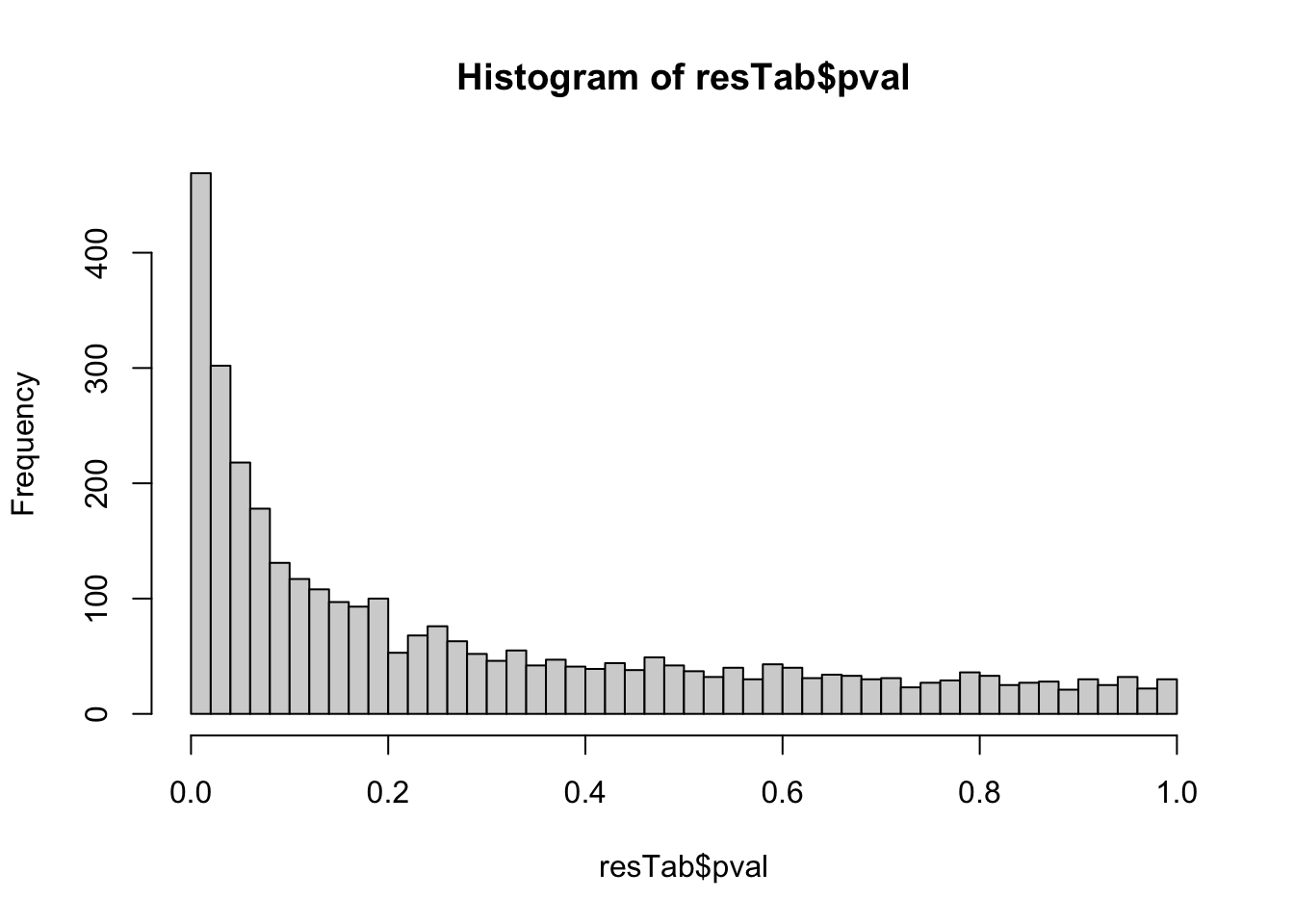
List of singificant proteins (P <=0.01)
resTab.sig <- filter(resTab, pval <=0.01)

resTab.sig %>% select(symbol, pval, adj_pval, diff, n_obs) %>%
  mutate_if(is.numeric, formatC, digits=2) %>%
DT::datatable()Boxplot of candidates
Plot top 9 most down regulated
proTab <- sumToTidy(protSub)
resTab.down <- filter(resTab.sig, diff < 0)
pList <- lapply(unique(resTab.down$symbol), function(nm) {
  plotTab <- filter(proTab, hgnc_symbol == nm)
  ggplot(plotTab, aes(x=treat, y=count)) +
    geom_boxplot() + geom_point(aes(col = treat)) +
    geom_line(aes(group = patID), linetype ="dashed",col = "grey50") +
    theme_bw() + ggtitle(nm) +
    theme(legend.position = "none",
          plot.title = element_text(hjust=0.5, face = "bold"))
})

cowplot::plot_grid(plotlist= pList[1:9], ncol=3)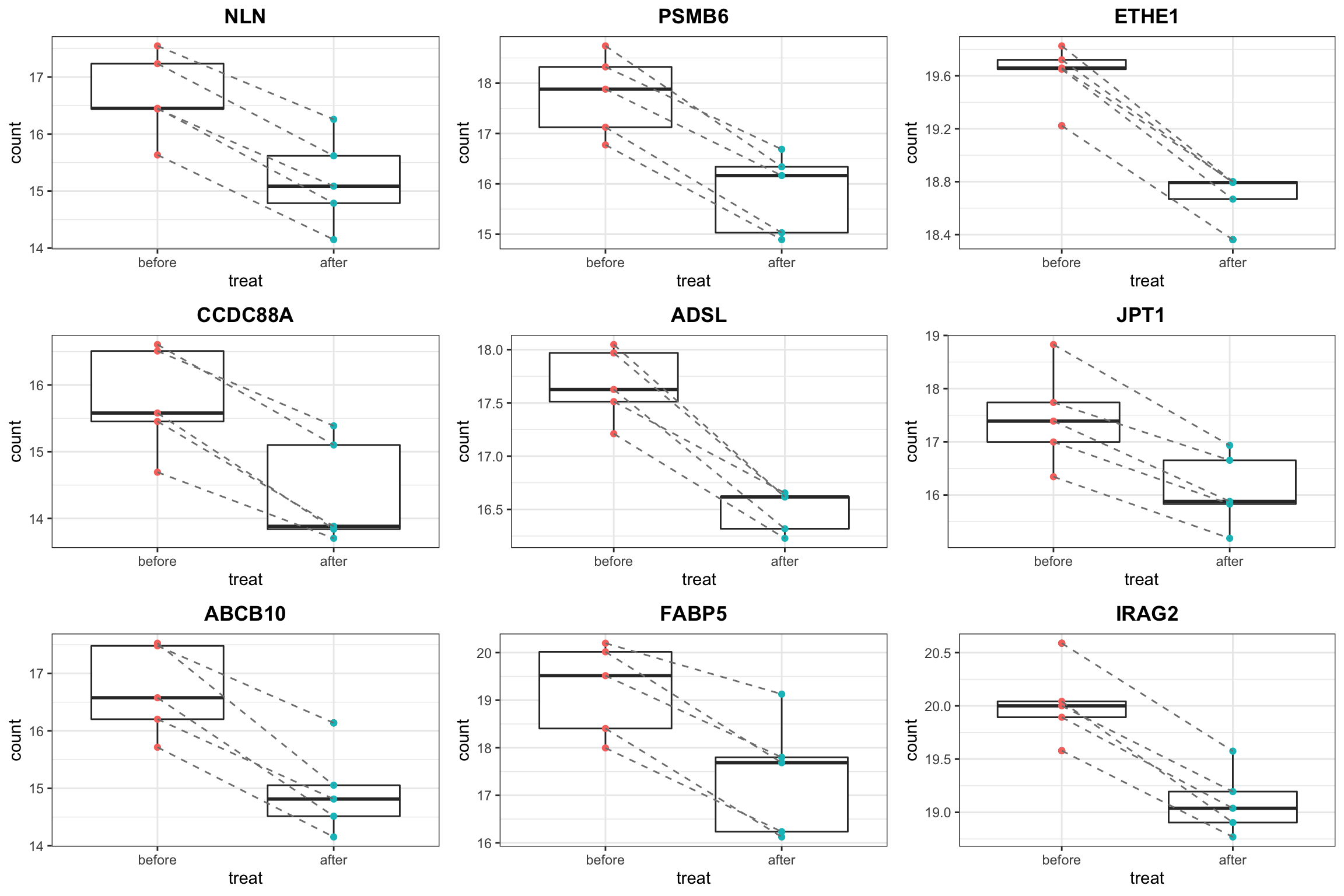
For all DE proteins (as pdf)
jyluMisc::makepdf(pList,"../public/treat_DOWN.pdf", ncol=3,nrow=3, height = 8, width = 12)Plot top 9 most up regulated
proTab <- sumToTidy(protSub)
resTab.up <- filter(resTab.sig, diff > 0)
pList <- lapply(unique(resTab.up$symbol)[1:9], function(nm) {
  plotTab <- filter(proTab, hgnc_symbol == nm)
  ggplot(plotTab, aes(x=treat, y=count)) +
    geom_boxplot() + geom_point(aes(col = treat)) +
    geom_line(aes(group = patID), linetype ="dashed",col = "grey50") +
    theme_bw() + ggtitle(nm) +
    theme(legend.position = "none",
          plot.title = element_text(hjust=0.5, face = "bold"))
})

cowplot::plot_grid(plotlist= pList, ncol=3)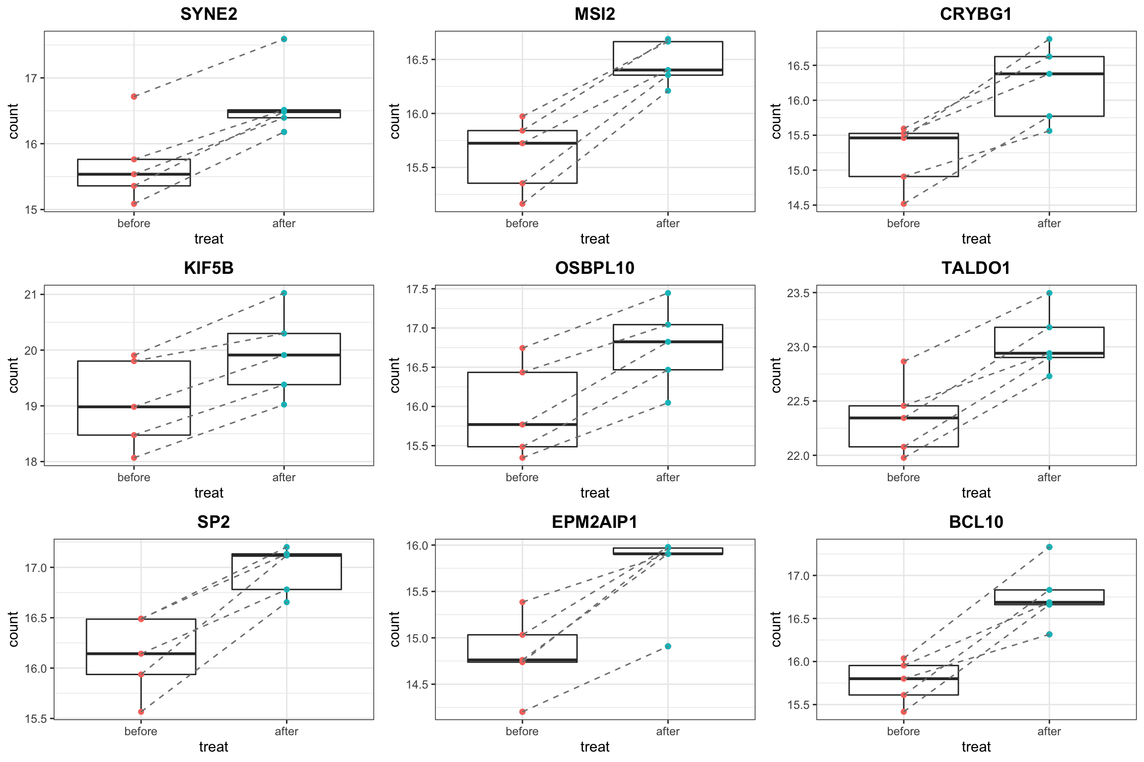
For all DE proteins (as pdf)
jyluMisc::makepdf(pList,"../public/treat_UP.pdf", ncol=3,nrow=3, height = 8, width = 12)Pathway enrichment
Enrichment using PAGE
Barplot of enriched pathways
gmts = list(H= "../data/gmts/h.all.v6.2.symbols.gmt",
KEGG = "../data/gmts/c2.cp.kegg.v6.2.symbols.gmt",
C6 = "../data/gmts/c6.all.v6.2.symbols.gmt")
inputTab <- resTab %>% filter(pval <= 0.05) %>%
distinct(symbol, .keep_all = TRUE) %>%
select(symbol, t_statistic) %>% data.frame() %>% column_to_rownames("symbol")
enRes <- list()
enRes[["HALLMARK"]] <- runGSEA(inputTab, gmts$H, "page")
enRes[["KEGG"]] <- runGSEA(inputTab, gmts$KEGG, "page")
enRes[["C6"]] <- runGSEA(inputTab, gmts$C6, "page")
p1 <- plotEnrichmentBar(enRes[[1]], pCut =0.1, ifFDR= TRUE, setName = "",
title = "HALLMARK gene set", removePrefix = "HALLMARK_", insideLegend=FALSE)
p2 <- plotEnrichmentBar(enRes[[2]], pCut =0.1, ifFDR= TRUE, setName = "",
title = "KEGG gene set", removePrefix = "KEGG_", insideLegend=FALSE)
p3 <- plotEnrichmentBar(enRes[[3]], pCut =0.1, ifFDR= TRUE, setName = "",
title = "C6: Oncogenetic signature", removePrefix = "KEGG_", insideLegend=FALSE)
treatEnrich <- cowplot::plot_grid(p1,p2, ncol=1, align = "hv", axis = "lr")
treatEnrich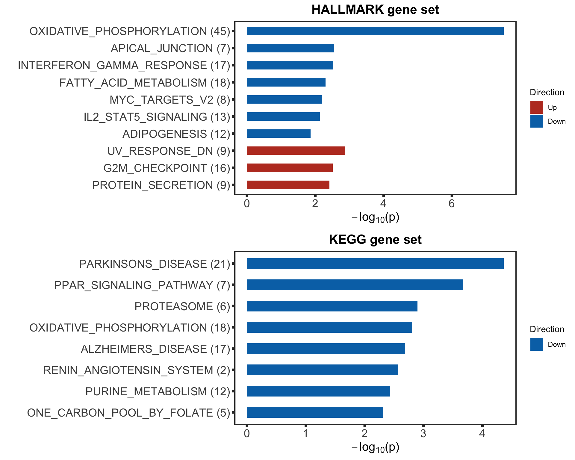 It looks like the treatment affected CLL proliferation related pathways, such as OXPHOS and MYC.
Enrichment using CAMERA
protMat <- assays(protSub)[["QRILC"]]
enRes <- runCamera(protMat, design, gmts$H,
id = rowData(protCLL)[rownames(protMat),]$hgnc_symbol,
contrast = "treatafter",
removePrefix = "HALLMARK_", pCut = 0.1, ifFDR = TRUE, plotTitle = "HALLMARK")
p1 <- enRes$enrichPlot
enRes <- runCamera(protMat, design, gmts$KEGG,
id = rowData(protCLL)[rownames(protMat),]$hgnc_symbol,
contrast = "treatafter",
removePrefix = "KEGG_", pCut = 0.1, ifFDR = TRUE, plotTitle = "KEGG")
p2 <- enRes$enrichPlot
cowplot::plot_grid(p1,p2, ncol=1, align = "hv", axis = "lr",
rel_heights = c(3,7))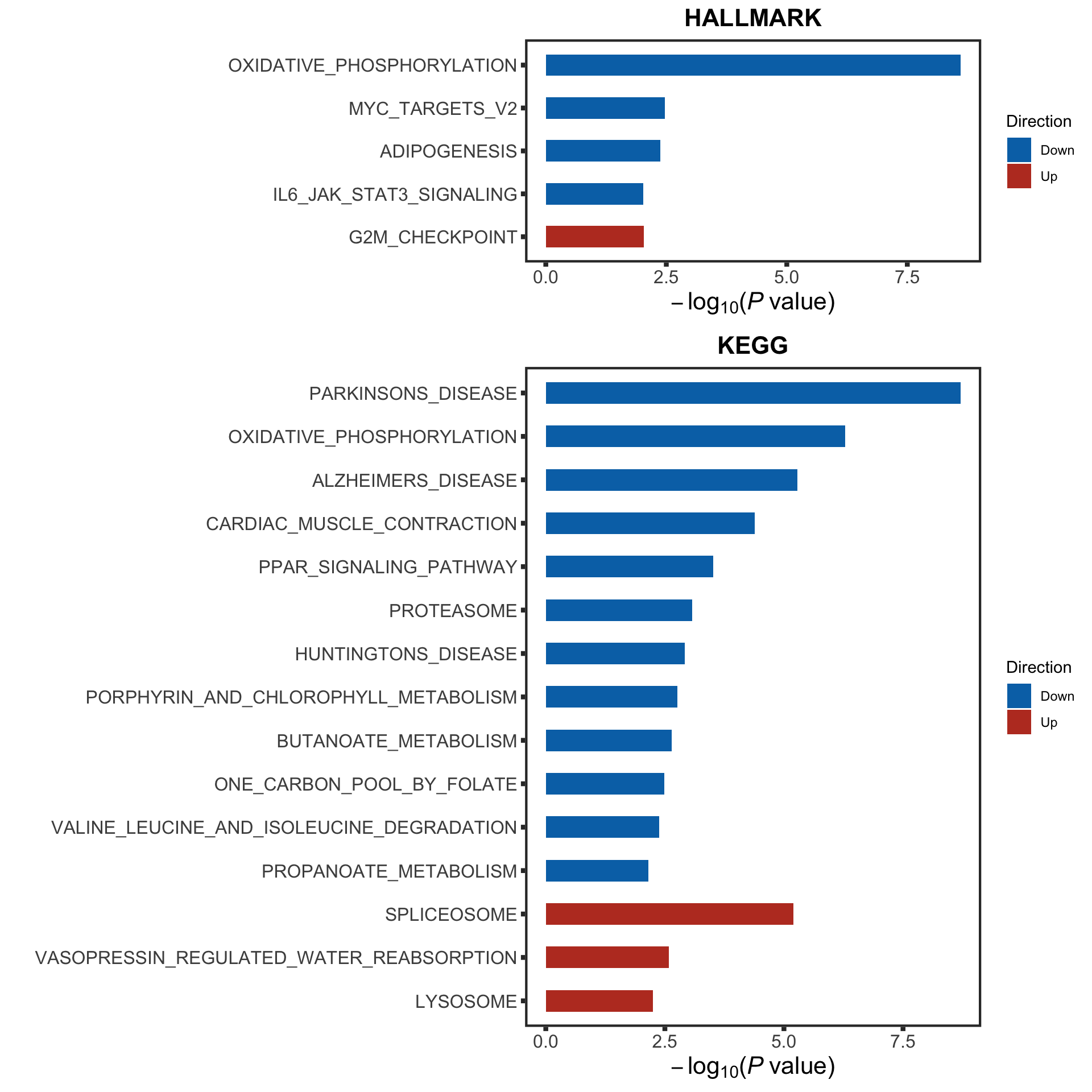 Similar results can be observed.
sessionInfo()R version 4.0.2 (2020-06-22)
Platform: x86_64-apple-darwin17.0 (64-bit)
Running under: macOS Catalina 10.15.7
Matrix products: default
BLAS: /Library/Frameworks/R.framework/Versions/4.0/Resources/lib/libRblas.dylib
LAPACK: /Library/Frameworks/R.framework/Versions/4.0/Resources/lib/libRlapack.dylib
locale:
[1] en_US.UTF-8/en_US.UTF-8/en_US.UTF-8/C/en_US.UTF-8/en_US.UTF-8
attached base packages:
[1] parallel stats4 stats graphics grDevices utils datasets
[8] methods base
other attached packages:
[1] piano_2.4.0 gridExtra_2.3
[3] latex2exp_0.4.0 forcats_0.5.0
[5] stringr_1.4.0 dplyr_1.0.0
[7] purrr_0.3.4 readr_1.3.1
[9] tidyr_1.1.0 tibble_3.0.2
[11] ggplot2_3.3.2 tidyverse_1.3.0
[13] SummarizedExperiment_1.18.1 DelayedArray_0.14.0
[15] matrixStats_0.56.0 Biobase_2.48.0
[17] GenomicRanges_1.40.0 GenomeInfoDb_1.24.2
[19] IRanges_2.22.2 S4Vectors_0.26.1
[21] BiocGenerics_0.34.0 proDA_1.2.0
loaded via a namespace (and not attached):
[1] readxl_1.3.1 backports_1.1.8 fastmatch_1.1-0
[4] drc_3.0-1 jyluMisc_0.1.5 workflowr_1.6.2
[7] igraph_1.2.5 shinydashboard_0.7.1 splines_4.0.2
[10] BiocParallel_1.22.0 crosstalk_1.1.0.1 TH.data_1.0-10
[13] digest_0.6.25 htmltools_0.5.0 gdata_2.18.0
[16] fansi_0.4.1 magrittr_1.5 cluster_2.1.0
[19] openxlsx_4.1.5 limma_3.44.3 modelr_0.1.8
[22] sandwich_2.5-1 colorspace_1.4-1 blob_1.2.1
[25] rvest_0.3.5 haven_2.3.1 xfun_0.15
[28] crayon_1.3.4 RCurl_1.98-1.2 jsonlite_1.7.0
[31] survival_3.2-3 zoo_1.8-8 glue_1.4.1
[34] survminer_0.4.7 gtable_0.3.0 zlibbioc_1.34.0
[37] XVector_0.28.0 car_3.0-8 abind_1.4-5
[40] scales_1.1.1 mvtnorm_1.1-1 DBI_1.1.0
[43] relations_0.6-9 rstatix_0.6.0 Rcpp_1.0.5
[46] plotrix_3.7-8 xtable_1.8-4 foreign_0.8-80
[49] km.ci_0.5-2 DT_0.14 htmlwidgets_1.5.1
[52] httr_1.4.1 fgsea_1.14.0 gplots_3.0.4
[55] ellipsis_0.3.1 pkgconfig_2.0.3 farver_2.0.3
[58] dbplyr_1.4.4 tidyselect_1.1.0 labeling_0.3
[61] rlang_0.4.6 later_1.1.0.1 visNetwork_2.0.9
[64] munsell_0.5.0 cellranger_1.1.0 tools_4.0.2
[67] cli_2.0.2 generics_0.0.2 broom_0.5.6
[70] evaluate_0.14 fastmap_1.0.1 yaml_2.2.1
[73] knitr_1.29 fs_1.4.2 zip_2.0.4
[76] survMisc_0.5.5 caTools_1.18.0 nlme_3.1-148
[79] mime_0.9 slam_0.1-47 xml2_1.3.2
[82] compiler_4.0.2 rstudioapi_0.11 curl_4.3
[85] ggsignif_0.6.0 marray_1.66.0 reprex_0.3.0
[88] stringi_1.4.6 lattice_0.20-41 Matrix_1.2-18
[91] KMsurv_0.1-5 shinyjs_2.0.0 vctrs_0.3.1
[94] pillar_1.4.4 lifecycle_0.2.0 data.table_1.12.8
[97] cowplot_1.0.0 bitops_1.0-6 httpuv_1.5.4
[100] R6_2.4.1 promises_1.1.1 KernSmooth_2.23-17
[103] rio_0.5.16 codetools_0.2-16 MASS_7.3-51.6
[106] gtools_3.8.2 exactRankTests_0.8-31 assertthat_0.2.1
[109] rprojroot_2.0.2 withr_2.2.0 multcomp_1.4-13
[112] GenomeInfoDbData_1.2.3 hms_0.5.3 grid_4.0.2
[115] rmarkdown_2.3 carData_3.0-4 ggpubr_0.4.0
[118] git2r_0.27.1 maxstat_0.7-25 sets_1.0-18
[121] shiny_1.5.0 lubridate_1.7.9