Section 1: Overview of CLL proteomic dataset
Junyan Lu
2020-10-09
Last updated: 2021-03-17
Checks: 5 2
Knit directory: CLLproteomics_batch13/analysis/
This reproducible R Markdown analysis was created with workflowr (version 1.6.2). The Checks tab describes the reproducibility checks that were applied when the results were created. The Past versions tab lists the development history.
The R Markdown is untracked by Git. To know which version of the R Markdown file created these results, you’ll want to first commit it to the Git repo. If you’re still working on the analysis, you can ignore this warning. When you’re finished, you can run wflow_publish to commit the R Markdown file and build the HTML.
Great job! The global environment was empty. Objects defined in the global environment can affect the analysis in your R Markdown file in unknown ways. For reproduciblity it’s best to always run the code in an empty environment.
The command set.seed(20200227) was run prior to running the code in the R Markdown file. Setting a seed ensures that any results that rely on randomness, e.g. subsampling or permutations, are reproducible.
Great job! Recording the operating system, R version, and package versions is critical for reproducibility.
- unnamed-chunk-11
- unnamed-chunk-12
- unnamed-chunk-20
- unnamed-chunk-21
- unnamed-chunk-22
To ensure reproducibility of the results, delete the cache directory manuscript_S1_Overview_cache and re-run the analysis. To have workflowr automatically delete the cache directory prior to building the file, set delete_cache = TRUE when running wflow_build() or wflow_publish().
Great job! Using relative paths to the files within your workflowr project makes it easier to run your code on other machines.
Great! You are using Git for version control. Tracking code development and connecting the code version to the results is critical for reproducibility.
The results in this page were generated with repository version 3fb50c5. See the Past versions tab to see a history of the changes made to the R Markdown and HTML files.
Note that you need to be careful to ensure that all relevant files for the analysis have been committed to Git prior to generating the results (you can use wflow_publish or wflow_git_commit). workflowr only checks the R Markdown file, but you know if there are other scripts or data files that it depends on. Below is the status of the Git repository when the results were generated:
Ignored files:
    Ignored:    .DS_Store
    Ignored:    .Rhistory
    Ignored:    .Rproj.user/
    Ignored:    analysis/.DS_Store
    Ignored:    analysis/.Rhistory
    Ignored:    analysis/manuscript_S1_Overview_cache/
    Ignored:    analysis/manuscript_S3_trisomy12_cache/
    Ignored:    analysis/manuscript_S4_trisomy19_cache/
    Ignored:    analysis/manuscript_S5_IGHV_cache/
    Ignored:    analysis/manuscript_S8_drugResponse_Outcomes_cache/
    Ignored:    analysis/manuscript_S9_STAT2_cache/
    Ignored:    code/.DS_Store
    Ignored:    code/.Rhistory
    Ignored:    data/.DS_Store
    Ignored:    output/.DS_Store

Untracked files:
    Untracked:  analysis/.trisomy12_norm.pdf
    Untracked:  analysis/STAT2splicing.Rmd
    Untracked:  analysis/analysisBatch2.Rmd
    Untracked:  analysis/annotateSampleUpload.Rmd
    Untracked:  analysis/bufferAnalysis.Rmd
    Untracked:  analysis/cohortComposition.pdf
    Untracked:  analysis/cohortComposition_batch2.pdf
    Untracked:  analysis/compareBatchClinics.Rmd
    Untracked:  analysis/compareBatchGenomics.Rmd
    Untracked:  analysis/compareTreatment.Rmd
    Untracked:  analysis/complexAnalysis_overall.Rmd
    Untracked:  analysis/corumPairs.csv
    Untracked:  analysis/manuscript_S1_Overview.Rmd
    Untracked:  analysis/manuscript_S2_genomicAssociation.Rmd
    Untracked:  analysis/manuscript_S3_trisomy12.Rmd
    Untracked:  analysis/manuscript_S4_trisomy19.Rmd
    Untracked:  analysis/manuscript_S5_IGHV.Rmd
    Untracked:  analysis/manuscript_S6_del11q.Rmd
    Untracked:  analysis/manuscript_S7_SF3B1.Rmd
    Untracked:  analysis/manuscript_S8_drugResponse_Outcomes.Rmd
    Untracked:  analysis/manuscript_S9_STAT2.Rmd
    Untracked:  analysis/patAnno_exploration.csv
    Untracked:  analysis/patAnno_independent.csv
    Untracked:  analysis/patInfoTab.csv
    Untracked:  analysis/patInfoTab.tex
    Untracked:  analysis/protRNACor_eachPat.pdf
    Untracked:  analysis/test.pdf
    Untracked:  code/utils.R
    Untracked:  data/Annotation file March 2021.xlsx
    Untracked:  data/CNV_onChrom.RData
    Untracked:  data/ComplexParticipantsPubMedIdentifiers_human.txt
    Untracked:  data/Fig1A.png
    Untracked:  data/Western_blot_results_20210309_short.csv
    Untracked:  data/allComplexes.txt
    Untracked:  data/ddsrna_enc.RData
    Untracked:  data/exprCNV_enc.RData
    Untracked:  data/geneAnno.RData
    Untracked:  data/gmts/
    Untracked:  data/ic50.RData
    Untracked:  data/patMeta_enc.RData
    Untracked:  data/pepCLL_lumos_enc.RData
    Untracked:  data/proteins_in_complexes
    Untracked:  data/proteomic_explore_enc.RData
    Untracked:  data/proteomic_independent_enc.RData
    Untracked:  data/proteomic_timsTOF_enc.RData
    Untracked:  data/screenData_enc.RData
    Untracked:  data/survival_enc.RData
    Untracked:  manuscript_revision/
    Untracked:  output/MSH6_splicing.svg
    Untracked:  output/SUGP1_splicing.svg
    Untracked:  output/deResList.RData
    Untracked:  output/deResListBatch2.RData
    Untracked:  output/deResListRNA.RData
    Untracked:  output/deResList_WBC.RData
    Untracked:  output/deResList_batch1.RData
    Untracked:  output/deResList_batch3.RData
    Untracked:  output/deResList_timsTOF.RData
    Untracked:  output/dxdCLL.RData
    Untracked:  output/dxdCLL2.RData
    Untracked:  output/exprCNV.RData
    Untracked:  output/geneAnno.RData
    Untracked:  output/int_pairs.csv
    Untracked:  output/resOutcome_batch1.RData
    Untracked:  output/resOutcome_batch13.RData
    Untracked:  output/resOutcome_batch2.RData
    Untracked:  output/resOutcome_batch3.RData

Unstaged changes:
    Modified:   analysis/_site.yml
    Deleted:    analysis/analysisSF3B1.Rmd
    Deleted:    analysis/comparePlatforms.Rmd
    Deleted:    analysis/compareProteomicsRNAseq.Rmd
    Deleted:    analysis/correlateCLLPD.Rmd
    Deleted:    analysis/correlateGenomic.Rmd
    Deleted:    analysis/correlateGenomic_removePC.Rmd
    Deleted:    analysis/correlateMIR.Rmd
    Deleted:    analysis/correlateMethylationCluster.Rmd
    Modified:   analysis/index.Rmd
    Deleted:    analysis/predictOutcome.Rmd
    Deleted:    analysis/processProteomics_LUMOS.Rmd
    Deleted:    analysis/processProteomics_timsTOF.Rmd
    Deleted:    analysis/qualityControl_LUMOS.Rmd
    Deleted:    analysis/qualityControl_timsTOF.Rmd
Note that any generated files, e.g. HTML, png, CSS, etc., are not included in this status report because it is ok for generated content to have uncommitted changes.
There are no past versions. Publish this analysis with wflow_publish() to start tracking its development.
Load packages and datasets
library(limma)
library(DESeq2)
library(cowplot)
library(proDA)
library(pheatmap)
library(SummarizedExperiment)
library(tidyverse)

#load datasets
load("../data/patMeta_enc.RData")
load("../data/ddsrna_enc.RData")
load("../data/proteomic_explore_enc.RData")
source("../code/utils.R")
knitr::opts_chunk$set(echo = TRUE, warning = FALSE, message = FALSE, dev = c("png","pdf"))
Overview of the exploration cohort composition
Genomic matrix
Get mutations with at least 5 cases
geneMat <-  patMeta[match(colnames(protCLL), patMeta$Patient.ID),] %>%
  select(-IGHV.status, -Methylation_Cluster) %>%
  mutate_if(is.factor, as.character) %>%
  mutate_at(vars(-Patient.ID), as.numeric) %>% #assign a few unknown mutated cases to wildtype
  data.frame() %>% column_to_rownames("Patient.ID")


geneMat <- geneMat[,apply(geneMat,2, function(x) sum(x %in% 1, na.rm = TRUE))>=5]
Mutations that will be tested
#Remove some dubious annotations
geneMat <- geneMat[,!colnames(geneMat) %in% c("del5IgH","gain2p","IgH_break")]
colnames(geneMat)
[1] "del11q" "del13q" "del17p" "trisomy12" "trisomy19" "ATM"
[7] "BRAF" "DDX3X" "EGR2" "MED12" "NOTCH1" "SF3B1"
[13] "TP53" useGeneForComposition <- colnames(geneMat)Dimension
dim(geneMat)[1] 91 13Plot to summarise genomic background
Separate CNV table and mutation table
cnvCol <- colnames(geneMat)[grepl("del|trisomy",colnames(geneMat))]
cnvMat <- geneMat[,cnvCol]
mutMat <- geneMat[,!colnames(geneMat) %in% cnvCol]
cnvMat <- cnvMat[,names(sort(colSums(cnvMat == 1,na.rm=TRUE)))]

#Manually assign CNV feature order for better visualization
cnvMat <- cnvMat[,c("del17p","del11q","del13q","trisomy19","trisomy12")]


mutMat <- mutMat[,names(sort(colSums(mutMat == 1, na.rm=TRUE)))]
geneMat <- cbind(mutMat,cnvMat)
geneMat[is.na(geneMat)] <- -1
Sort patient based on CNVs
sortTab <- function(sumTab) {
  i <- ncol(sumTab)
  #print(i)
  if (i == 1) {
    return(rownames(sumTab)[order(sumTab[,i])])
  }
  allLevel <- sort(unique(sumTab[,i]))
  orderRow <- lapply(allLevel, function(n) {
    sortTab(sumTab[sumTab[,i] %in% n, seq(1,i-1), drop = FALSE])
  }) %>% unlist() %>% c()
  return(orderRow)
}

sortedPat <- rev(sortTab(geneMat))
Prepare table for plot
plotTab <- geneMat %>% as_tibble(rownames="patID") %>% mutate_all(as.character) %>%
  pivot_longer(-patID, names_to = "var", values_to = "value") %>%
  mutate(status = case_when(
    value == -1 ~ "NA",
    value == 0 ~ "WT",
    value == 1 & var %in% cnvCol ~ "CNV",
    value == 1 & !var %in% cnvCol ~ "gene mutation"
  )) %>%
  mutate(var = factor(var, levels = c(colnames(mutMat),colnames(cnvMat))),
         patID = factor(patID, levels = sortedPat),
         status = factor(status, levels =c("WT","CNV","gene mutation","NA")))

formatedName <- lapply(levels(plotTab$var), function(n) {
  if(n %in% cnvCol) {
    n
  } else {
    bquote(italic(.(n)))
  }
})
Plot mutation matrix
pMain <- ggplot(plotTab, aes(x=patID, y = var, fill = status)) +
  geom_tile(color = "grey80") +
  theme_void() +
  scale_fill_manual(values = c("gene mutation" = colList[5],
                               "CNV"= colList[4],
                               "WT" ="white",
                               "NA" = "grey80"),
                    name = "aberrations") +
  scale_y_discrete(labels = formatedName) +
  theme(axis.text.x =  element_blank(),
        axis.text.y = element_text(size=11, face = "bold"),
        axis.ticks.length.y = unit(0.05,"npc")) +
  ylab("") + xlab("")
#pMain
Annotation matrix
IGHV status
ighvTab <- select(patMeta, Patient.ID, IGHV.status) %>%
  mutate(patID = Patient.ID, status = IGHV.status, type = "IGHV") %>%
  filter(patID %in% sortedPat) %>%
  mutate(patID = factor(patID, levels = sortedPat)) %>%
  select(patID, type, status)

pIGHV <- ggplot(ighvTab, aes(x=patID, y = type, fill = status)) +
  geom_tile(color = NA) +
  theme_void() + xlab("") + ylab("") +
  coord_cartesian(expand = FALSE) +
  scale_fill_manual(values = c(M="black",U="white"), name = "IGHV") +
  theme(axis.text.y = element_text(face = "bold", size=11),
        axis.ticks.length.y = unit(0.05,"npc"))

#pIGHV
Sex
sexTab <- select(survT, patID, sex) %>%
  mutate(status = as.character(sex), type = "sex") %>%
  filter(patID %in% sortedPat) %>%
  mutate(patID = factor(patID, levels = sortedPat),
         status = case_when(status %in% "m" ~ "male",
                            status %in% "f" ~ "female")) %>%
  select(patID, type, status)

pSex <- ggplot(sexTab, aes(x=patID, y = type, fill = status)) +
  geom_tile(color = NA) +
  theme_void() + xlab("") +  ylab("") +
  coord_cartesian(expand = FALSE) +
  scale_fill_manual(values = c(male=colList[7],female=colList[5]), name = "sex") +
  theme(axis.text.y = element_text(face = "bold",size=11),
        axis.ticks.length.y = unit(0.05,"npc"))
#pSex
Pretreatment
treatTab <- survT %>% filter(patID %in% sortedPat) %>%
  select(patID, pretreat) %>%
  mutate(treatment = case_when(pretreat %in% 1 ~ "yes",
                               pretreat %in% 0 ~ "no",
                               is.na(pretreat) ~ "NA")) %>%
  mutate(status = as.character(treatment), type = "treatment") %>%
  mutate(patID = factor(patID, levels = sortedPat)) %>%
  select(patID, type, status)


pTreat <- ggplot(treatTab, aes(x=patID, y = type, fill = status)) +
  geom_tile(color = NA) +
  theme_void() + xlab("") +  ylab("") +
  coord_cartesian(expand = FALSE) +
  scale_fill_manual(values = c(yes = "black", no = "white","NA" = "grey80"), name = "treatment") +
  theme(axis.text.y = element_text(face = "bold",size=11),
        axis.ticks.length.y = unit(0.05,"npc"))
#pTreat
Age
agePlotTab <- survT %>% filter(patID %in% sortedPat) %>%
  select(patID, age) %>%
  mutate( status = age, type = "age") %>%
  mutate(patID = factor(patID, levels = sortedPat)) %>%
  select(patID, type, status)


pAge <- ggplot(agePlotTab, aes(x=patID, y = type, fill = status)) +
  geom_tile(color = NA) +
  theme_void() + xlab("") +  ylab("") +
  coord_cartesian(expand = FALSE) +
  scale_fill_viridis_b(name = "age") +
  theme(axis.text.y = element_text(face = "bold",size=11),
        axis.ticks.length.y = unit(0.05,"npc"))
#pAge
Combine all plots
lMain <- get_legend(pMain + geom_tile(color = "black") )
lAge <- get_legend(pAge + geom_tile(color = "black") )
lSex <- get_legend(pSex+ geom_tile(color = "black") )
lIGHV <- get_legend(pIGHV+ geom_tile(color = "black") )
lTreat <- get_legend(pTreat+ geom_tile(color = "black") )

noLegend <- theme(legend.position = "none")
mainPlot <- plot_grid(pAge + noLegend, pSex + noLegend,
                              pIGHV + noLegend,
                     pMain + noLegend, ncol=1, align = "v",
                     rel_heights = c(rep(1,3),20))


legendPlot <- plot_grid(lAge, lSex, lIGHV, lMain,ncol=1, align = "hv")

plot_grid(mainPlot, NULL, plot_grid(legendPlot, ncol=1), ncol=3, rel_widths = c(1,0.05, 0.15))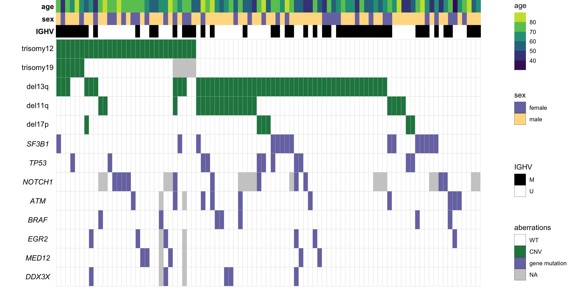
ggsave("cohortComposition.pdf", height=6, width=12)A table shown the clinical characteristics
(all cohorts combined)
patInfo <- sampleTab %>% select(encID, leukCount, cohort) %>%
  left_join(select(patMeta, Patient.ID, IGHV.status, trisomy12), by = c(encID = "Patient.ID")) %>%
  left_join(select(survT, patID, OS, died, TTT, treatedAfter, TTT, age, sex, pretreat), by = c(encID = "patID")) %>%
  select(encID, age, sex, IGHV.status, trisomy12, leukCount, OS, died, TTT, treatedAfter, pretreat, cohort)

patInfoTab <- patInfo %>% #format
  mutate(trisomy12 = ifelse(trisomy12 %in% "1", "yes", "no"),
         died = ifelse(is.na(OS),NA, ifelse(died,"yes","no")),
         treatedAfter = ifelse(is.na(TTT), NA, ifelse(treatedAfter, "yes","no")),
         pretreat = ifelse(pretreat %in% 1, "yes","no"),
         age = as.integer(age),
         OS = formatC(OS, digits=1),
         TTT = formatC(TTT, digits=1)) %>%
  mutate_all(replace_na,"NA") %>%
  arrange(cohort, encID) %>%
  dplyr::rename(ID = encID,
                IGHV = IGHV.status,
                `WBC count` = leukCount,
                `Survival time (years)` = OS,
                Died = died,
                `Time to treatment (years)` = TTT,
                `Treatment after sampling` = treatedAfter,
                `Treatment before sampling` = pretreat)
Write a csv file
write_csv2(patInfoTab, "./patInfoTab.csv")Save a latex table for supplementary table
library(xtable)
write(print(xtable(patInfoTab,
            caption = "Patient characteristics"),
      include.rownames=FALSE,
      caption.placement = "top"), file = paste0("./patInfoTab.tex"))
Summarise key statistics
Numerical variables
sumNumTab <- select(patInfo, age, leukCount, OS, TTT, cohort) %>%
  pivot_longer(-cohort) %>%
  group_by(cohort,name) %>%
  summarise(min = min(value,na.rm = TRUE), max=max(value, na.rm = TRUE), median = median(value, na.rm=TRUE))
Exploration cohort
sumNumTab %>% filter(cohort == "exploration")# A tibble: 4 x 5
# Groups: cohort [1]
cohort name min max median
<chr> <chr> <dbl> <dbl> <dbl>
1 exploration age 33.8 89.2 67.0
2 exploration leukCount 20630 413000 78710
3 exploration OS 0.0219 6.60 2.55
4 exploration TTT 0.0110 6.60 0.573Independent cohort
sumNumTab %>% filter(cohort == "independent")# A tibble: 4 x 5
# Groups: cohort [1]
cohort name min max median
<chr> <chr> <dbl> <dbl> <dbl>
1 independent age 37.3 87.5 67.8
2 independent leukCount 11500 265800 71100
3 independent OS 0.0492 10.1 3.36
4 independent TTT 0.00274 6.83 0.168Catagorical variables
sumGroupTab <- select(patInfo, sex, IGHV.status, died, treatedAfter, pretreat, cohort) %>%
  mutate_all(as.character) %>%
  pivot_longer(-cohort) %>%
  filter(!is.na(value)) %>%
  group_by(cohort,name,value) %>%
  summarise(num = length(value))
Exploration cohort
sumGroupTab %>% filter(cohort == "exploration")# A tibble: 10 x 4
# Groups: cohort, name [5]
cohort name value num
<chr> <chr> <chr> <int>
1 exploration died FALSE 80
2 exploration died TRUE 11
3 exploration IGHV.status M 47
4 exploration IGHV.status U 44
5 exploration pretreat 0 82
6 exploration pretreat 1 9
7 exploration sex f 32
8 exploration sex m 59
9 exploration treatedAfter FALSE 44
10 exploration treatedAfter TRUE 46Independent cohort
sumGroupTab %>% filter(cohort == "independent")# A tibble: 10 x 4
# Groups: cohort, name [5]
cohort name value num
<chr> <chr> <chr> <int>
1 independent died FALSE 20
2 independent died TRUE 12
3 independent IGHV.status M 1
4 independent IGHV.status U 30
5 independent pretreat 0 19
6 independent pretreat 1 13
7 independent sex f 10
8 independent sex m 22
9 independent treatedAfter FALSE 8
10 independent treatedAfter TRUE 23RNA-protein associations
Preprocess transcriptomic and proteomic data
#protCLL <- protCLL[rowData(protCLL)$uniqueMap,]

dds <- estimateSizeFactors(dds)
sampleOverlap <- intersect(colnames(protCLL), colnames(dds))
geneOverlap <- intersect(rowData(protCLL)$ensembl_gene_id, rownames(dds))
ddsSub <- dds[geneOverlap, sampleOverlap]
protSub <- protCLL[match(geneOverlap, rowData(protCLL)$ensembl_gene_id), sampleOverlap]

#how many gene don't have RNA expression at all?
noExp <- rowSums(counts(ddsSub)) == 0

#remove those genes in both datasets
ddsSub <- ddsSub[!noExp,]
protSub <- protSub[!noExp,]

#remove proteins with duplicated identifiers
protSub <- protSub[!duplicated(rowData(protSub)$name)]

geneOverlap <- intersect(rowData(protSub)$ensembl_gene_id, rownames(ddsSub))

ddsSub.vst <- varianceStabilizingTransformation(ddsSub)
Calculate correlations between protein abundance and RNA expression
rnaMat <- assay(ddsSub.vst)
proMat <- assays(protSub)[["count_combat"]]
rownames(proMat) <- rowData(protSub)$ensembl_gene_id

corTab <- lapply(geneOverlap, function(n) {
  rna <- rnaMat[n,]
  pro.raw <- proMat[n,]
  res.raw <- cor.test(rna, pro.raw, use = "pairwise.complete.obs")
  tibble(id = n,
         p = res.raw$p.value,
         coef = res.raw$estimate)
}) %>% bind_rows() %>%
  arrange(desc(coef)) %>% mutate(p.adj = p.adjust(p, method = "BH"),
                                 symbol = rowData(dds[id,])$symbol,
                                 chr = rowData(dds[id,])$chromosome)
Plot the distribution
corHistPlot <- ggplot(corTab, aes(x=coef)) + geom_histogram(position = "identity", col = colList[2], alpha =0.3, bins =50) +
  geom_vline(xintercept = 0, col = colList[1], linetype = "dashed") + xlim(-0.7,1) +
      xlab("Pearson's correlation coefficient") + theme_half +
  ggtitle("Correlation between mRNA and protein expression")
corHistPlot
Median Pearson’s correlation coefficient
median(corTab$coef)[1] 0.1836462Influence of overall protein/RNA abundance on correlation
medProt <- rowMedians(proMat,na.rm = T)
names(medProt) <- rownames(proMat)
medRNA <- rowMedians(rnaMat, na.rm = T)
names(medRNA) <- rownames(rnaMat)

plotTab <- corTab %>% mutate(rnaAbundance = medRNA[id], protAbundance = medProt[id])
plotList <- list()

plotList[["rna"]] <- plotCorScatter(plotTab,"coef","rnaAbundance",
                                    showR2 = FALSE, annoPos = "left",
                                    x_lab ="Correlation coefficient",
                                    y_lab = "Median RNA expression",
                                    title = "", dotCol = colList[5], textCol = colList[1])

plotList[["protein"]] <- plotCorScatter(plotTab,"coef","protAbundance",
                                    showR2 = FALSE, annoPos = "left",
                                    x_lab ="Correlation coefficient",
                                    y_lab = "Median protein expression",
                                    title = "", dotCol = colList[6], textCol = colList[1])

cowplot::plot_grid(plotlist = plotList, ncol =2)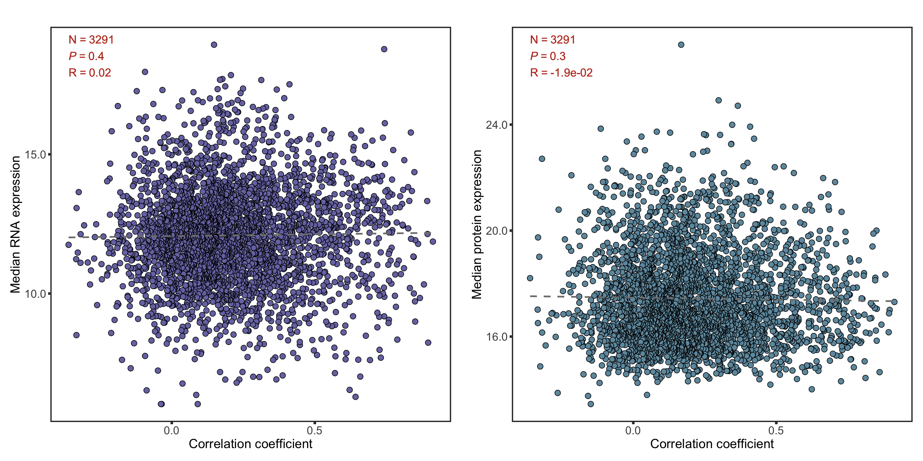
Plot protein RNA correlation for selected genes
Good correlations
geneList <- c("ZAP70","CD22","CD79A")
plotList <- lapply(geneList, function(n) {
  print(n)
  geneId <- rownames(dds)[match(n, rowData(dds)$symbol)]
  stopifnot(length(geneId) ==1)
  plotTab <- tibble(x=rnaMat[geneId,],y=proMat[geneId,], IGHV=protSub$IGHV.status)
  coef <- cor(plotTab$x, plotTab$y, use="pairwise.complete")
  annoPos <- ifelse (coef > 0, "left","right")
  plotCorScatter(plotTab, "x","y", showR2 = FALSE, annoPos = annoPos, x_lab = "RNA expression", shape = "IGHV",
                 y_lab ="Protein expression", title = n,dotCol = colList[4], textCol = colList[1], legendPos="none")
})
[1] "ZAP70"
[1] "CD22"
[1] "CD79A"goodCorPlot <- cowplot::plot_grid(plotlist = plotList, ncol =2)
goodCorPlot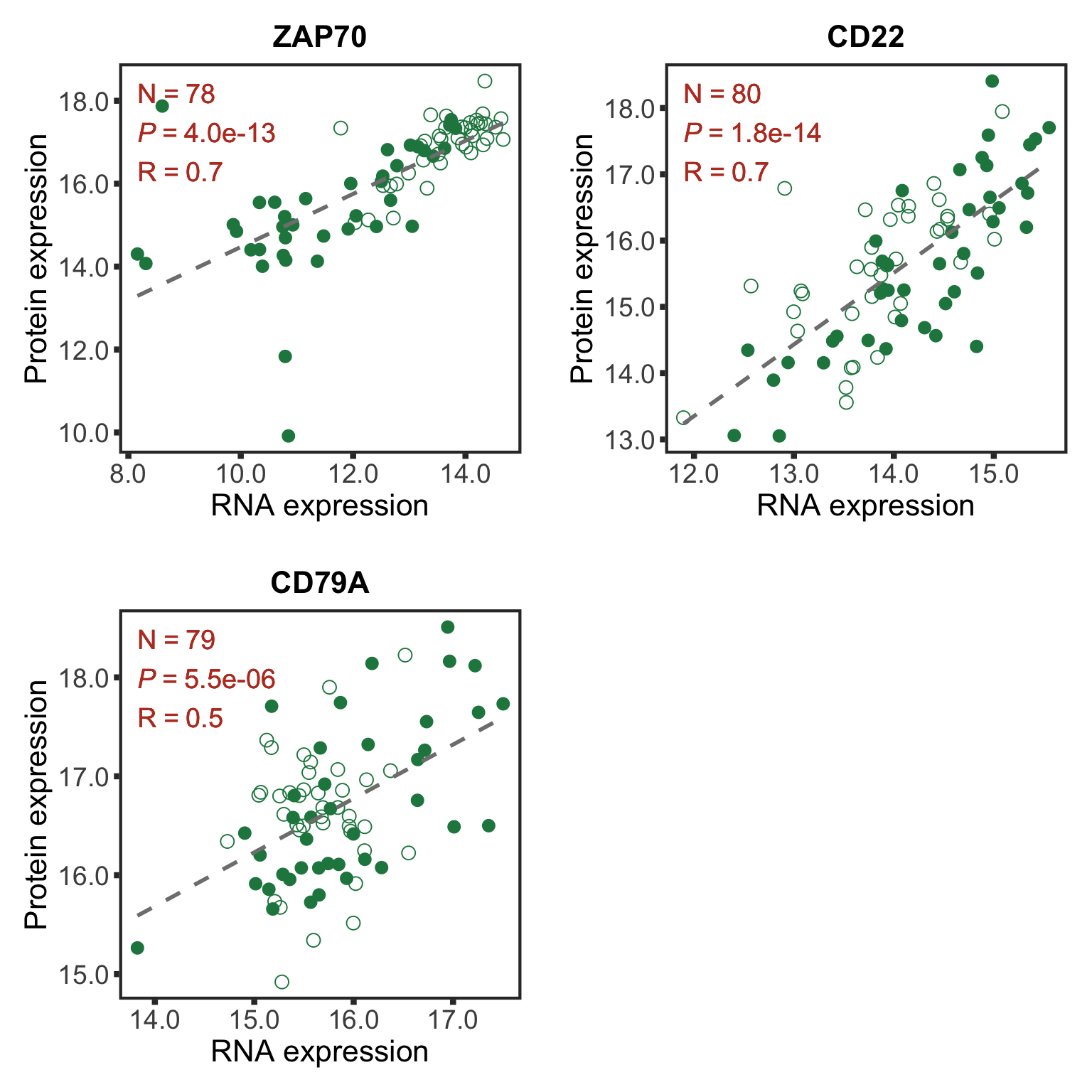 CD38 was not detected any more
Bad correlations
geneList <- c("DTNBP1","PRPF19")
plotList <- lapply(geneList, function(n) {
  geneId <- rownames(dds)[match(n, rowData(dds)$symbol)]
  stopifnot(length(geneId) ==1)
  plotTab <- tibble(x=rnaMat[geneId,],y=proMat[geneId,], IGHV=protSub$IGHV.status)
  coef <- cor(plotTab$x, plotTab$y, use="pairwise.complete")
  annoPos <- ifelse (coef > 0, "left","right")
  plotCorScatter(plotTab, "x","y", showR2 = FALSE, annoPos = annoPos, x_lab = "RNA expression",
                 y_lab ="Protein expression", title = n,dotCol = colList[4], textCol = colList[1],
                 shape = "IGHV", legendPos = "none")
})
badCorPlot <- cowplot::plot_grid(plotlist = plotList, ncol =2)
badCorPlot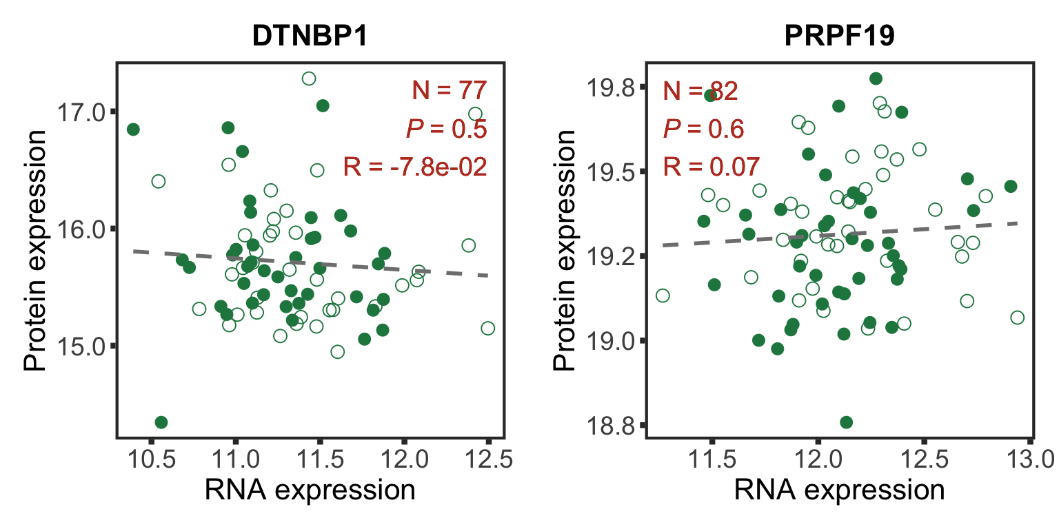
Principal component analysis
Calculate PCA
#remove genes on sex chromosomes
protCLL.sub <- protCLL[!rowData(protCLL)$chromosome_name %in% c("X","Y"),]
plotMat <- assays(protCLL.sub)[["QRILC_combat"]]
sds <- genefilter::rowSds(plotMat)
plotMat <- as.matrix(plotMat[order(sds,decreasing = TRUE),])
colAnno <- colData(protCLL)[,c("gender","IGHV.status","trisomy12")] %>%
  data.frame()
colAnno$trisomy12 <- ifelse(colAnno$trisomy12 %in% 1, "yes","no")

pcOut <- prcomp(t(plotMat), center =TRUE, scale. = TRUE)
pcRes <- pcOut$x
eigs <- pcOut$sdev^2
varExp <- structure(eigs/sum(eigs),names = colnames(pcRes))
All proteins are included for PCA analysis
Plot PC1 and PC2
plotTab <- pcRes %>% data.frame() %>% cbind(colAnno[rownames(.),]) %>%
  rownames_to_column("patID") %>% as_tibble()

plotPCA12 <- ggplot(plotTab, aes(x=PC1, y=PC2, col = trisomy12, shape = IGHV.status)) + geom_point(size=4) +
  xlab(sprintf("PC1 (%1.2f%%)",varExp[["PC1"]]*100)) +
  ylab(sprintf("PC2 (%1.2f%%)",varExp[["PC2"]]*100)) +
  scale_color_manual(values = colList) +
  scale_shape_manual(values = c(M = 16, U =1)) +
  xlim(-60,60) + ylim(-60,60) +
  theme_full + theme(legend.position = "right")

plotPCA12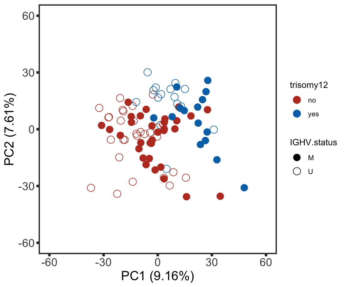
Plot PC3 and PC4
plotPCA34 <- ggplot(plotTab, aes(x=PC3, y=PC4, col = trisomy12, shape = IGHV.status)) + geom_point(size=4) +
  xlab(sprintf("PC3 (%1.2f%%)",varExp[["PC3"]]*100)) +
  ylab(sprintf("PC4 (%1.2f%%)",varExp[["PC4"]]*100)) +
  scale_color_manual(values = colList) +
  scale_shape_manual(values = c(M = 16, U =1)) +
  xlim(-60,60) + ylim(-60,60) +
  theme_full
plotPCA34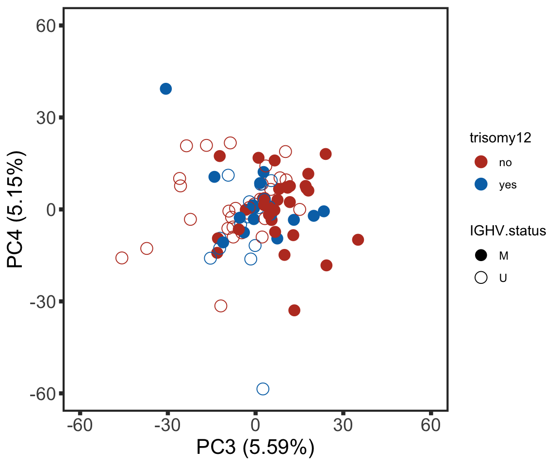
Correlation test between PCs and IGHV.status
corTab <- lapply(colnames(pcRes),  function(pc) {
  ighvCor <- t.test(pcRes[,pc] ~ colAnno$IGHV.status, var.equal=TRUE)
  tri12Cor <- t.test(pcRes[,pc] ~ colAnno$trisomy12, var.equal=TRUE)
  tibble(PC = pc,
         feature=c("IGHV", "trisomy12"),
         p = c(ighvCor$p.value, tri12Cor$p.value))
}) %>% bind_rows() %>% mutate(p.adj = p.adjust(p)) %>%
  filter(p <= 0.05) %>% arrange(p)
corTab
# A tibble: 9 x 4
PC feature p p.adj
<chr> <chr> <dbl> <dbl>
1 PC1 trisomy12 0.00000000740 0.00000135
2 PC6 trisomy12 0.0000000919 0.0000166
3 PC3 IGHV 0.0000253 0.00455
4 PC2 trisomy12 0.0000263 0.00470
5 PC5 IGHV 0.000308 0.0549
6 PC1 IGHV 0.000459 0.0813
7 PC90 trisomy12 0.0109 1
8 PC11 IGHV 0.0186 1
9 PC6 IGHV 0.0302 1 Plot PC1 and PC3
plotTab <- pcRes %>% data.frame() %>% cbind(colAnno[rownames(.),]) %>%
  rownames_to_column("patID") %>% as_tibble()

plotPCA13 <- ggplot(plotTab, aes(x=PC1, y=PC3, col = trisomy12, shape = IGHV.status)) + geom_point(size=4) +
  xlab(sprintf("PC1 (%1.2f%%)",varExp[["PC1"]]*100)) +
  ylab(sprintf("PC3 (%1.2f%%)",varExp[["PC3"]]*100)) +
  scale_color_manual(values = colList) +
  scale_shape_manual(values = c(M = 16, U =1)) +
  xlim(-60,60) + ylim(-60,60) +
  theme_full
plotPCA13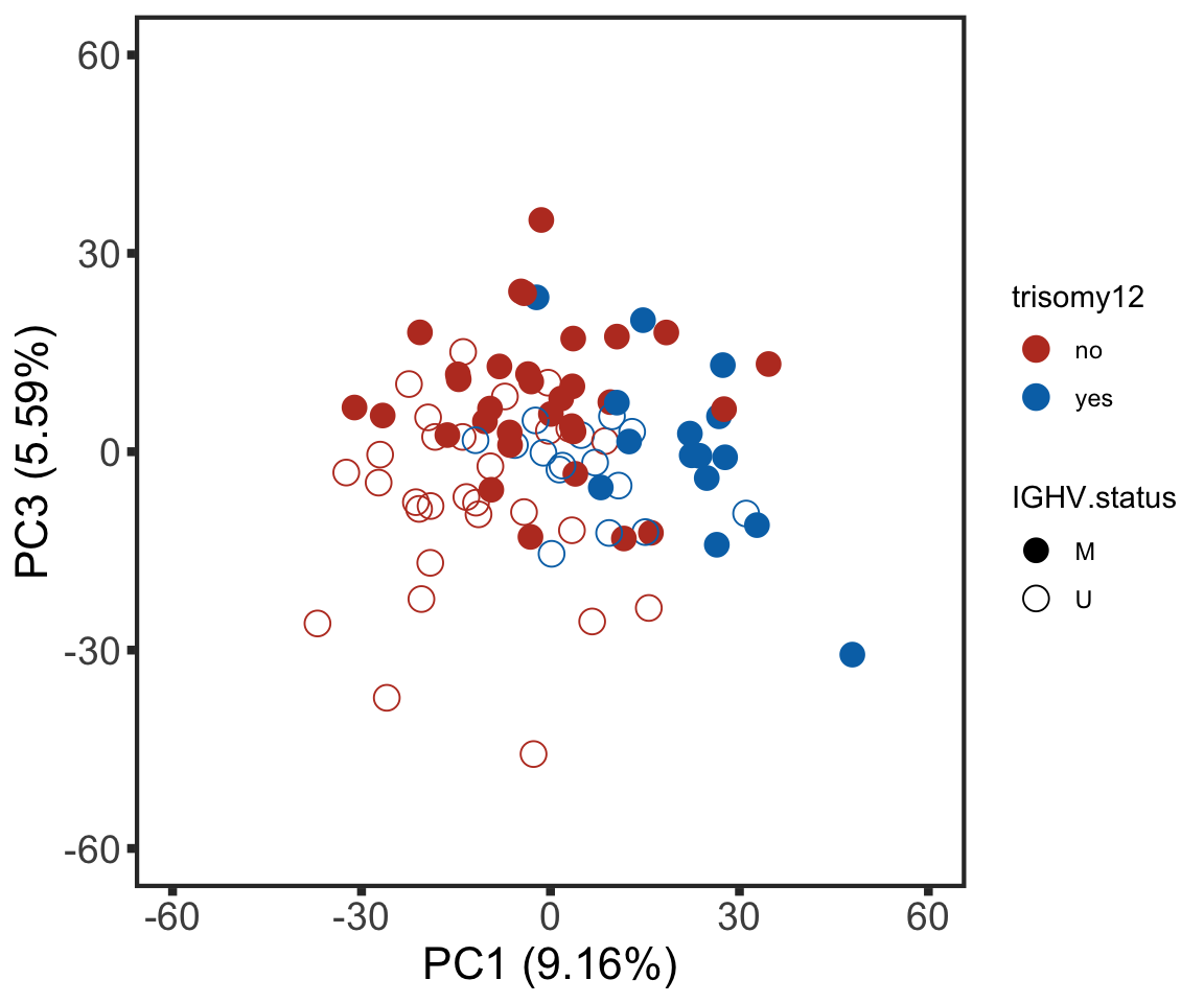
Pathway enrichment on PC1 and PC2
PC1
enRes <- list()
gmts = list(H= "../data/gmts/h.all.v6.2.symbols.gmt",
            KEGG = "../data/gmts/c2.cp.kegg.v6.2.symbols.gmt",
            C6 = "../data/gmts/c6.all.v6.2.symbols.gmt")

proMat <- assays(protCLL.sub)[["QRILC_combat"]]
iPC <- "PC1"
pc <- pcRes[,iPC][colnames(proMat)]
designMat <- model.matrix(~1+pc)
fit <- limma::lmFit(proMat, designMat)
fit2 <- eBayes(fit)
corRes <- topTable(fit2, "pc", number = Inf) %>%
  data.frame() %>% rownames_to_column("id")

inputTab <- corRes %>% filter(adj.P.Val < 0.05) %>%
  mutate(name = rowData(protCLL[id,])$hgnc_symbol) %>% filter(!is.na(name)) %>%
  distinct(name, .keep_all = TRUE) %>%
  select(name, t) %>% data.frame() %>% column_to_rownames("name")

enRes[["Proteins associated with PC1"]] <- runGSEA(inputTab, gmts$H, "page")
PC2
proMat <- assays(protCLL.sub)[["QRILC_combat"]]
iPC <- "PC2"
pc <- pcRes[,iPC][colnames(proMat)]
designMat <- model.matrix(~1+pc)
fit <- limma::lmFit(proMat, designMat)
fit2 <- eBayes(fit)
corRes <- topTable(fit2, "pc", number = Inf) %>%
  data.frame() %>% rownames_to_column("id")

inputTab <- corRes %>% filter(adj.P.Val < 0.05) %>%
  mutate(name = rowData(protCLL[id,])$hgnc_symbol) %>% filter(!is.na(name)) %>%
  distinct(name, .keep_all = TRUE) %>%
  select(name, t) %>% data.frame() %>% column_to_rownames("name")

enRes[["Proteins associated with PC2"]] <- runGSEA(inputTab, gmts$H, "page")
PC3
proMat <- assays(protCLL.sub)[["QRILC_combat"]]
iPC <- "PC3"
pc <- pcRes[,iPC][colnames(proMat)]
designMat <- model.matrix(~1+pc)
fit <- limma::lmFit(proMat, designMat)
fit2 <- eBayes(fit)
corRes <- topTable(fit2, "pc", number = Inf) %>%
  data.frame() %>% rownames_to_column("id")

inputTab <- corRes %>% filter(adj.P.Val < 0.05) %>%
  mutate(name = rowData(protCLL[id,])$hgnc_symbol) %>% filter(!is.na(name)) %>%
  distinct(name, .keep_all = TRUE) %>%
  select(name, t) %>% data.frame() %>% column_to_rownames("name")

enRes[["Proteins associated with PC3"]] <- runGSEA(inputTab, gmts$H, "page")
cowplot::plot_grid(plotEnrichmentBar(enRes[[1]], ifFDR = TRUE, pCut = 0.05, setName = "",title = "Proteins associated with PC1", removePrefix = "HALLMARK_"),
plotEnrichmentBar(enRes[[2]], ifFDR = TRUE, pCut = 0.05, setName = "", title = "Proteins associated with PC2", removePrefix = "HALLMARK_"),
plotEnrichmentBar(enRes[[3]], ifFDR = TRUE, pCut = 0.05, setName = "", title = "Proteins associated with PC3", removePrefix = "HALLMARK_"),
ncol=1,
align = "hv",
rel_heights = c(9,3,6))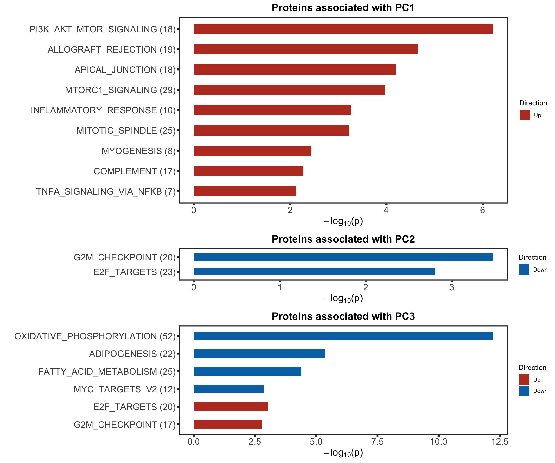
PCA analysis for batch 1 only
#remove genes on sex chromosomes
protCLL.b1 <- protCLL[!rowData(protCLL)$chromosome_name %in% c("X","Y"), filter(sampleTab, batch == "batch1")$encID]
plotMat <- assays(protCLL.b1)[["QRILC"]]
sds <- genefilter::rowSds(plotMat)
plotMat <- as.matrix(plotMat[order(sds,decreasing = TRUE),])
colAnno <- colData(protCLL)[,c("gender","IGHV.status","trisomy12")] %>%
  data.frame()
colAnno$trisomy12 <- ifelse(colAnno$trisomy12 %in% 1, "yes","no")

pcOut <- prcomp(t(plotMat), center =TRUE, scale. = TRUE)
pcRes <- pcOut$x
eigs <- pcOut$sdev^2
varExp <- structure(eigs/sum(eigs),names = colnames(pcRes))
Pathway enrichment on PC3 and PC4
PC3
enRes <- list()
proMat <- plotMat
iPC <- "PC3"
pc <- pcRes[,iPC][colnames(proMat)]
designMat <- model.matrix(~1+pc)
fit <- limma::lmFit(proMat, designMat)
fit2 <- eBayes(fit)
corRes <- topTable(fit2, "pc", number = Inf) %>%
  data.frame() %>% rownames_to_column("id")

inputTab <- corRes %>% filter(adj.P.Val < 0.05) %>%
  mutate(name = rowData(protCLL[id,])$hgnc_symbol) %>% filter(!is.na(name)) %>%
  distinct(name, .keep_all = TRUE) %>%
  select(name, t) %>% data.frame() %>% column_to_rownames("name")

enRes[["Proteins associated with PC3"]] <- runGSEA(inputTab, gmts$H, "page")
PC4
iPC <- "PC4"
pc <- pcRes[,iPC][colnames(proMat)]
designMat <- model.matrix(~1+pc)
fit <- limma::lmFit(proMat, designMat)
fit2 <- eBayes(fit)
corRes <- topTable(fit2, "pc", number = Inf) %>%
  data.frame() %>% rownames_to_column("id")

inputTab <- corRes %>% filter(adj.P.Val < 0.05) %>%
  mutate(name = rowData(protCLL[id,])$hgnc_symbol) %>% filter(!is.na(name)) %>%
  distinct(name, .keep_all = TRUE) %>%
  select(name, t) %>% data.frame() %>% column_to_rownames("name")

enRes[["Proteins associated with PC4"]] <- runGSEA(inputTab, gmts$H, "page")
cowplot::plot_grid(plotEnrichmentBar(enRes[[1]], ifFDR = TRUE, pCut = 0.05, setName = "",title = "Proteins associated with PC3", removePrefix = "HALLMARK_"),
plotEnrichmentBar(enRes[[2]], ifFDR = TRUE, pCut = 0.05, setName = "", title = "Proteins associated with PC4", removePrefix = "HALLMARK_"),
ncol=1,
align = "hv",
rel_heights = c(10,4))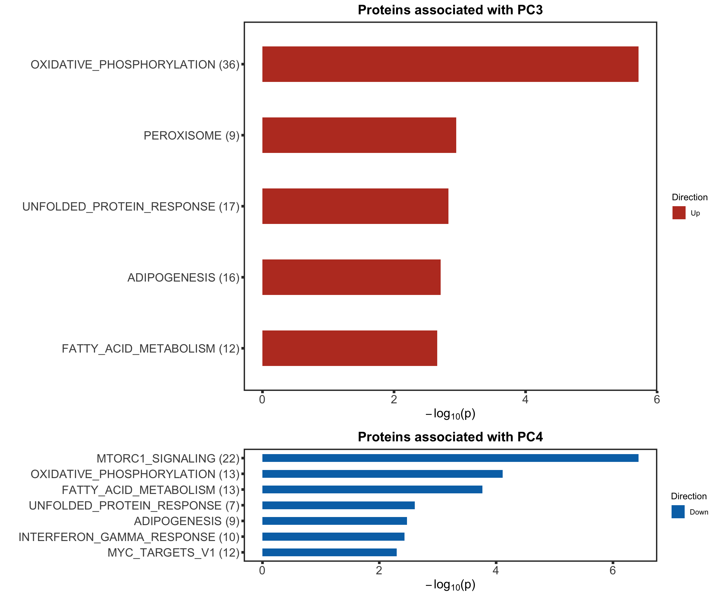
corPureTab <- lapply(colnames(pcRes)[1:20],  function(pc) {
  testTab <- pcRes[,pc, drop=FALSE] %>% as_tibble(rownames = "patID") %>%
    mutate(purity = sampleTab[match(patID, sampleTab$encID),]$purity) %>%
    filter(!is.na(purity))
  res <- cor.test(testTab[[2]], testTab[[3]])
  tibble(PC = pc,
         p= res$p.value,
         coef = res$estimate)
}) %>% bind_rows() %>% mutate(p.adj = p.adjust(p)) %>%
  filter(p <= 0.05) %>% arrange(p)
corPureTab
# A tibble: 2 x 4
PC p coef p.adj
<chr> <dbl> <dbl> <dbl>
1 PC9 0.0298 0.682 0.596
2 PC1 0.0300 -0.682 0.596usePC <- "PC1"
plotTab <- pcRes[,usePC, drop=FALSE] %>% as_tibble(rownames = "patID") %>%
mutate(purity = sampleTab[match(patID, sampleTab$encID),]$purity) %>%
filter(!is.na(purity))
ggplot(plotTab, aes_string(x=usePC,y="purity")) + geom_point() +
xlab(sprintf("%s (%1.2f%%)",usePC, varExp[[usePC]]*100)) +
geom_smooth(method ="lm") +
geom_text(x= 10,y=98, label = sprintf("P = %1.2f, Pearson's r = %1.2f", corPureTab[1,]$p, corPureTab[1,]$coef), col="darkred") +
theme_full +
ylab("tumor purity estimated by DNA methylation")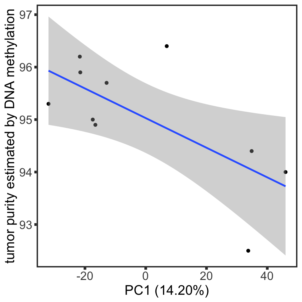
Hierarchical clustering
protCLL.sub <- protCLL[!rowData(protCLL)$chromosome_name %in% c("X","Y"),]
plotMat <- assays(protCLL.sub)[["QRILC_combat"]]
sds <- rowSds(plotMat)
plotMat <- plotMat[order(sds, decreasing = T)[1:1000],]
colAnno <- colData(protCLL)[,c("IGHV.status","trisomy12")] %>%
  data.frame()
colAnno$trisomy12 <- ifelse(colAnno$trisomy12 %in% 1, "yes","no")

plotMat <- mscale(plotMat, center = 6)

annoCol <- list(trisomy12 = c(yes = "black",no = "grey80"),
                IGHV.status = c(M = colList[3], U = colList[4]))
pheatmap::pheatmap(plotMat, annotation_col = colAnno, scale = "none",
                   clustering_method = "average", clustering_distance_cols = "correlation",
                   color = colorRampPalette(c(colList[2],"white",colList[1]))(100),
                   breaks = seq(-5,5, length.out = 101), annotation_colors = annoCol,
                   show_rownames = FALSE, show_colnames = FALSE,
                   treeheight_row = 0)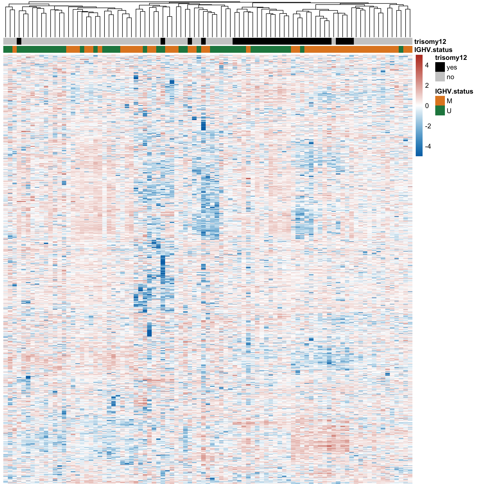
Correlation matrix
pheatmap(cor(plotMat), annotation_col = colAnno, clustering_method = "ward.D2", annotation_colors = annoCol,
         color = colorRampPalette(c(colList[2],"white",colList[1]))(100),border_color = NA,
                   breaks = seq(-1,1, length.out = 101),show_rownames = FALSE, show_colnames = FALSE)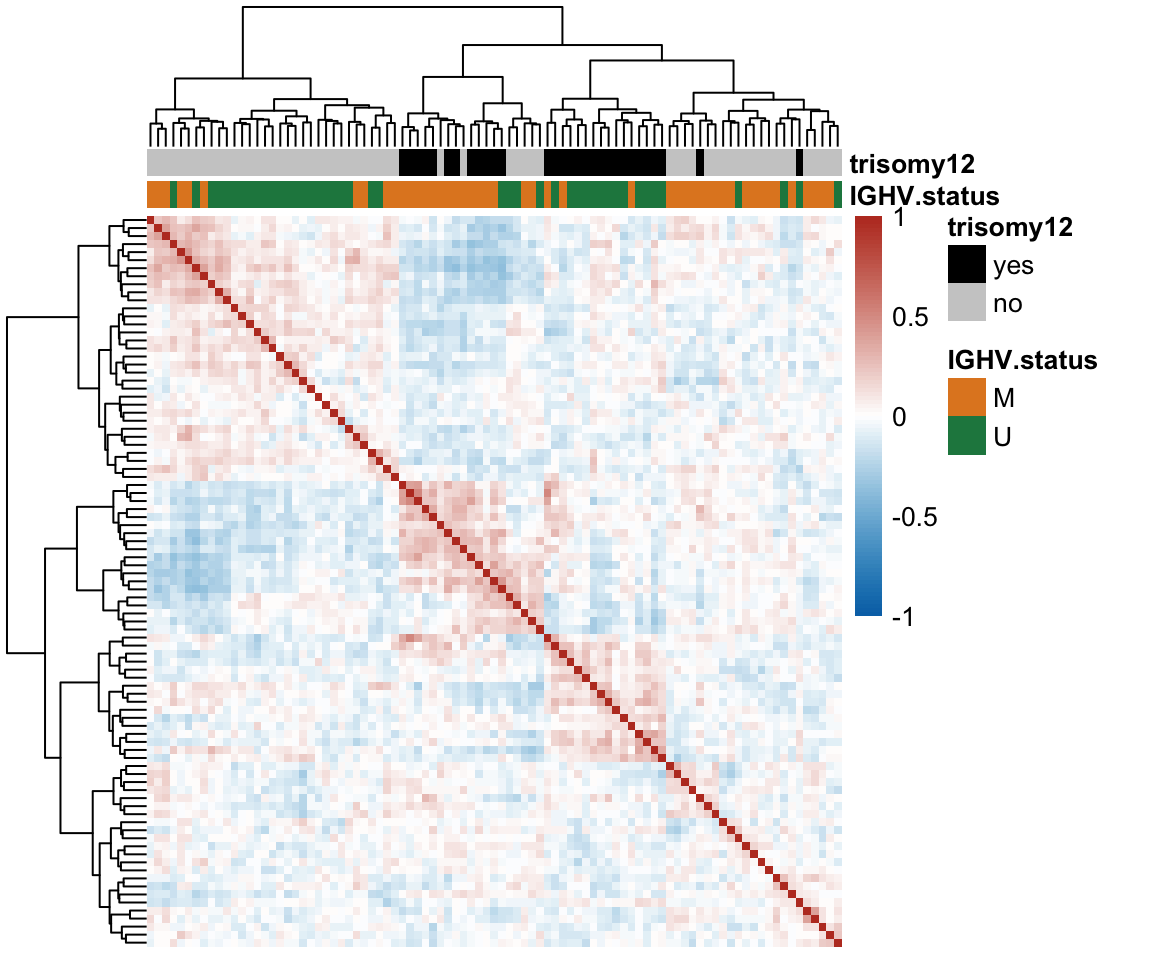
Summarise significant associations
Bar plot of number of significant associations with proteins (5% FDR)
Load the list of differentially expression proteins generated by Section 2
load("../output/deResList.RData")plotTab <- resList %>% group_by(Gene) %>%
summarise(nFDR.local = sum(adj.P.Val <= 0.05))Individual gene adjusted
plotTab <- arrange(plotTab, desc(nFDR.local)) %>% mutate(Gene = factor(Gene, levels = Gene))
numCorBar <- ggplot(plotTab, aes(x=Gene, y = nFDR.local)) + geom_bar(stat="identity",fill=colList[2]) +
  geom_text(aes(label = paste0("n=", nFDR.local)),vjust=-1,col=colList[1]) + ylim(0,1200) +
  theme_half + theme(axis.text.x = element_text(angle = 90, hjust=1, vjust=0.5)) +
  ylab("Number of associations\n(5% FDR)") + xlab("")

numCorBar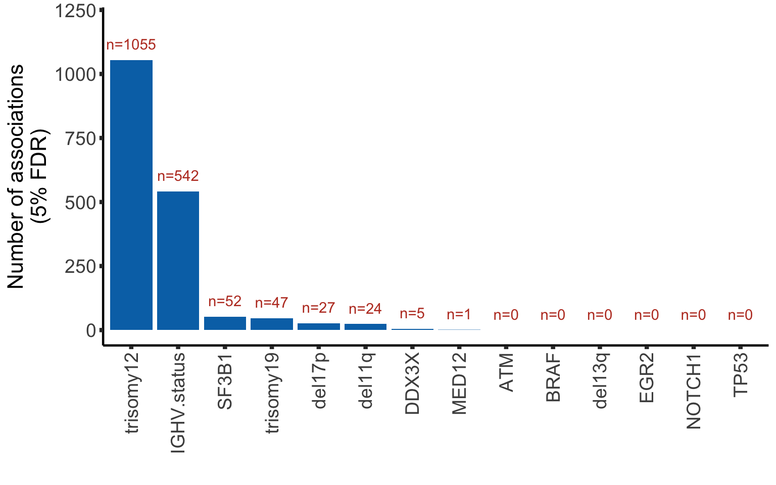
Bar plot of number of significant associations with RNAs (5% FDR)
Load the list of differentially expression proteins generated by Section 2
load("../output/deResListRNA.RData")plotTab <- resListRNA %>% group_by(Gene) %>%
summarise(nFDR.local = sum(adj.P.Val <= 0.05, na.rm=TRUE))Individual gene adjusted
plotTab <- arrange(plotTab, desc(nFDR.local)) %>% mutate(Gene = factor(Gene, levels = Gene))
numCorBarRNA <- ggplot(plotTab, aes(x=Gene, y = nFDR.local)) + geom_bar(stat="identity",fill=colList[2]) +
  geom_text(aes(label = paste0("n=", nFDR.local)),vjust=-1,col=colList[1]) + ylim(0,1500) +
  theme_half + theme(axis.text.x = element_text(angle = 90, hjust=1, vjust=0.5)) +
  ylab("Number of associations\n(5% FDR)") + xlab("")

numCorBarRNA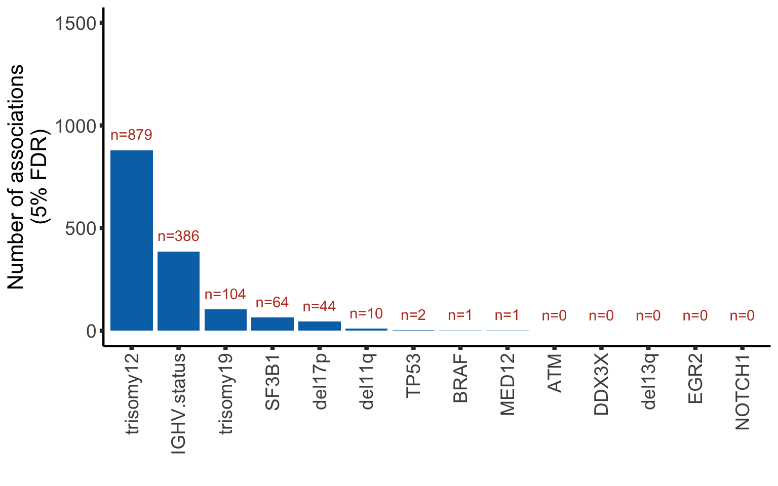
Compare differentially expressed proteins and RNAs
resList <- resList %>%
  mutate(ensembl_id = rowData(protCLL[id,])$ensembl_gene_id)
geneOverlap <- intersect(resListRNA$id, resList$ensembl_id)
rnaResList <- resListRNA %>% filter(id %in% geneOverlap) %>%
  select(id, log2FC, adj.P.Val, Gene) %>%
  dplyr::rename(rnaFC = log2FC, rnaPadj = adj.P.Val)
protResList <- resList %>% filter(ensembl_id %in% geneOverlap) %>%
  mutate(id = ensembl_id) %>%
  select(id, log2FC, adj.P.Val, Gene) %>%
  dplyr::rename(protFC = log2FC, protPadj = adj.P.Val)
comTab <- left_join(rnaResList, protResList, by =c("id","Gene"))
fdrCut <- 0.05
comTab <- comTab %>%
mutate(group = case_when(
rnaPadj < fdrCut & protPadj > fdrCut ~ "rnaOnly",
rnaPadj > fdrCut & protPadj < fdrCut ~ "proteinOnly",
rnaPadj < fdrCut & protPadj < fdrCut & rnaFC*protFC >0 ~ "both",
TRUE ~ "none"
))
plotTab <- group_by(comTab, Gene, group) %>%
summarise(n=length(id)) %>% filter(group != "none") %>%
ungroup() %>%
arrange(desc(n)) %>%
mutate(Gene = factor(Gene, levels= unique(Gene)),
group = factor(group, levels = c("rnaOnly","both","proteinOnly")))
ggplot(plotTab, aes(x=Gene, y=n, fill=group)) +
geom_bar(stat = "identity") +
theme(axis.text.x = element_text(angle = 90, hjust=1, vjust=0.5))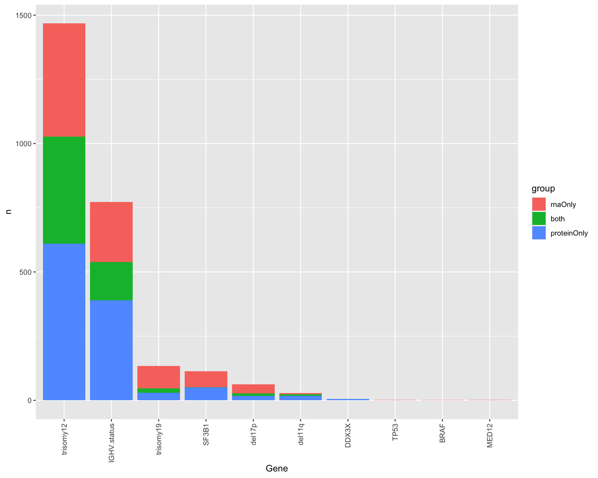
Compare timsTOF and LUMOS platforms
Load both datasets
load("../data/proteomic_explore_enc.RData")
protCLL.lumos <- protCLL[,protCLL$batch %in% "batch1"]

load("../data/proteomic_timsTOF_enc.RData")
protCLL.tims <- protCLL
How many overlapped samples?
length(intersect(colnames(protCLL.lumos), colnames(protCLL.tims)))[1] 49Number of detected proteins
Overlap of all detected proteins (< 50% missing values)
library(Vennerable)
symbolList.all <- list(LUMOS = unique(rowData(protCLL.lumos)$hgnc_symbol),
                   timsTOF = unique(rowData(protCLL.tims)$hgnc_symbol))
Vpro <- Venn(symbolList.all)
plot(Vpro, doWeights = FALSE)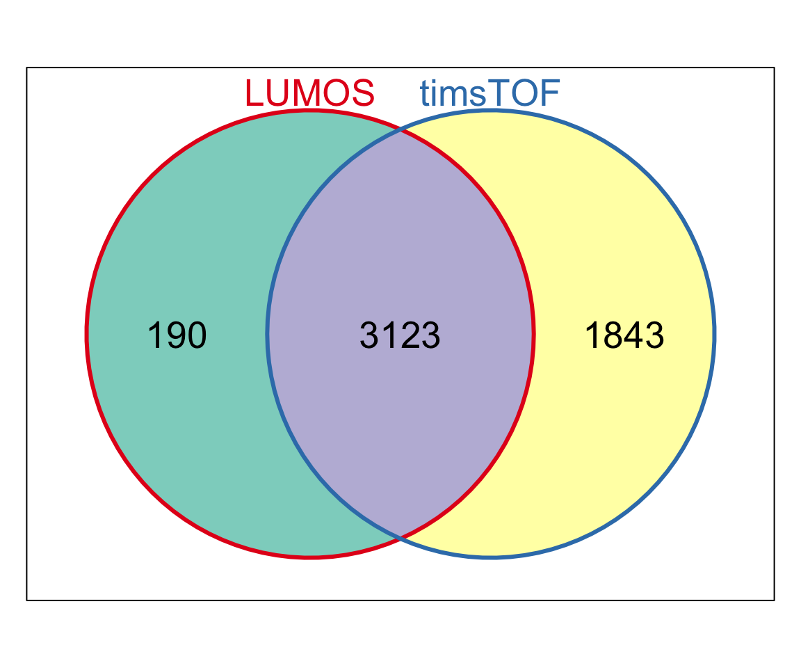
Expression distribution of common and uniquely detected proteins
commonProtein <- intersect(symbolList.all$LUMOS, symbolList.all$timsTOF)
proteinGroup <- tibble(name = commonProtein, group = "both") %>%
  bind_rows(tibble(name = setdiff(symbolList.all$LUMOS, commonProtein), group = "only in LUMOS")) %>%
  bind_rows(tibble(name = setdiff(symbolList.all$timsTOF, commonProtein), group = "only in timsTOF"))

exprTab.lumos <- assays(protCLL.lumos)[["log2Norm"]] %>% data.frame() %>%
  rownames_to_column("id") %>% mutate(name = rowData(protCLL.lumos[id,])$hgnc_symbol) %>%
  gather(key = "patID", value = "expr", -id, -name) %>%
  mutate(group = proteinGroup[match(name, proteinGroup$name),]$group,
         dataset = "LUMOS")

exprTab.tof<- assays(protCLL.tims)[["log2Norm"]] %>% data.frame() %>%
  rownames_to_column("id") %>% mutate(name = rowData(protCLL.tims[id,])$hgnc_symbol) %>%
  gather(key = "patID", value = "expr", -id, -name) %>%
  mutate(group = proteinGroup[match(name, proteinGroup$name),]$group,
         dataset = "timsTOF")

exprTab <- bind_rows(exprTab.lumos, exprTab.tof)
ggplot(exprTab, aes(x = expr, fill = group)) +
  geom_histogram(position = "identity", alpha = 0.5, bins=100, col = "grey50") +
  facet_wrap(~dataset) +
  xlab("log2(protein counts)") +
  theme_full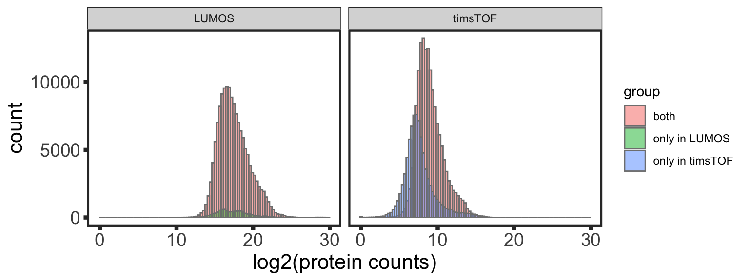
Correlations of commonly detected proteins
Pearson correlation coefficient
sumProtein <- filter(exprTab, group == "both") %>%
  filter(!is.na(expr)) %>% group_by(id) %>%
  summarise(nLUMOS = sum(dataset == "LUMOS"),nTOF = sum(dataset=="timsTOF")) %>%
  filter(nLUMOS >= 10 & nTOF >=10 )

testRes <- filter(exprTab, group == "both", id %in% sumProtein$id) %>%
  mutate(expr = log(expr)) %>%
  spread(key = dataset, value = expr) %>%
  group_by(id) %>% nest() %>%
  mutate(m = map(data, ~cor.test(~LUMOS+timsTOF,.))) %>%
  mutate(res = map(m, broom::tidy)) %>%
  unnest(res)

ggplot(testRes, aes(x=estimate)) + geom_histogram(position = "identity", fill = colList[3], col = "grey50", alpha =0.3, bins =100) +
  geom_vline(xintercept = 0, col = "red", linetype = "dashed") +
  xlab("Pearson's correlation coefficient") +
  theme_full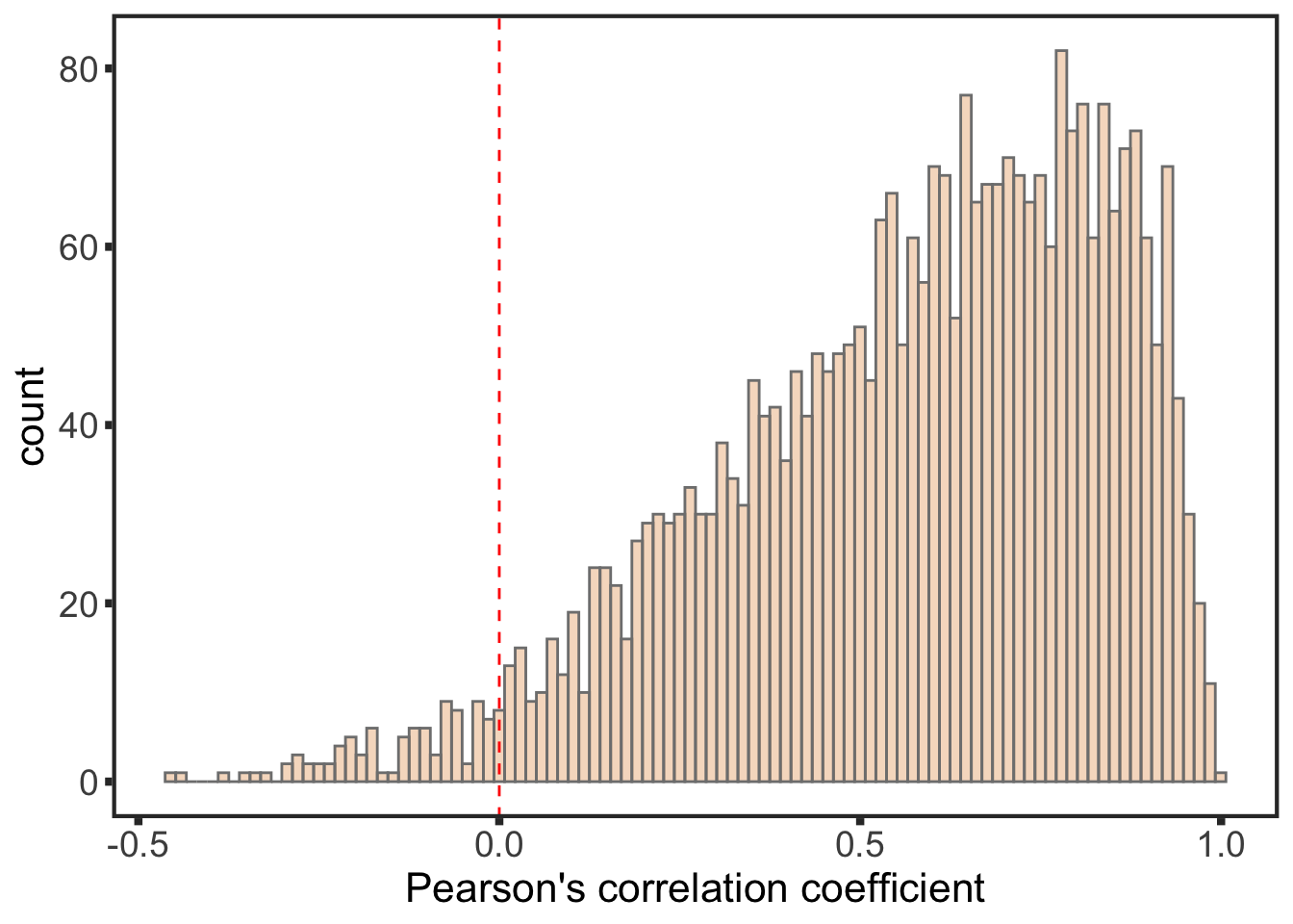
Correlation of top 10 PCs
library(corrplot)
overSample <- intersect(colnames(protCLL.lumos), colnames(protCLL.tims))
pcResLumos <- prcomp(t(assays(protCLL.lumos[,overSample])[["QRILC"]]), center = TRUE, scale. = TRUE)
pcResTims <- prcomp(t(assays(protCLL.tims[,overSample])[["QRILC"]]), center = TRUE, scale. = TRUE)
pcLumos <- pcResLumos$x[,1:10] %>% as.matrix()
pcTims <- pcResTims$x[,1:10] %>% as.matrix()
Variance explained by top10 PCs
eigsLumos <- pcResLumos$sdev^2
eigsTims <- pcResTims$sdev^2
sumVarExpr <- structure(c(sum(eigsLumos[1:10])/sum(eigsLumos), sum(eigsTims[1:10])/sum(eigsLumos)), names = c("LUMOS","timsTOF"))
sumVarExpr
LUMOS timsTOF
0.6050520 0.8697672 #function to do correlation test on matrix
cor.mtest <- function(mat1, mat2=NULL, conf.level = 0.99) {
if(is.null (mat2)) mat2 <- mat1
mat1 <- as.matrix(mat1)
mat2 <- as.matrix(mat2)
stopifnot(ncol(mat1) == ncol(mat2))
n1 <- nrow(mat1)
n2 <- nrow(mat2)
p.mat <- cor.rho <- matrix(NA, n1, n2)
for (i in 1:n1) {
for (j in 1:n2) {
tmp <- cor.test(mat1[i, ], mat2[j, ], conf.level = conf.level,
use="pairwise.complete.obs",method="pearson")
p.mat[i, j] <- tmp$p.value
cor.rho[i, j] <- abs(tmp$estimate[[1]])
}
}
colnames(cor.rho) <- colnames(p.mat) <- rownames(mat2)
rownames(cor.rho) <- rownames(p.mat) <- rownames(mat1)
return(list(cor.rho, p.mat))
}
featureCor <- cor.mtest(t(pcLumos), t(pcTims))
#correlation heatmap
corrplot(featureCor[[1]],order="original",p.mat = featureCor[[2]],sig.level = 0.01, cl.lim = c(0,1))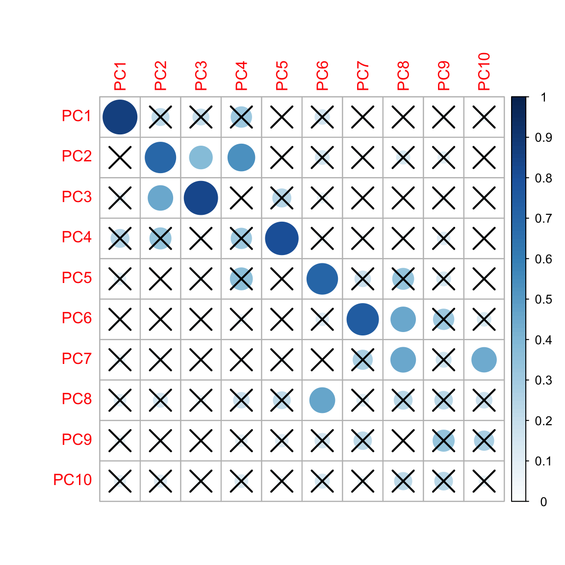
Assemble figure
designPlot <- draw_image("../data/Fig1A.png")
p <- ggdraw() + designPlot

leftCol <- plot_grid(p,
                     plot_grid(plotPCA12, plotPCA34, ncol=2, rel_widths = c(.45,0.55)),
                     plot_grid(numCorBar,NULL,rel_widths = c(0.8,0.2),ncol=2), ncol = 1,
                     labels = c("A","E","F"), label_size = 20, vjust = c(1.5, 0,-0.1),
                     rel_heights = c(1.2,1,1))


rightCol <- plot_grid(corHistPlot,
                       goodCorPlot,
                       badCorPlot, ncol=1, rel_heights = c(0.28,0.48,0.24), labels = c("B","C","D"), label_size = 20)
#pdf("test.pdf", height = 13, width = 18)
plot_grid(leftCol, rightCol, rel_widths = c(0.6, 0.4))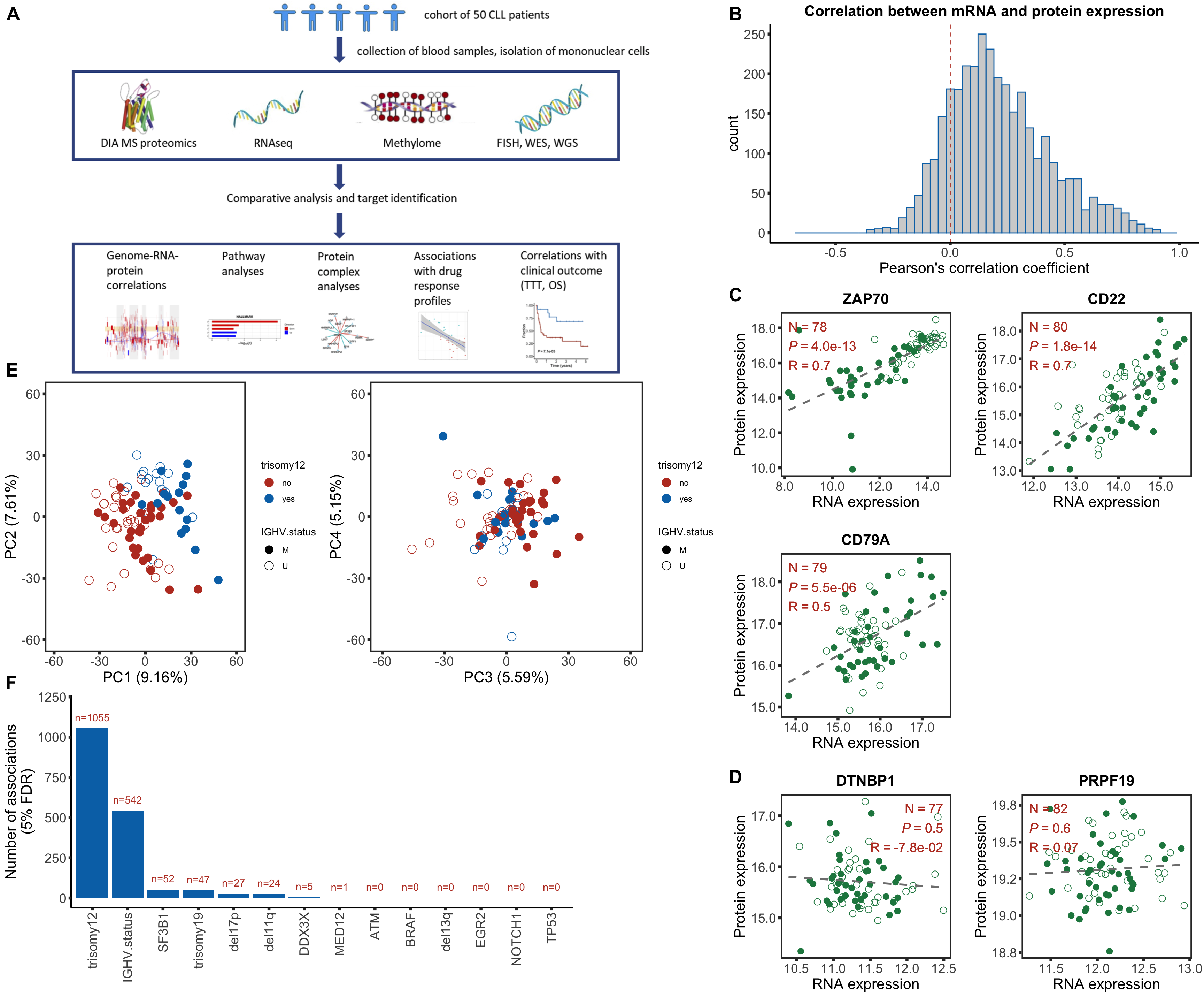
#dev.off()Supplementary, overview of the indepdent cohort composition
load("../data/proteomic_independent_enc.RData")
protCLL <- protCLL[,colnames(protCLL) %in% patMeta$Patient.ID]
Genomic matrix
Get mutations with at least 5 cases
geneMat <-  patMeta[match(colnames(protCLL), patMeta$Patient.ID),] %>%
  select(-IGHV.status, -Methylation_Cluster) %>%
  mutate_if(is.factor, as.character) %>%
  mutate_at(vars(-Patient.ID), as.numeric) %>% #assign a few unknown mutated cases to wildtype
  data.frame() %>% column_to_rownames("Patient.ID")


#geneMat <- geneMat[,apply(geneMat,2, function(x) sum(x %in% 1, na.rm = TRUE))>=5]
#dim(geneMat)
Mutations that will be tested
#Remove some dubious annotations
geneMat <- geneMat[,c(useGeneForComposition,"U1")]
colnames(geneMat)
[1] "del11q" "del13q" "del17p" "trisomy12" "trisomy19" "ATM"
[7] "BRAF" "DDX3X" "EGR2" "MED12" "NOTCH1" "SF3B1"
[13] "TP53" "U1" Dimension
dim(geneMat)[1] 26 14Plot to summarise genomic background
Separate CNV table and mutation table
cnvCol <- colnames(geneMat)[grepl("del|trisomy",colnames(geneMat))]
cnvMat <- geneMat[,cnvCol]
mutMat <- geneMat[,!colnames(geneMat) %in% cnvCol]
cnvMat <- cnvMat[,names(sort(colSums(cnvMat == 1,na.rm=TRUE)))]
#
#Manually assign CNV feature order for better visualization
#cnvMat <- cnvMat[,c("del17p","del11q","del13q","trisomy19","trisomy12")]


mutMat <- mutMat[,names(sort(colSums(mutMat == 1, na.rm=TRUE)))]
geneMat <- cbind(mutMat,cnvMat)
geneMat[is.na(geneMat)] <- -1
Sort patient based on CNVs
sortTab <- function(sumTab) {
  i <- ncol(sumTab)
  #print(i)
  if (i == 1) {
    return(rownames(sumTab)[order(sumTab[,i])])
  }
  allLevel <- sort(unique(sumTab[,i]))
  orderRow <- lapply(allLevel, function(n) {
    sortTab(sumTab[sumTab[,i] %in% n, seq(1,i-1), drop = FALSE])
  }) %>% unlist() %>% c()
  return(orderRow)
}

sortedPat <- rev(sortTab(geneMat))
Prepare table for plot
plotTab <- geneMat %>% as_tibble(rownames="patID") %>% mutate_all(as.character) %>%
  pivot_longer(-patID, names_to = "var", values_to = "value") %>%
  mutate(status = case_when(
    value == -1 ~ "NA",
    value == 0 ~ "WT",
    value == 1 & var %in% cnvCol ~ "CNV",
    value == 1 & !var %in% cnvCol ~ "gene mutation"
  )) %>%
  mutate(var = factor(var, levels = c(colnames(mutMat),colnames(cnvMat))),
         patID = factor(patID, levels = sortedPat),
         status = factor(status, levels =c("WT","CNV","gene mutation","NA")))

formatedName <- lapply(levels(plotTab$var), function(n) {
  if(n %in% cnvCol) {
    n
  } else {
    bquote(italic(.(n)))
  }
})
Plot mutation matrix
pMain <- ggplot(plotTab, aes(x=patID, y = var, fill = status)) +
  geom_tile(color = "grey80") +
  theme_void() +
  scale_fill_manual(values = c("gene mutation" = colList[5],
                               "CNV"= colList[4],
                               "WT" ="white",
                               "NA" = "grey80"),
                    name = "aberrations") +
  scale_y_discrete(labels = formatedName) +
  theme(axis.text.x =  element_blank(),
        axis.text.y = element_text(size=11, face = "bold"),
        axis.ticks.length.y = unit(0.05,"npc")) +
  ylab("") + xlab("")
#pMain
Annotation matrix
IGHV status
ighvTab <- select(patMeta, Patient.ID, IGHV.status) %>%
  mutate(patID = Patient.ID, status = IGHV.status, type = "IGHV") %>%
  filter(patID %in% sortedPat) %>%
  mutate(patID = factor(patID, levels = sortedPat)) %>%
  select(patID, type, status) %>%
  mutate(status = ifelse(is.na(status),"NA",status))

pIGHV <- ggplot(ighvTab, aes(x=patID, y = type, fill = status)) +
  geom_tile(color = NA) +
  theme_void() + xlab("") + ylab("") +
  coord_cartesian(expand = FALSE) +
  scale_fill_manual(values = c(M="black",U="white", "NA" = "grey80"), name = "IGHV") +
  theme(axis.text.y = element_text(face = "bold", size=11),
        axis.ticks.length.y = unit(0.05,"npc"))

table(ighvTab$status)
 M NA  U
1 1 24 #pIGHVSex
sexTab <- select(survT, patID, sex) %>%
  mutate(status = as.character(sex), type = "sex") %>%
  filter(patID %in% sortedPat) %>%
  mutate(patID = factor(patID, levels = sortedPat),
         status = case_when(status %in% "m" ~ "male",
                            status %in% "f" ~ "female")) %>%
  select(patID, type, status)

pSex <- ggplot(sexTab, aes(x=patID, y = type, fill = status)) +
  geom_tile(color = NA) +
  theme_void() + xlab("") +  ylab("") +
  coord_cartesian(expand = FALSE) +
  scale_fill_manual(values = c(male=colList[7],female=colList[5]), name = "sex") +
  theme(axis.text.y = element_text(face = "bold",size=11),
        axis.ticks.length.y = unit(0.05,"npc"))
#pSex
table(sexTab$status)
female   male
    10     16
Pretreatment
treatTab <- survT %>% filter(patID %in% sortedPat) %>%
  select(patID, pretreat) %>%
  mutate(treatment = case_when(pretreat %in% 1 ~ "yes",
                               pretreat %in% 0 ~ "no",
                               is.na(pretreat) ~ "NA")) %>%
  mutate(status = as.character(treatment), type = "treatment") %>%
  mutate(patID = factor(patID, levels = sortedPat)) %>%
  select(patID, type, status)


pTreat <- ggplot(treatTab, aes(x=patID, y = type, fill = status)) +
  geom_tile(color = NA) +
  theme_void() + xlab("") +  ylab("") +
  coord_cartesian(expand = FALSE) +
  scale_fill_manual(values = c(yes = "black", no = "white","NA" = "grey80"), name = "treatment") +
  theme(axis.text.y = element_text(face = "bold",size=11),
        axis.ticks.length.y = unit(0.05,"npc"))
#pTreat
Age
agePlotTab <- survT %>% filter(patID %in% sortedPat) %>%
  select(patID, age) %>%
  mutate( status = age, type = "age") %>%
  mutate(patID = factor(patID, levels = sortedPat)) %>%
  select(patID, type, status)


pAge <- ggplot(agePlotTab, aes(x=patID, y = type, fill = status)) +
  geom_tile(color = NA) +
  theme_void() + xlab("") +  ylab("") +
  coord_cartesian(expand = FALSE) +
  scale_fill_viridis_b(name = "age") +
  theme(axis.text.y = element_text(face = "bold",size=11),
        axis.ticks.length.y = unit(0.05,"npc"))
#pAge
Combine all plots
lMain <- get_legend(pMain + geom_tile(color = "black") )
lAge <- get_legend(pAge + geom_tile(color = "black") )
lSex <- get_legend(pSex+ geom_tile(color = "black") )
lIGHV <- get_legend(pIGHV+ geom_tile(color = "black") )
lTreat <- get_legend(pTreat+ geom_tile(color = "black") )

noLegend <- theme(legend.position = "none")
mainPlot <- plot_grid(pAge + noLegend, pSex + noLegend,
                              pIGHV + noLegend,
                     pMain + noLegend, ncol=1, align = "v",
                     rel_heights = c(rep(1,3),20))


legendPlot <- plot_grid(lAge, lSex, lIGHV, lMain,ncol=1, align = "hv")

plot_grid(mainPlot, NULL, plot_grid(legendPlot, ncol=1), ncol=3, rel_widths = c(1,0.05, 0.15))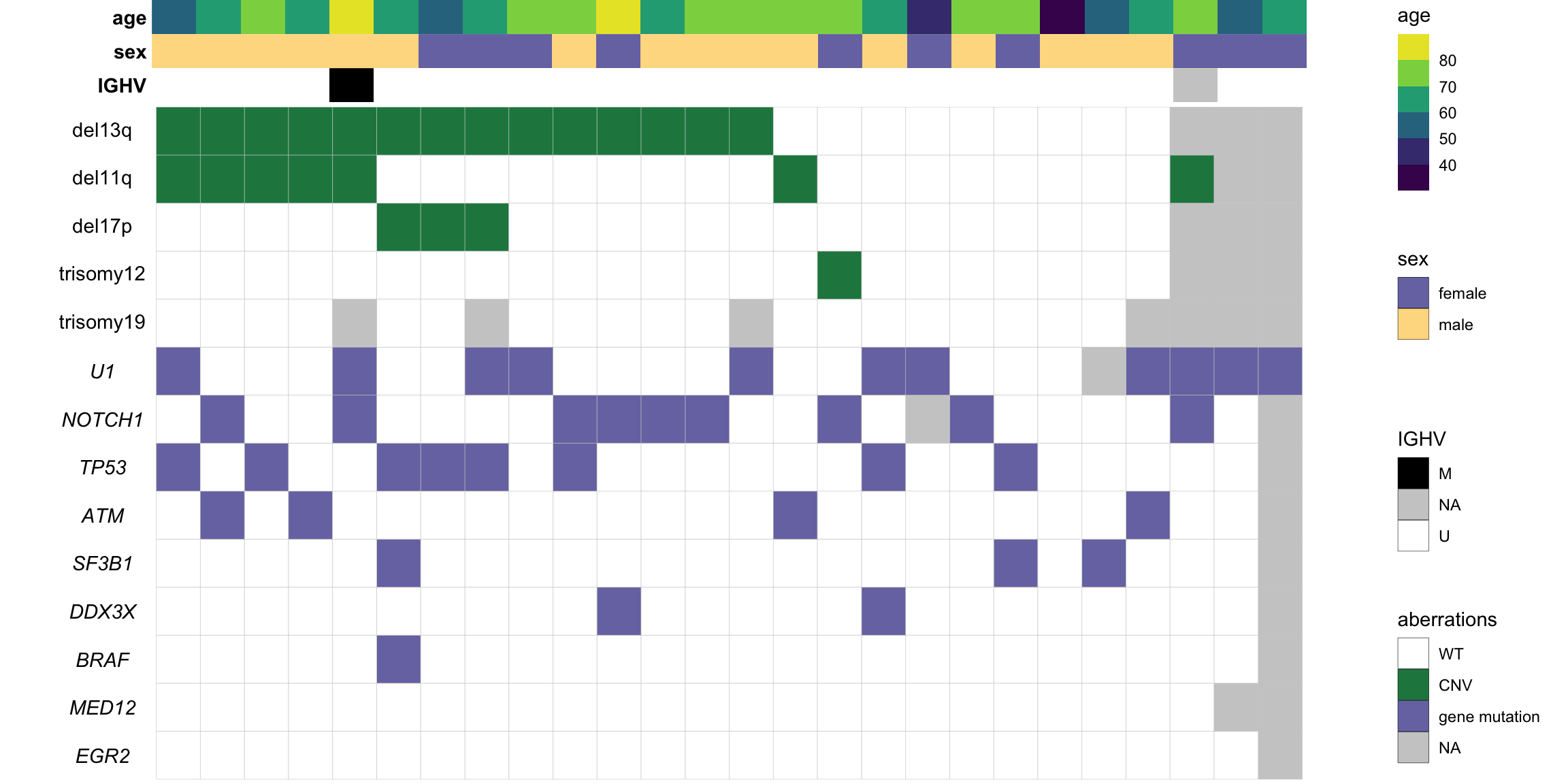
ggsave("cohortComposition_batch2.pdf", height=6, width=12)
sessionInfo()R version 4.0.2 (2020-06-22)
Platform: x86_64-apple-darwin17.0 (64-bit)
Running under: macOS 10.16
Matrix products: default
BLAS: /Library/Frameworks/R.framework/Versions/4.0/Resources/lib/libRblas.dylib
LAPACK: /Library/Frameworks/R.framework/Versions/4.0/Resources/lib/libRlapack.dylib
locale:
[1] en_US.UTF-8/en_US.UTF-8/en_US.UTF-8/C/en_US.UTF-8/en_US.UTF-8
attached base packages:
[1] parallel stats4 stats graphics grDevices utils datasets
[8] methods base
other attached packages:
[1] corrplot_0.84 Vennerable_3.1.0.9000
[3] piano_2.4.0 xtable_1.8-4
[5] latex2exp_0.4.0 forcats_0.5.1
[7] stringr_1.4.0 dplyr_1.0.5
[9] purrr_0.3.4 readr_1.4.0
[11] tidyr_1.1.3 tibble_3.1.0
[13] ggplot2_3.3.3 tidyverse_1.3.0
[15] pheatmap_1.0.12 proDA_1.2.0
[17] cowplot_1.1.1 DESeq2_1.28.1
[19] SummarizedExperiment_1.18.2 DelayedArray_0.14.1
[21] matrixStats_0.58.0 Biobase_2.48.0
[23] GenomicRanges_1.40.0 GenomeInfoDb_1.24.2
[25] IRanges_2.22.2 S4Vectors_0.26.1
[27] BiocGenerics_0.34.0 limma_3.44.3
loaded via a namespace (and not attached):
[1] readxl_1.3.1 backports_1.2.1 fastmatch_1.1-0
[4] workflowr_1.6.2 plyr_1.8.6 igraph_1.2.6
[7] shinydashboard_0.7.1 splines_4.0.2 BiocParallel_1.22.0
[10] digest_0.6.27 htmltools_0.5.1.1 magick_2.7.0
[13] fansi_0.4.2 magrittr_2.0.1 memoise_2.0.0
[16] cluster_2.1.1 annotate_1.66.0 modelr_0.1.8
[19] colorspace_2.0-0 blob_1.2.1 rvest_1.0.0
[22] haven_2.3.1 xfun_0.21 crayon_1.4.1
[25] RCurl_1.98-1.2 jsonlite_1.7.2 graph_1.66.0
[28] genefilter_1.70.0 survival_3.2-7 glue_1.4.2
[31] gtable_0.3.0 zlibbioc_1.34.0 XVector_0.28.0
[34] scales_1.1.1 DBI_1.1.1 relations_0.6-9
[37] Rcpp_1.0.6 viridisLite_0.3.0 bit_4.0.4
[40] DT_0.17 htmlwidgets_1.5.3 httr_1.4.2
[43] fgsea_1.14.0 gplots_3.1.1 RColorBrewer_1.1-2
[46] ellipsis_0.3.1 pkgconfig_2.0.3 XML_3.99-0.5
[49] farver_2.1.0 sass_0.3.1 dbplyr_2.1.0
[52] locfit_1.5-9.4 utf8_1.1.4 reshape2_1.4.4
[55] tidyselect_1.1.0 labeling_0.4.2 rlang_0.4.10
[58] later_1.1.0.1 AnnotationDbi_1.50.3 munsell_0.5.0
[61] cellranger_1.1.0 tools_4.0.2 visNetwork_2.0.9
[64] cachem_1.0.4 cli_2.3.1 generics_0.1.0
[67] RSQLite_2.2.3 broom_0.7.5 evaluate_0.14
[70] fastmap_1.1.0 yaml_2.2.1 knitr_1.31
[73] bit64_4.0.5 fs_1.5.0 caTools_1.18.1
[76] RBGL_1.64.0 nlme_3.1-152 mime_0.10
[79] slam_0.1-48 xml2_1.3.2 compiler_4.0.2
[82] rstudioapi_0.13 marray_1.66.0 reprex_1.0.0
[85] geneplotter_1.66.0 bslib_0.2.4 stringi_1.5.3
[88] highr_0.8 lattice_0.20-41 Matrix_1.3-2
[91] shinyjs_2.0.0 vctrs_0.3.6 pillar_1.5.1
[94] lifecycle_1.0.0 jquerylib_0.1.3 data.table_1.14.0
[97] bitops_1.0-6 httpuv_1.5.5 R6_2.5.0
[100] promises_1.2.0.1 KernSmooth_2.23-18 gridExtra_2.3
[103] gtools_3.8.2 assertthat_0.2.1 rprojroot_2.0.2
[106] withr_2.4.1 GenomeInfoDbData_1.2.3 mgcv_1.8-34
[109] hms_1.0.0 grid_4.0.2 rmarkdown_2.7
[112] git2r_0.28.0 sets_1.0-18 shiny_1.6.0
[115] lubridate_1.7.10