Visualizing gene dosage effect on protein and RNA level
Log2 protein counts
protExprTab <- sumToTidy(protCLL) %>%
  filter(chromosome_name == "12") %>%
  mutate(id = ensembl_gene_id, patID = colID, expr = log2Norm_combat, type = "Protein") %>%
  select(id, patID, expr, type)
Log2 RNA seq counts
rnaExprTab <- counts(dds[rownames(dds) %in% protExprTab$id,
                            colnames(dds) %in% protExprTab$patID], normalized= TRUE) %>%
  as_tibble(rownames = "id") %>%
  pivot_longer(-id, names_to = "patID", values_to = "count") %>%
  mutate(expr = log2(count)) %>%
  select(id, patID, expr) %>% mutate(type = "RNA")
comExprTab <- bind_rows(rnaExprTab, protExprTab) %>%
  mutate(trisomy12 = patMeta[match(patID, patMeta$Patient.ID),]$trisomy12) %>%
  filter(!is.na(trisomy12)) %>% mutate(cnv = ifelse(trisomy12 %in% 1, "trisomy12","WT"))
Proteins/RNAs on Chr12 have higher expressions in trisomy12 samples compared to other samples
plotTab <- comExprTab %>%
  group_by(id,type) %>% mutate(zscore = (expr-mean(expr))/sd(expr)) %>%
  group_by(id, cnv, type) %>% summarise(meanExpr = mean(zscore, na.rm=TRUE)) %>%
  ungroup()

dosagePlot <- ggplot(plotTab, aes(x=meanExpr, fill = cnv, col=cnv)) +
  geom_histogram(position = "identity", alpha=0.5, bins=30) + facet_wrap(~type, scale = "fixed") +
  scale_fill_manual(values = c(WT = "grey80", trisomy12 = colList[1]), name = "") +
  scale_color_manual(values = c(WT = "grey80", trisomy12 = colList[1]), name = "") +
  #xlim(-1,1) +
  theme_full + xlab("Mean Z-score") +
  theme(strip.text = element_text(size =20))

dosagePlot

The variation of expression is higher in RNA than protein
For proteins/RNA on chr12
plotTab <- comExprTab %>%
  group_by(id, type) %>% summarise(varExp = sd(expr, na.rm=TRUE)) %>%
  ungroup()

ggplot(plotTab, aes(x=varExp,  fill = type, col=type)) +
  geom_histogram(position = "identity", alpha=0.5) +
  scale_fill_manual(values = c(RNA = colList[4], Protein = colList[5]), name = "") +
  scale_color_manual(values = c(RNA = colList[4], Protein = colList[5]), name = "") +
  theme_full + xlab("Standard deviation of expression")

The overall scale of change is higher in RNA expression than protein expression
plotTab <- comExprTab%>%
  group_by(id, type, cnv) %>% summarise(meanExp = mean(expr, na.rm=TRUE)) %>%
  ungroup() %>% spread(key = cnv, value = meanExp) %>%
  mutate(log2FC = trisomy12-WT)

ggplot(plotTab, aes(x=log2FC, fill = type, col=type)) +
  geom_histogram(position = "identity", alpha=0.5, bins = 100) +
  scale_fill_manual(values = c(RNA = colList[3], Protein = colList[4]), name = "") +
  scale_color_manual(values = c(RNA = colList[3], Protein = colList[4]), name = "") +
  #coord_cartesian(xlim=c(-0.25,0.25))+
  geom_vline(xintercept = 0, col = colList[1], linetype = "dashed") +
  theme_full + xlab("log2 Fold Change")

Analyzing buffering effect
Detect buffered and non-buffered proteins
Preprocessing protein and RNA data
#subset samples and genes
overSampe <- intersect(colnames(ddsCLL), colnames(protCLL))
overGene <- intersect(rownames(ddsCLL), rowData(protCLL)$ensembl_gene_id)
ddsSub <- ddsCLL[overGene, overSampe]
protSub <- protCLL[match(overGene, rowData(protCLL)$ensembl_gene_id),overSampe]
rowData(ddsSub)$uniprotID <- rownames(protSub)[match(rownames(ddsSub),rowData(protSub)$ensembl_gene_id)]

#vst
ddsSub.vst <- ddsSub
assay(ddsSub.vst) <- log2(counts(ddsSub, normalized=TRUE) +1)
#ddsSub.vst <- varianceStabilizingTransformation(ddsSub)
Differential expression on RNA level
#design(ddsSub) <- ~ trisomy12 + IGHV
#deRes <- DESeq(ddsSub, betaPrior = TRUE)
rnaRes <- resListRNA %>% filter(Gene == "trisomy12") %>%
  mutate(Chr = rowData(dds[id,])$chromosome) %>%
  #filter(Chr == "12") %>%
  #mutate(adj.P.Val = p.adjust(P.Value, method = "BH")) %>%
  dplyr::rename(geneID = id, log2FC.rna = log2FC,
                pvalue.rna = P.Value, padj.rna = adj.P.Val, stat.rna= t) %>%
  select(geneID, log2FC.rna, pvalue.rna, padj.rna, stat.rna)
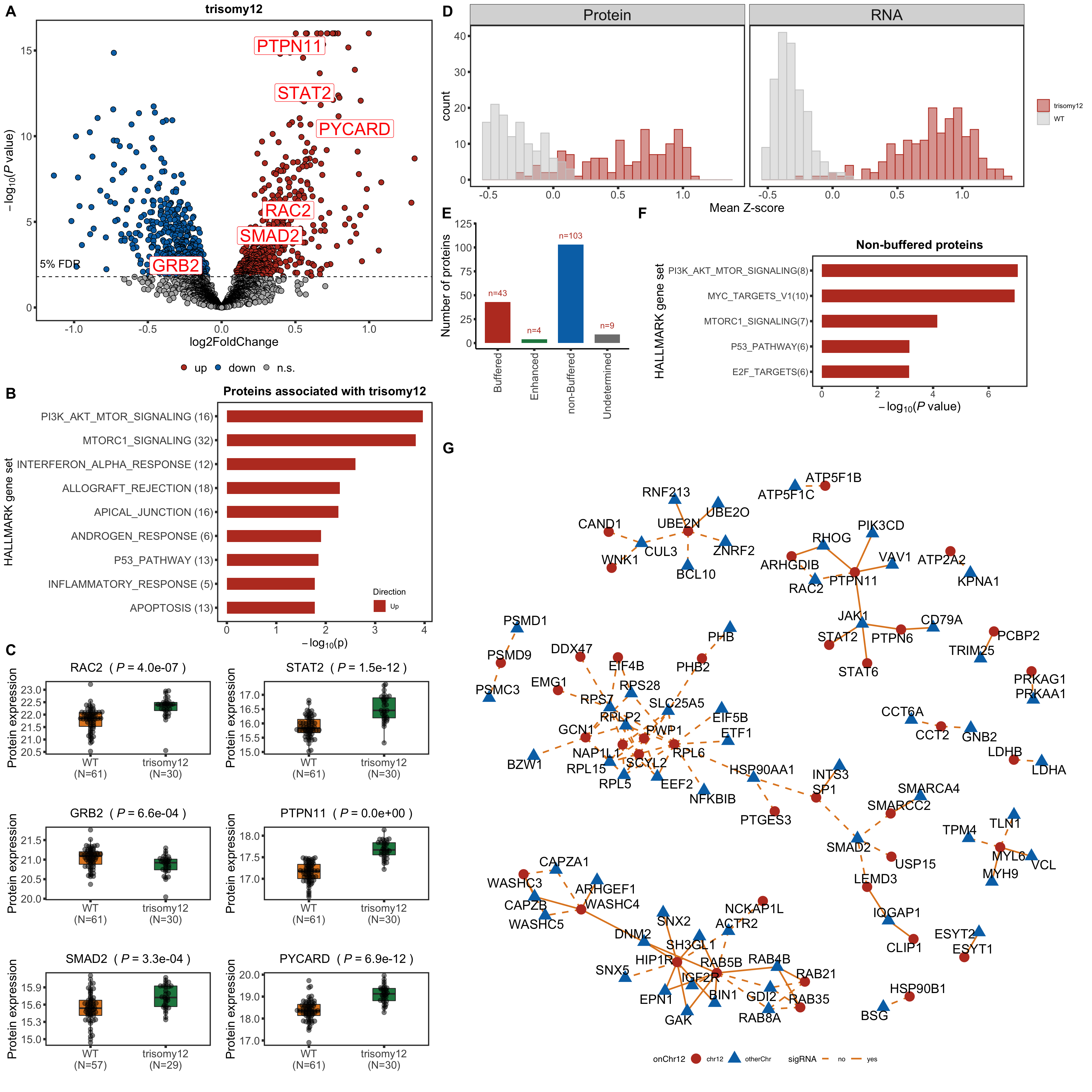
Protein abundance changes related to trisomy12
protRes <- resList %>% filter(Gene == "trisomy12") %>%
    mutate(Chr = rowData(protCLL[id,])$chromosome_name) %>%
    #filter(Chr == "12") %>%
    #mutate(adj.P.Val = p.adjust(P.Value, method= "BH")) %>%
    dplyr::rename(uniprotID = id,
                  pvalue = P.Value, padj = adj.P.global,
                  chrom = Chr) %>%
    mutate(geneID = rowData(protCLL[uniprotID,])$ensembl_gene_id) %>%
    select(name, uniprotID, geneID, chrom, log2FC, pvalue, padj, t) %>%
    dplyr::rename(stat =t) %>%
    arrange(pvalue) %>% as_tibble()
Combine
allRes <- left_join(protRes, rnaRes, by = "geneID") %>%
  filter(!is.na(stat), !is.na(stat.rna))
Only chr12 genes that are up-regulated are considered.
fdrCut <- 0.05

bufferTab <- allRes %>% filter(chrom %in% 12, stat.rna > 0, stat>0) %>%
  ungroup() %>%
  mutate(stat.prot.sqrt = sqrt(stat),
         stat.prot.center = stat.prot.sqrt - mean(stat.prot.sqrt,na.rm= TRUE)) %>%
  mutate(score = -stat.prot.center*stat.rna,
         diffFC = log2FC.rna-log2FC) %>%
  mutate(ifBuffer = case_when(
    padj < fdrCut & padj.rna < fdrCut & stat > 0 ~ "non-Buffered",
    padj > fdrCut & padj.rna < fdrCut ~ "Buffered",
    padj < fdrCut & padj.rna > fdrCut & stat > 0 ~ "Enhanced",
    TRUE ~ "Undetermined"
  )) %>%
  arrange(desc(score))
Table
bufferTab %>% select(name, geneID, chrom, ifBuffer, score, log2FC, padj, log2FC.rna, padj.rna) %>%
  mutate_if(is.numeric, formatC, digits=2) %>%
  DT::datatable()
Summary plot
sumTab <- bufferTab %>% group_by(ifBuffer) %>%
  summarise(n = length(name))

bufferPlot <- ggplot(sumTab, aes(x=ifBuffer, y = n)) +
  geom_bar(aes(fill = ifBuffer), stat="identity", width = 0.7) +
  geom_text(aes(label = paste0("n=", n)),vjust=-1,col=colList[1]) +
  scale_fill_manual(values =c(Buffered = colList[1],
                              Enhanced = colList[4],
                              `non-Buffered` = colList[2],
                              Undetermined = "grey50")) +
  theme_half + theme(axis.text.x = element_text(angle = 90, hjust=1, vjust=0.5),
                     legend.position = "none") +
  ylab("Number of proteins") + ylim(0,120) +xlab("")
bufferPlot

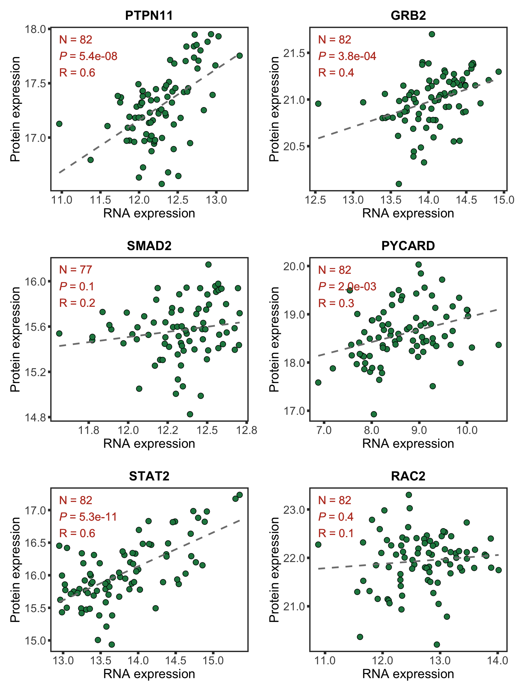
Plot example cases of buffered and non-buffered proteins
protList <- c("PTPN11","STAT2","CD27","SUDS3")
geneList <- bufferTab[match(protList, bufferTab$name),]$geneID
pList <- lapply(geneList, function(i) {
  tabProt <- protExprTab %>% filter(id == i) %>%
    select(id, patID,expr) %>% dplyr::rename(protExpr = expr)
  tabRna <- rnaExprTab %>% filter(id == i) %>%
    select(id, patID, expr) %>% dplyr::rename(rnaExpr = expr)
  plotTab <- left_join(tabProt, tabRna, by = c("id","patID")) %>%
    filter(!is.na(protExpr), !is.na(rnaExpr)) %>%
    mutate(trisomy12 = patMeta[match(patID, patMeta$Patient.ID),]$trisomy12) %>%
    mutate(trisomy12 = ifelse(trisomy12 %in% 1, "yes","no")) %>%
    mutate(symbol = rowData(dds[id,])$symbol)
  p <- ggplot(plotTab, aes(x=rnaExpr, y = protExpr)) +
    geom_point(aes(col=trisomy12)) +
    geom_smooth(formula =  y~x, method="lm",se=FALSE, color = "grey50", linetype ="dashed" ) +
    ggtitle(unique(plotTab$symbol)) +
    ylab("Protein expression") + xlab("RNA expression") +
    scale_color_manual(values =c(yes = colList[1],no=colList[2])) +
    theme_full + theme(legend.position = "bottom")
  ggExtra::ggMarginal(p, type = "histogram", groupFill = TRUE)
  })
cowplot::plot_grid(plotlist = pList, ncol=2)

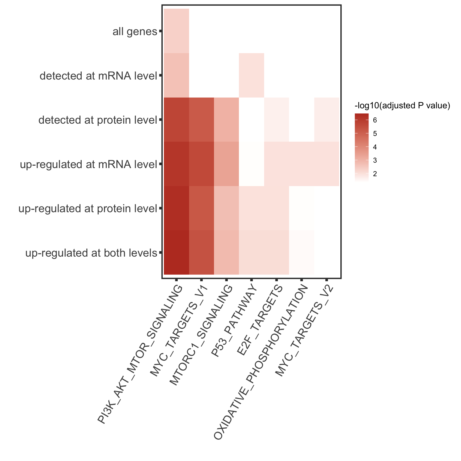
Enrichment of buffer and non-buffered proteins
Non-buffered prpteins
Using cancer hallmark genesets
rnaAll <- dds[rowData(dds)$biotype %in% "protein_coding" & !rowData(dds)$symbol %in% c("",NA),] #all protein coding gene as background

protList <- filter(bufferTab, ifBuffer == "non-Buffered")$name
refList <- rowData(rnaAll)$symbol
enRes <- runFisher(protList, refList, gmts$H, pCut =0.01, ifFDR = TRUE,removePrefix = "HALLMARK_",
                   plotTitle = "Non-buffered proteins", insideLegend = TRUE,
                   setName = "HALLMARK gene set")
bufferEnrich <- enRes$enrichPlot + theme(plot.margin = margin(1,3,1,1, unit = "cm"))
bufferEnrich

Buffered proteins
protList <- filter(bufferTab, ifBuffer == "Buffered")$name
enRes <- runFisher(protList, refList, gmts$H, pCut =0.1, ifFDR = TRUE)
[1] "No sets passed the criteria"
No enrichment
Compare buffering effect between trisomy19 and trisomy12
load("../output/deResList.RData")
load("../output/deResListRNA.RData")
testTabProt <- resList %>% mutate(chr = rowData(protCLL[id,])$chromosome_name) %>%
  filter(Gene == paste0("trisomy",chr)) %>%
  select(name, log2FC, Gene) %>% mutate(type = "Protein")
testTabRNA <- resListRNA %>% mutate(chr = rowData(dds[id,])$chromosome) %>%
  filter(Gene == paste0("trisomy",chr)) %>%
  select(name, log2FC, Gene) %>% mutate(type = "RNA")
overGene <- intersect(testTabProt$name, testTabRNA$name)
testTab <- bind_rows(testTabProt, testTabRNA) %>%
  filter(name %in% overGene)
plotTab <- lapply(seq(-2,2, length.out = 50), function(foldCut) {
  filTab <- mutate(testTab, pass = log2FC > foldCut) %>%
    group_by(Gene, type) %>% summarise(n = sum(pass),per = sum(pass)/length(pass)) %>%
    mutate(cut = foldCut)
}) %>% bind_rows() %>%
  mutate(group =paste0(Gene,"_",type))
Cummulative plot
ggplot(plotTab, aes(x=cut, y = per))+
  geom_line(aes(col = Gene, linetype = type),size=1) +
  scale_color_manual(values = c(trisomy12 = colList[1],trisomy19=colList[2]), name = "") +
  scale_linetype_discrete(name = "") +
  coord_cartesian(xlim=c(1.5,-1)) +
  ylab("Cumulative fraction") +
  xlab("log2 (fold change)") +
  theme_full +
  theme(legend.position = c(0.8,0.3))

KS test
RNA level
testTab <- plotTab %>% filter(type == "RNA") %>%
  select(Gene, per,cut) %>% pivot_wider(names_from = Gene, values_from = per)
ks.test(testTab$trisomy12, testTab$trisomy19)
    Two-sample Kolmogorov-Smirnov test

data:  testTab$trisomy12 and testTab$trisomy19
D = 0.24, p-value = 0.1122
alternative hypothesis: two-sided
Protein level
testTab <- plotTab %>% filter(type == "Protein") %>%
  select(Gene, per,cut) %>% pivot_wider(names_from = Gene, values_from = per)
ks.test(testTab$trisomy12, testTab$trisomy19)
    Two-sample Kolmogorov-Smirnov test

data:  testTab$trisomy12 and testTab$trisomy19
D = 0.42, p-value = 0.0002955
alternative hypothesis: two-sided
Plot expression on genomic coordiate
patBack <- dplyr::filter(patMeta, Patient.ID %in% unique(allProtTab$patID)) %>%
  dplyr::select(Patient.ID, trisomy12) %>%
  dplyr::rename(patID = Patient.ID) %>%
  mutate_all(as.character) %>%
  mutate_at(vars(-patID),str_replace, "1","yes") %>%
  mutate_at(vars(-patID),str_replace, "0","no")
plotExprVar <- function(gene, chr, patBack, allBand, allLine, allProtTab, allRnaTab, protLine = NULL,
                        region = c(-Inf,Inf),ifTrend = FALSE, normalize = TRUE, maxVal =2, minVal=-2) {

  #table for cyto band
  bandTab <- filter(allBand, ChromID == chr, chromStart >= region[1], chromEnd <= region[2]) %>%
    mutate(chromMid = chromMid)

  #table for expression
  plotProtTab <- filter(allProtTab, ChromID == chr, start_position >= region[1], end_position <= region[2]) %>%
    mutate_if(is.factor,as.character)
  plotRnaTab <- filter(allRnaTab, ChromID == chr, start_position >= region[1], end_position <= region[2]) %>%
    mutate_if(is.factor,as.character)


  #summarise group mean
  plotProtTab <- plotProtTab %>%
    mutate(group = patBack[match(patID, patBack$patID),][[gene]]) %>%
    filter(!is.na(group)) %>%
    group_by(id, group) %>% mutate(meanExpr = mean(expr, na.rm=TRUE)) %>%
    distinct(group, id,.keep_all = TRUE) %>% ungroup()

  plotRnaTab <- plotRnaTab %>%
    mutate(group = patBack[match(patID, patBack$patID),][[gene]]) %>%
    filter(!is.na(group)) %>%
    group_by(id, group) %>% mutate(meanExpr = mean(expr, na.rm=TRUE)) %>%
    distinct(group, id,.keep_all = TRUE) %>% ungroup()

  if (!is.null(protLine)) {
    bufferLineTab <- plotProtTab %>%
      select(symbol, mid_position, meanExpr, group) %>%
      filter(symbol %in% protLine) %>%
      pivot_wider(names_from = group, values_from = meanExpr) %>%
      mutate(lowVal = map2_dbl(yes, no, min),
             highVal = map2_dbl(yes, no, max))
  } else bufferLineTab <- NULL


  xMax <- max(bandTab$chromEnd, na.rm = T)

  #main plot for Protein
  gPro <- ggplot() +
    geom_rect(data=bandTab, mapping=aes(xmin=chromStart, xmax=chromEnd, ymin=minVal+0.5, ymax=maxVal-0.5,
                                        fill=Colour, label = band), alpha=0.1) +
    geom_text(data=bandTab, mapping=aes(label=band, x=chromMid), y=maxVal-0.5, hjust =1, angle = 90, size=2.5)

  if (!is.null(protLine)) {
    gPro <- gPro + geom_segment(data = bufferLineTab, aes(x=mid_position, xend = mid_position,
                                        y=lowVal, yend = highVal), linetype = "dashed")

  }

  gPro <- gPro + geom_rect(data = plotProtTab,
            mapping=aes(xmin=start_position,
                        xmax=end_position, ymin=meanExpr, ymax=meanExpr+0.1,
                        fill = group, label = symbol)) +
    scale_x_continuous(expand=c(0,0),limits = c(0,xMax)) +
    xlab("Genomic position [Mb]") +
    ylab("Expression (normalized by length)") +
    scale_fill_manual(values = c(even = "white",odd = "grey50",
                                yes = "darkred", no = "darkgreen")) +
    scale_color_manual(values = c(yes = "darkred",no = "darkgreen")) +
    ggtitle(paste0("Protein expression","(",chr,")")) +
    theme(plot.title = element_text(face = "bold", size = 10),
        legend.position = "none",
        panel.background = element_blank(),
        panel.grid.major = element_line(colour="grey90", size=0.1))

    if (ifTrend) {
      gPro <- gPro + geom_smooth(data =filter(plotProtTab, expr >0),
                mapping = aes(y=meanExpr, x= mid_position,
                              color = group),
                formula = y ~ x, method = "loess", se=FALSE, span=0.5,
                size =0.2, alpha=0.5)
    }

  #main plot for RNA
  gRna <- ggplot() +
    geom_rect(data=bandTab, mapping=aes(xmin=chromStart, xmax=chromEnd, ymin=minVal, ymax=maxVal,
                                        fill=Colour, label = band), alpha=0.1) +
    geom_text(data=bandTab, mapping=aes(label=band, x=chromMid), y=maxVal, hjust =1, angle = 90, size=2.5) +
    geom_rect(data = plotRnaTab,
            mapping=aes(xmin=start_position,
                        xmax=end_position, ymin=meanExpr, ymax=meanExpr+0.1,
                        fill = group, label = symbol)) +
    scale_x_continuous(expand=c(0,0),limits = c(0,xMax)) +
    xlab("Genomic position [Mb]") +
    ylab("Expression Z-score") +
    scale_fill_manual(values = c(even = "white",odd = "grey50",
                                yes = "darkred", no = "darkgreen")) +
    scale_color_manual(values = c(yes = "darkred", no = "darkgreen")) +
    ggtitle(paste0("RNA expression","(",chr,")")) +
    theme(plot.title = element_text(face = "bold", size = 10),
        legend.position = "none",
        panel.background = element_blank(),
        panel.grid.major = element_line(colour="grey90", size=0.1))

    if (ifTrend) {
      gRna <- gRna + geom_smooth(data =filter(plotRnaTab),
                mapping = aes(y=meanExpr, x= mid_position,
                              color = group),
                formula = y ~ x, method = "loess", se=FALSE, span=0.2,
                size =0.2, alpha=0.5)
    }
    #for legend
    ## if the patient has CNV data
    lgTab <- tibble(x= seq(6),y=seq(6),
                    Expression = c(rep("yes",3), rep("no",3)))

    lg <- ggplot(lgTab, aes(x=x,y=y)) +
        geom_point(aes(fill = Expression), shape =22,size=3) +
        scale_fill_manual(values = c(yes = "darkred", no = "darkgreen"), name = gene) +
        theme(legend.position = "bottom")

    lg <- get_legend(lg)

    return(list(plotPro = gPro, plotRNA = gRna, legend = lg))
}
Normalize protein and RNA expression
normalized <- TRUE
#if perform normalization
if (normalized) {
  #for protein
  exprMat <- select(allProtTab,patID, id,expr) %>%
    distinct(patID, id, .keep_all = TRUE) %>%
    spread(key = patID, value =expr) %>% data.frame() %>%
    column_to_rownames("id") %>% as.matrix()
  qm <- jyluMisc::mscale(exprMat, useMad = F)
  normTab <- data.frame(qm) %>% rownames_to_column("id") %>%
    gather(key = "patID", value = "expr", -id)
  allProtTab <- select(allProtTab, -expr) %>% left_join(normTab, by = c("patID","id"))


  #for RNA
  exprMat <- select(allRnaTab,patID, id,expr) %>%
    distinct(patID, id, .keep_all = TRUE) %>%
    spread(key = patID, value =expr) %>% data.frame() %>%
    column_to_rownames("id") %>% as.matrix()
  qm <- jyluMisc::mscale(exprMat, useMad = F)
  normTab <- data.frame(qm) %>% rownames_to_column("id") %>%
    gather(key = "patID", value = "expr", -id)
  allRnaTab <- select(allRnaTab, -expr) %>% left_join(normTab, by = c("patID","id"))
}
g <- plotExprVar("trisomy12","chr12",patBack,allBand, allLine,
                 allProtTab, allRnaTab, ifTrend = TRUE)
plot_grid(g$plotRNA, g$plotPro, g$legend, ncol = 1, rel_heights = c(1,1,0.2))


 PLCG1 is not significant anymore


 ### PCA