Overview of differentially expressed proteins
A table of associations with 5% FDR
resList <- filter(resList, Gene == "trisomy19") %>%
  #mutate(adj.P.Val = adj.P.global) %>% #use IHW corrected P-value
  mutate(Chr = rowData(protCLL[id,])$chromosome_name)
resList %>% filter(adj.P.Val <= 0.05) %>%
  select(name, Chr,logFC, P.Value, adj.P.Val) %>%
  mutate_if(is.numeric, formatC, digits=2) %>%
  DT::datatable()
Heatmap of differentially expressed proteins (5% FDR)
(Restricted to M-CLL with trisomy12)
protCLL$IGHV.status <- patMeta[match(colnames(protCLL),patMeta$Patient.ID),]$IGHV.status
protCLL$trisomy12 <- patMeta[match(colnames(protCLL),patMeta$Patient.ID),]$trisomy12

proList <- filter(resList, !is.na(name), adj.P.Val < 0.05) %>%
  arrange(desc(t)) %>%
  distinct(name, .keep_all = TRUE) %>% pull(id)
plotMat <- assays(protCLL)[["QRILC_combat"]][proList, protCLL$IGHV.status %in% "M" & protCLL$trisomy12 %in% 1]
rownames(plotMat) <- rowData(protCLL[proList,])$hgnc_symbol

colAnno <- filter(patMeta, Patient.ID %in% colnames(protCLL)) %>%
  select(Patient.ID, trisomy12, IGHV.status,trisomy19) %>%
  data.frame() %>% column_to_rownames("Patient.ID")
colAnno$trisomy12 <- ifelse(colAnno$trisomy12 %in% 1, "yes","no")
colAnno$trisomy19 <- ifelse(colAnno$trisomy19 %in% 1, "yes","no")

rowAnno <- rowData(protCLL)[proList,c("chromosome_name","hgnc_symbol"),drop=FALSE] %>%
  data.frame(stringsAsFactors = FALSE) %>%
  mutate(onChr19 = ifelse(chromosome_name == "19","yes","no")) %>%
  select(hgnc_symbol, onChr19) %>% data.frame() %>% remove_rownames() %>%
  column_to_rownames("hgnc_symbol")

plotMat <- jyluMisc::mscale(plotMat, censor = 5)

annoCol <- list(trisomy12 = c(yes = "black",no = "grey80"),
                trisomy19 = c(yes = "black",no = "grey80"),
                IGHV.status = c(M = colList[3], U = colList[4]),
                onChr19 = c(yes = colList[1],no = "white"))

tri19Heatmap <- pheatmap::pheatmap(plotMat, annotation_col = colAnno, scale = "none",
                   annotation_row = rowAnno,
                   cluster_rows = FALSE,
                   clustering_method = "ward.D2",
                   color = colorRampPalette(c(colList[2],"white",colList[1]))(100),
                   breaks = seq(-5,5, length.out = 101), annotation_colors = annoCol,
                   show_rownames = TRUE, show_colnames = FALSE,
                   treeheight_row = 0, silent = TRUE)$gtable
plot_grid(tri19Heatmap)

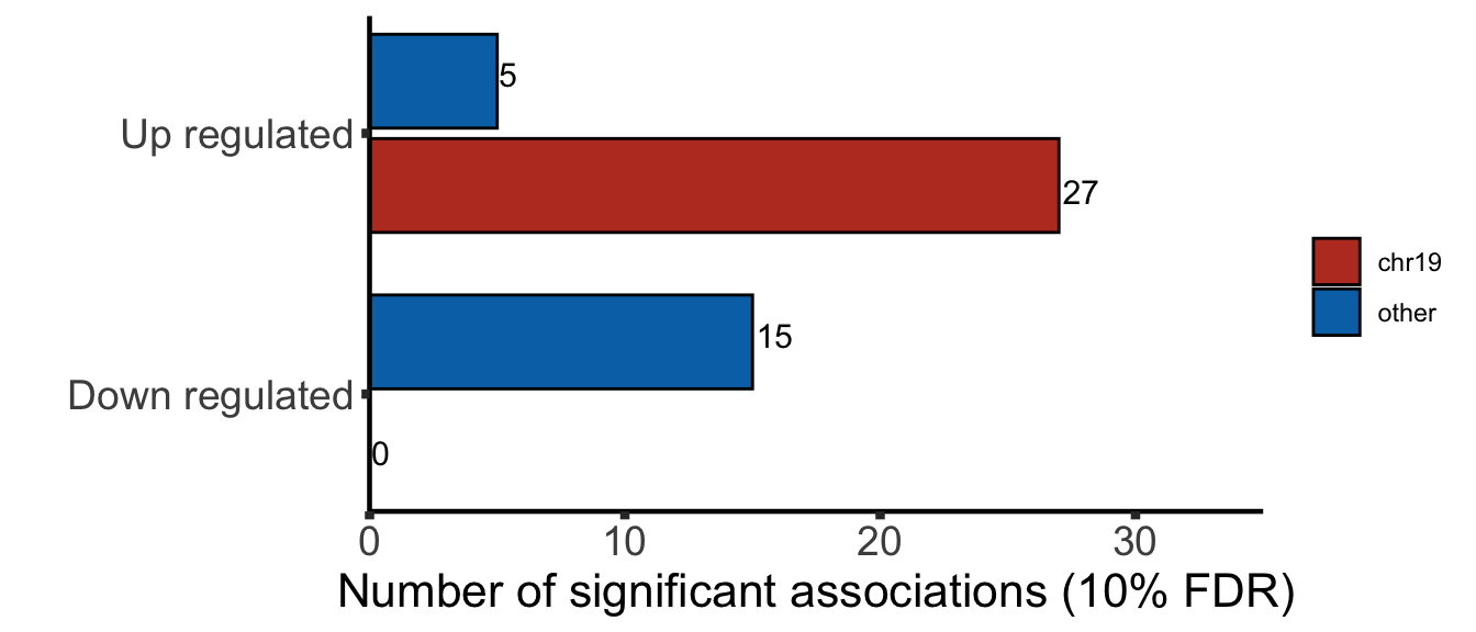
Summary of chromosome distribution (5% FDR)
plotTab <- filter(resList, adj.P.Val <=0.05) %>% mutate(change = ifelse(logFC>0,"Up regulated","Down regulated"),
                              chromosome = ifelse(Chr %in% "19","chr19","other")) %>%
  group_by(change, chromosome) %>% summarise(n = length(id)) %>%
  bind_rows(tibble(change = "Down regulated", chromosome = "chr19",  n =0))

sigNumPlot <- ggplot(plotTab, aes(x=change, y=n, fill = chromosome)) +
  geom_bar(stat = "identity", width = 0.8,
           position = position_dodge2(width = 6),
           col = "black") +
  geom_text(aes(label=n),
            position = position_dodge(width = 0.9),
            size=4, hjust=-0.1)  +
  scale_fill_manual(name = "", labels = c("chr19","other"), values = colList) +
  coord_flip(ylim = c(0,35), expand = FALSE) + xlab("") + ylab("Number of significant associations (10% FDR)") + theme_half
sigNumPlot
 ## Enrichment analysis
Barplot of enriched pathways
gmts = list(H= "../data/gmts/h.all.v6.2.symbols.gmt",
            KEGG = "../data/gmts/c2.cp.kegg.v6.2.symbols.gmt",
            GO = "../data/gmts/c5.bp.v6.2.symbols.gmt")
inputTab <- resList %>% filter(P.Value < 0.05) %>%
  mutate(name = rowData(protCLL[id,])$hgnc_symbol) %>% filter(!is.na(name)) %>%
  distinct(name, .keep_all = TRUE) %>%
  select(name, t) %>% data.frame() %>% column_to_rownames("name")
enRes <- list()
enRes[["Proteins associated with trisomy19"]] <- runGSEA(inputTab, gmts$H, "page")

p <- plotEnrichmentBar(enRes[[1]], pCut =0.05, ifFDR= FALSE, setName = "HALLMARK gene set",
                       title = names(enRes)[1], removePrefix = "HALLMARK_", insideLegend=TRUE)
tri19Enrich <- cowplot::plot_grid(p)
tri19Enrich

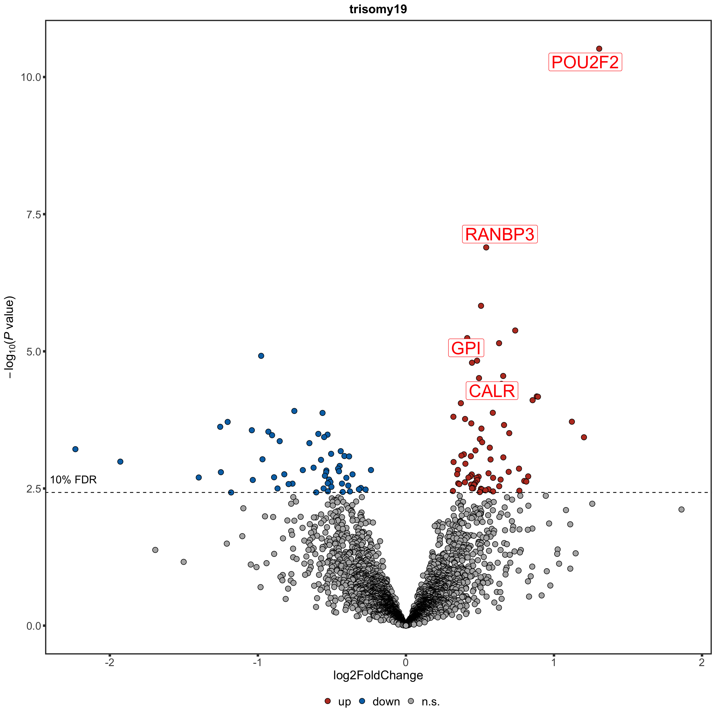
Volcano plot
plotTab <- resList %>% mutate(onChr19 = ifelse(Chr %in% "19","yes","no"))
#nameList <- filter(resList, adj.P.Val <=0.1)$name
nameList <- c("GPI","CALR","RRAS","RANBP3","EIF4EBP1","POU2F2")
tri19Volcano <- plotVolcano(plotTab, fdrCut =0.1, x_lab="log2FoldChange", posCol = colList[1], negCol = colList[2],
            plotTitle = "trisomy19", ifLabel = TRUE, labelList = nameList)
tri19Volcano
New list of detected candiates
nameList <- c("GPI","RANBP3","CALR","POU2F2")
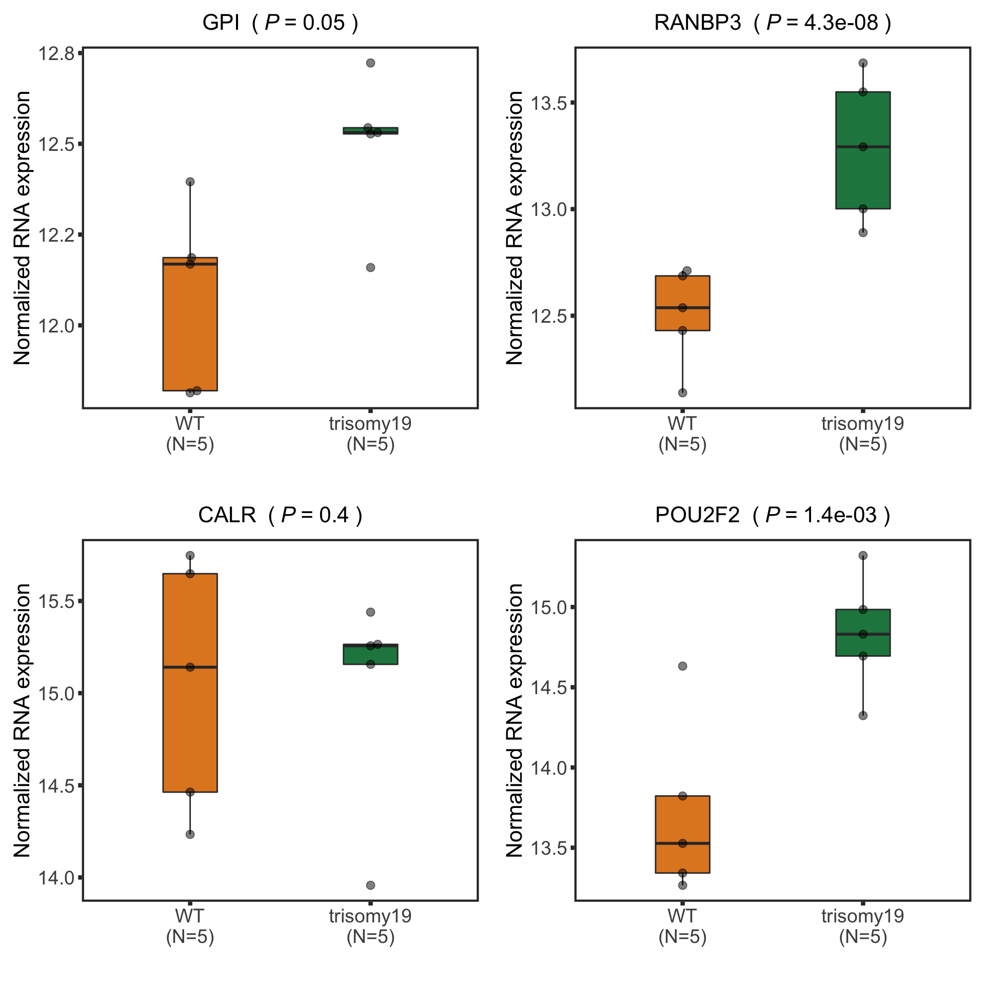
Boxplot plot of selected genes (top 10 most differentially expressed)
(Restricted to M-CLL with trisomy19)
protSub <- protCLL[, protCLL$IGHV.status %in% "M" & protCLL$trisomy12 %in% 1]

protTab <- sumToTidy(protSub, rowID = "uniprotID", colID = "patID")
resList.sig <- filter(resList, adj.P.Val < 0.1)
#nameList <- resList.sig$name[1:10]
plotTab <- protTab %>% filter(hgnc_symbol %in% nameList) %>%
  mutate(trisomy19 = patMeta[match(patID, patMeta$Patient.ID),]$trisomy19) %>%
  mutate(status = ifelse(trisomy19 %in% 1,"trisomy19","WT"),
         name = hgnc_symbol) %>%
  mutate(status=factor(status, levels = c("WT","trisomy19")))
pList <- plotBox(plotTab, pValTabel = resList, y_lab = "Protein expression")
tri19Box<-cowplot::plot_grid(plotlist= pList, ncol=2)
tri19Box
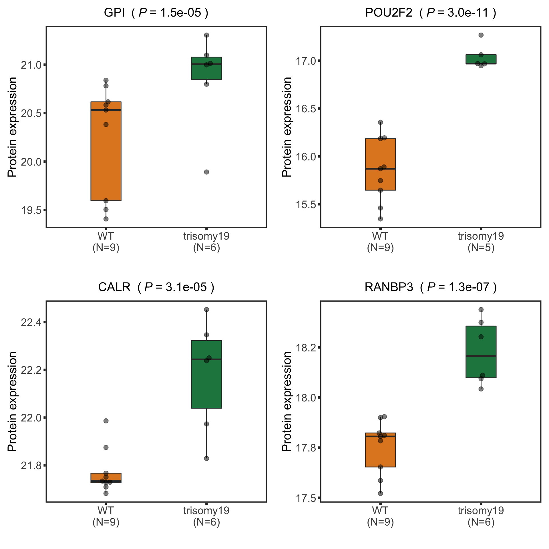 Some candidates are not detected anymore. # Compare with RNA sequencing data
Buffering of gene dosage effect
Visualizing gene dosage effect on protein and RNA level
Log2 protein counts
protExprTab <- sumToTidy(protCLL) %>%
  filter(chromosome_name == "19") %>%
  mutate(id = ensembl_gene_id, patID = colID, expr = log2Norm_combat, type = "Protein") %>%
  select(id, patID, expr, type)
Log2 RNA seq counts
rnaExprTab <- counts(dds[rownames(dds) %in% protExprTab$id,
                            colnames(dds) %in% protExprTab$patID], normalized= TRUE) %>%
  as_tibble(rownames = "id") %>%
  pivot_longer(-id, names_to = "patID", values_to = "count") %>%
  mutate(expr = log2(count)) %>%
  select(id, patID, expr) %>% mutate(type = "RNA")
comExprTab <- bind_rows(rnaExprTab, protExprTab) %>%
  mutate(trisomy12 = patMeta[match(patID, patMeta$Patient.ID),]$trisomy12) %>%
  filter(!is.na(trisomy12)) %>% mutate(cnv = ifelse(trisomy12 %in% 1, "trisomy12","WT"))
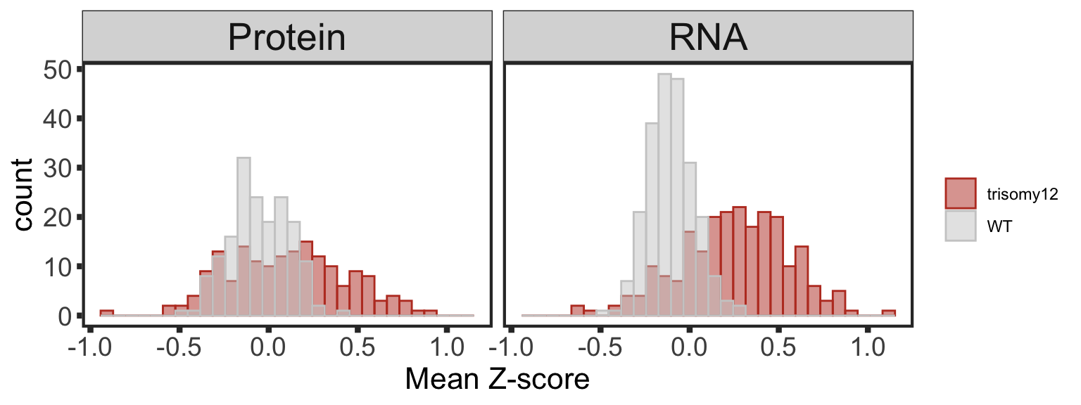
In the plots below, the RNAseq dataset is subsetted for genes that also present in proteomic dataset. The plots will look somewhat different in all genes are used. But the trend is the same
Proteins/RNAs on Chr19 have higher expressions in trisomy19 samples compared to other samples
plotTab <- comExprTab %>%
  group_by(id,type) %>% mutate(zscore = (expr-mean(expr))/sd(expr)) %>%
  group_by(id, cnv, type) %>% summarise(meanExpr = mean(zscore, na.rm=TRUE)) %>%
  ungroup()

dosagePlot <- ggplot(plotTab, aes(x=meanExpr, fill = cnv, col=cnv)) +
  geom_histogram(position = "identity", alpha=0.5, bins=30) + facet_wrap(~type, scale = "fixed") +
  scale_fill_manual(values = c(WT = "grey80", trisomy12 = colList[1]), name = "") +
  scale_color_manual(values = c(WT = "grey80", trisomy12 = colList[1]), name = "") +
  #xlim(-1,1) +
  theme_full + xlab("Mean Z-score") +
  theme(strip.text = element_text(size =20))

dosagePlot
Analyzing buffering effect
Detect buffered and non-buffered proteins
Preprocessing protein and RNA data
#subset samples and genes
overSampe <- intersect(colnames(ddsCLL), colnames(protCLL))
overGene <- intersect(rownames(ddsCLL), rowData(protCLL)$ensembl_gene_id)
ddsSub <- ddsCLL[overGene, overSampe]
protSub <- protCLL[match(overGene, rowData(protCLL)$ensembl_gene_id),overSampe]
rowData(ddsSub)$uniprotID <- rownames(protSub)[match(rownames(ddsSub),rowData(protSub)$ensembl_gene_id)]

#vst
ddsSub.vst <- varianceStabilizingTransformation(ddsSub)
Differential expression on RNA level
rnaRes <- resListRNA %>% filter(Gene == "trisomy19") %>%
  mutate(Chr = rowData(dds[id,])$chromosome) %>%
  #filter(Chr == "12") %>%
  #mutate(adj.P.Val = p.adjust(P.Value, method = "BH")) %>%
  dplyr::rename(geneID = id, log2FC.rna = log2FC,
                pvalue.rna = P.Value, padj.rna = adj.P.Val, stat.rna= t) %>%
  select(geneID, log2FC.rna, pvalue.rna, padj.rna, stat.rna)
Protein abundance changes related to trisomy19
fdrCut <- 0.05
protRes <- resList %>% filter(Gene == "trisomy19") %>%
    dplyr::rename(uniprotID = id,
                  pvalue = P.Value, padj = adj.P.global,
                  chrom = Chr) %>%
    mutate(geneID = rowData(protCLL[uniprotID,])$ensembl_gene_id) %>%
    select(name, uniprotID, geneID, chrom, log2FC, pvalue, padj, t) %>%
    dplyr::rename(stat =t) %>%
    arrange(pvalue) %>% as_tibble()
Combine
allRes <- left_join(protRes, rnaRes, by = "geneID")
Only chr19 genes that are up-regulated are considered.
bufferTab <- allRes %>% filter(chrom %in% 19,stat.rna > 0, stat>0) %>%
  ungroup() %>%
  mutate(stat.prot.sqrt = sqrt(stat),
         stat.prot.center = stat.prot.sqrt - mean(stat.prot.sqrt, na.rm = TRUE)) %>%
  mutate(score = -stat.prot.center*stat.rna,
         diffFC = log2FC.rna - log2FC) %>%
  mutate(ifBuffer = case_when(
    padj < fdrCut & padj.rna < fdrCut & stat > 0 ~ "non-Buffered",
    padj > fdrCut & padj.rna < fdrCut ~ "Buffered",
    padj < fdrCut & padj.rna > fdrCut & stat > 0 ~ "Enhanced",
    TRUE ~ "Undetermined"
  )) %>%
  arrange(desc(score))
Table of buffering status
bufferTab %>% mutate_if(is.numeric, formatC, digits=2) %>%
  select(name, pvalue, pvalue.rna, padj, padj.rna, ifBuffer) %>%
  DT::datatable()
Summary plot
sumTab <- bufferTab %>% group_by(ifBuffer) %>%
  summarise(n = length(name))

bufferPlot <- ggplot(sumTab, aes(x=ifBuffer, y = n)) +
  geom_bar(aes(fill = ifBuffer), stat="identity", width = 0.7) +
  geom_text(aes(label = paste0("n=", n)),vjust=-1,col=colList[1]) +
  scale_fill_manual(values =c(Buffered = colList[1],
                              Enhanced = colList[4],
                              `non-Buffered` = colList[2],
                              Undetermined = "grey50")) +
  theme_half + theme(axis.text.x = element_text(angle = 90, hjust=1, vjust=0.5),
                     legend.position = "none") +
  ylab("Number of proteins") + ylim(0,130) +xlab("")
bufferPlot

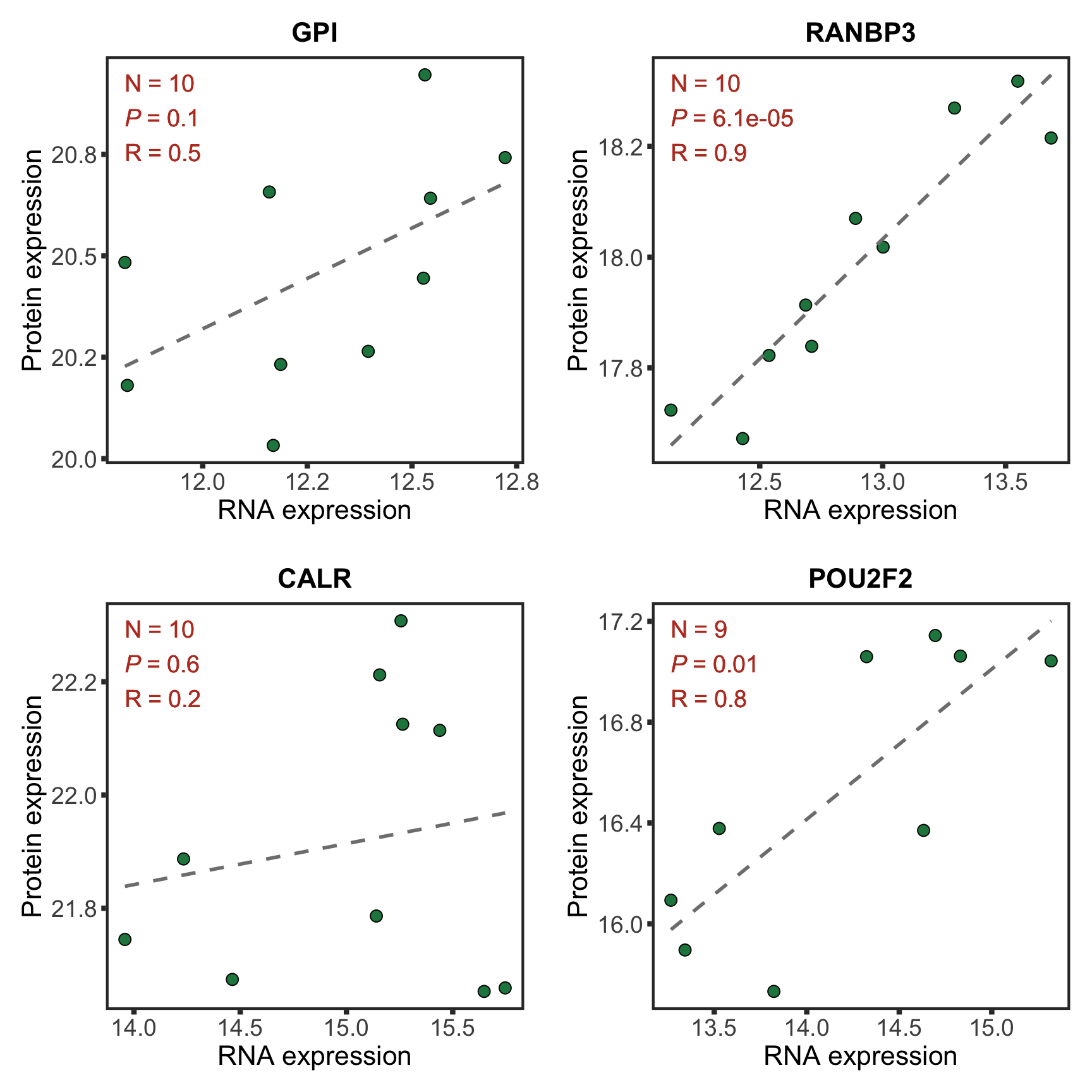
Plot example cases of buffered and non-buffered proteins
protList <- c("POU2F2","RANBP3","CD79A", "MAP4K1")
geneList <- bufferTab[match(protList, bufferTab$name),]$geneID
pList <- lapply(geneList, function(i) {
  tabProt <- allProtTab %>% filter(id == i) %>%
    select(id, patID, symbol,expr) %>% dplyr::rename(protExpr = expr)
  tabRna <- allRnaTab %>% filter(id == i) %>%
    select(id, patID, expr) %>% dplyr::rename(rnaExpr = expr)
  plotTab <- left_join(tabProt, tabRna, by = c("id","patID")) %>%
    filter(!is.na(protExpr), !is.na(rnaExpr)) %>%
    mutate(trisomy19 = patMeta[match(patID, patMeta$Patient.ID),]$trisomy19,
           trisomy12 = patMeta[match(patID, patMeta$Patient.ID),]$trisomy12,
           IGHV = patMeta[match(patID, patMeta$Patient.ID),]$IGHV.status) %>%
    filter(!is.na(trisomy19),trisomy12 %in% 1, IGHV %in%"M") %>%
    mutate(trisomy19 = ifelse(trisomy19 %in% 1, "yes","no"))
  p <- ggplot(plotTab, aes(x=rnaExpr, y = protExpr)) +
    geom_point(aes(col=trisomy19)) +
    geom_smooth(formula =  y~x, method="lm",se=FALSE, color = "grey50", linetype ="dashed" ) +
    ggtitle(unique(plotTab$symbol)) +
    ylab("Protein expression") + xlab("RNA expression") +
    scale_color_manual(values =c(yes = colList[1],no=colList[2])) +
    theme_full + theme(legend.position = "bottom")
  ggExtra::ggMarginal(p, type = "histogram", groupFill = TRUE)
  })
cowplot::plot_grid(plotlist = pList, ncol=2)
Enrichment of buffer and non-buffered proteins
Non-buffered prpteins
Using cancer hallmark genesets
protList <- filter(bufferTab, ifBuffer == "non-Buffered")$name
refList <- unique(protExprTab$symbol)
enRes <- runFisher(protList, refList, gmts$H, pCut =0.1, ifFDR = TRUE,removePrefix = "HALLMARK_",
                   plotTitle = "Non-buffered proteins", insideLegend = TRUE,
                   setName = "HALLMARK gene set")
[1] "No sets passed the criteria"
bufferEnrich <- enRes$enrichPlot + theme(plot.margin = margin(1,3,1,1, unit = "cm"))
bufferEnrich
NULL
Using GO Biological Process gene sets
protList <- filter(bufferTab, ifBuffer == "non-Buffered")$name
refList <- unique(protExprTab$symbol)
enRes <- runFisher(protList, refList, gmts$GO, pCut =0.1, ifFDR = TRUE,removePrefix = "GO_",
                   plotTitle = "Non-buffered proteins", insideLegend = TRUE,
                   setName = "GO BP gene set")
[1] "No sets passed the criteria"
bufferEnrich <- enRes$enrichPlot + theme(plot.margin = margin(1,3,1,1, unit = "cm"))
bufferEnrich
NULL
Buffered proteins
protList <- filter(bufferTab, ifBuffer == "Buffered")$name
enRes <- runFisher(protList, refList, gmts$H, pCut =0.1, ifFDR = TRUE)
[1] "No sets passed the criteria"
No enrichment
Compare buffer score and wehther protiens are in complexes
int_pairs <- read_csv2("../output/int_pairs.csv")


testTab <- bufferTab %>% mutate(inComplex = ifelse(uniprotID %in% c(int_pairs$ProtA,int_pairs$ProtB),
                                                   "complex in","complex out"))
tRes <- t.test(diffFC~inComplex, testTab)

ggplot(testTab, aes(x=inComplex, y=diffFC)) +
  geom_boxplot(outlier.shape = NA) + ggbeeswarm::geom_quasirandom() + theme_full +
  xlab("") + ylab("log2(RNA fold change) - log2(protein fold change)") +
  annotate("text", label = sprintf("P = %s",formatC(tRes$p.value, digits = 2)), x=Inf, y=Inf, hjust=2, vjust=3) +
  ylim(-0.5,1.5)
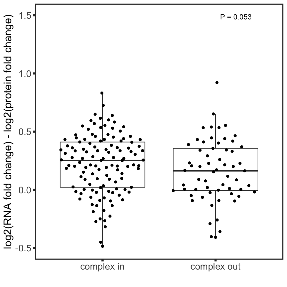 There’s no association between buffering status and whether the protein is in complex or not.