Preprocessing
Preprocessing protein and RNA data
#subset samples and genes
overSampe <- intersect(colnames(ddsCLL), colnames(protCLL))
overGene <- intersect(rownames(ddsCLL), rowData(protCLL)$ensembl_gene_id)
ddsSub <- ddsCLL[overGene, overSampe]
protSub <- protCLL[match(overGene, rowData(protCLL)$ensembl_gene_id),overSampe]
rowData(ddsSub)$uniprotID <- rownames(protSub)[match(rownames(ddsSub),rowData(protSub)$ensembl_gene_id)]

#vst
ddsSub.vst <- varianceStabilizingTransformation(ddsSub)
Processing protein complex data
int_pairs <- int_pairs <- read_csv2("../output/int_pairs.csv")
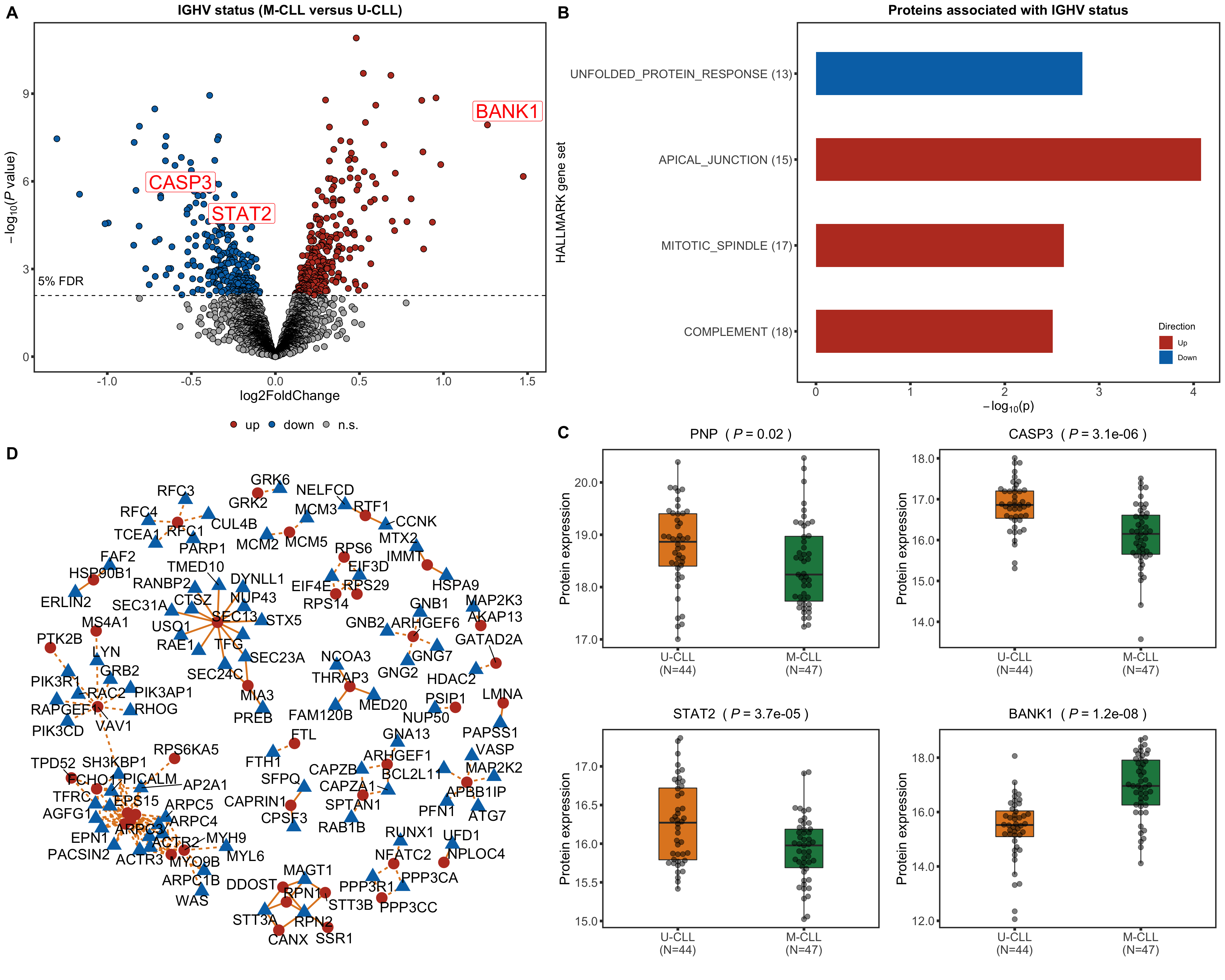
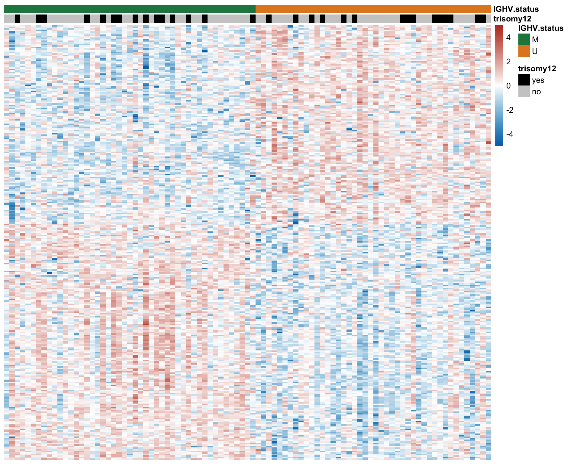
Differential RNA/protein expression analysis related to IGHV
Differential expression on RNA level
#design(ddsSub) <- ~ trisomy12 + IGHV
#deRes <- DESeq(ddsSub, betaPrior = TRUE)
rnaRes <- resListRNA %>% filter(Gene == "IGHV.status") %>%
  mutate(Chr = rowData(dds[id,])$chromosome) %>%
  #filter(Chr == "12") %>%
  #mutate(adj.P.Val = p.adjust(P.Value, method = "BH")) %>%
  dplyr::rename(geneID = id, log2FC.rna = log2FC,
                pvalue.rna = P.Value, padj.rna = adj.P.Val, stat.rna= t) %>%
  select(geneID, log2FC.rna, pvalue.rna, padj.rna, stat.rna)
Number of differentially expressed RNA (10% FDR)
nrow(filter(rnaRes, padj.rna <0.05))
[1] 386
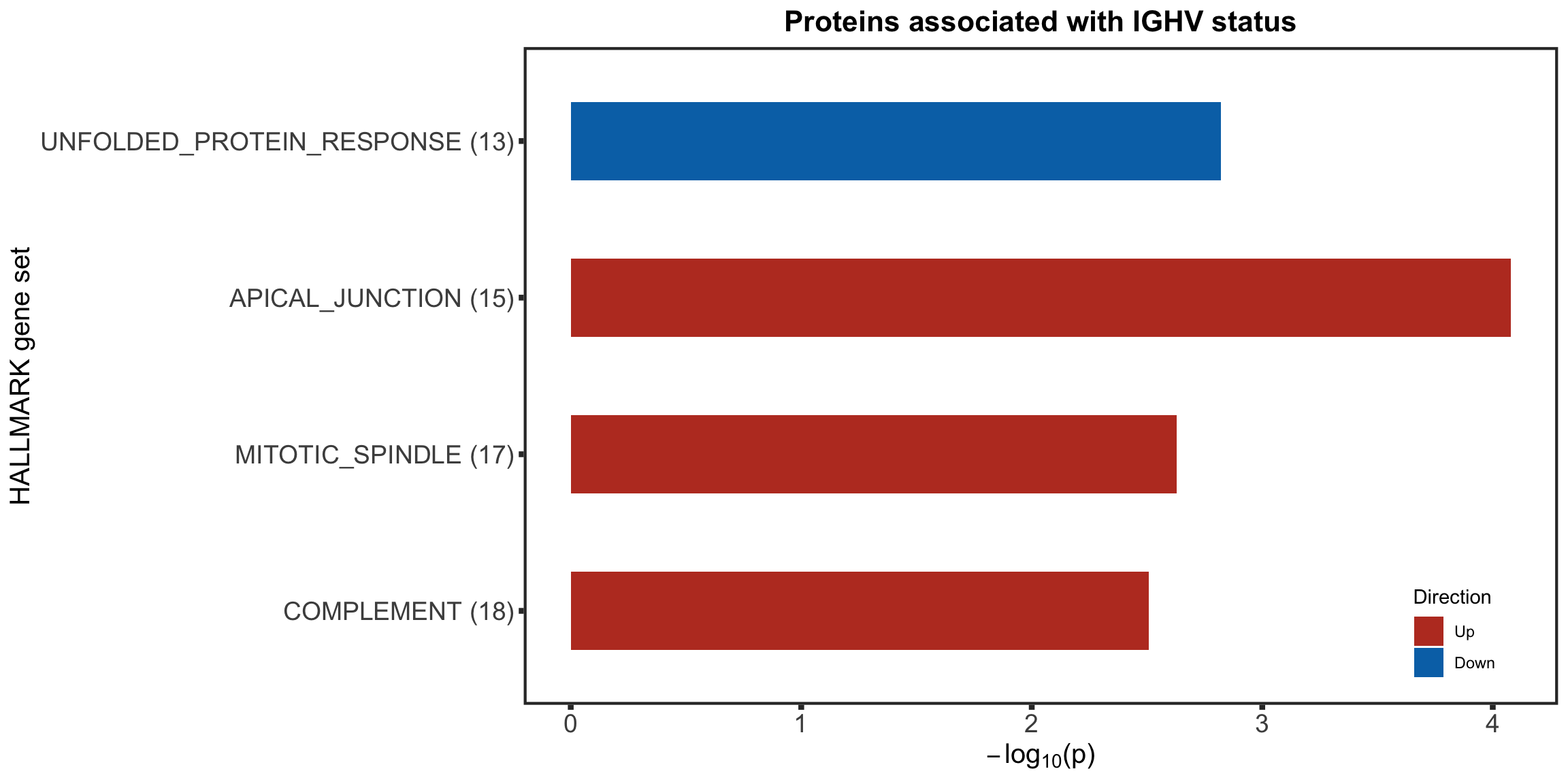
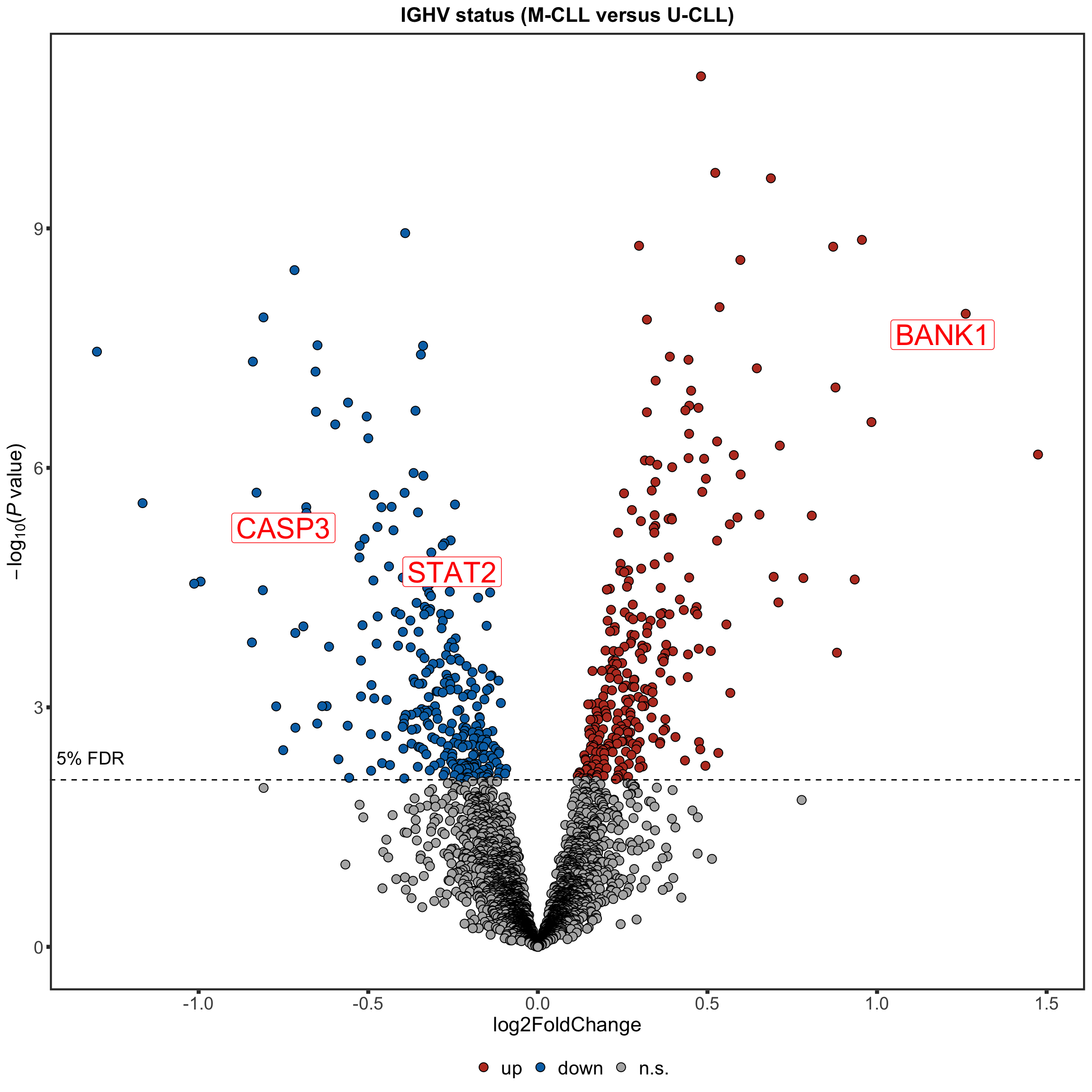
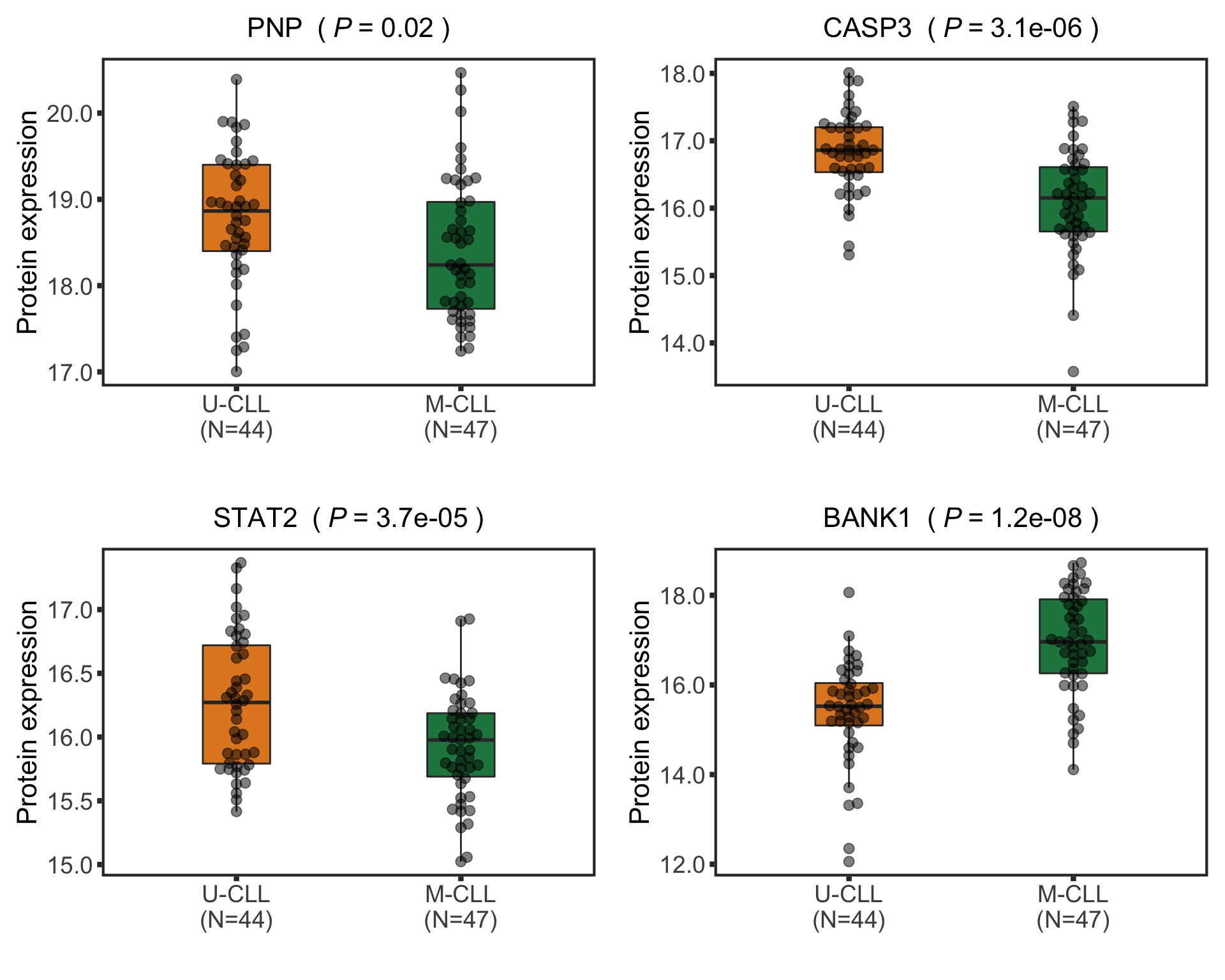
Protein abundance changes related to IGHV
fdrCut <- 0.05
protRes <- resList %>% filter(Gene == "IGHV.status") %>%
    dplyr::rename(uniprotID = id,
                  pvalue = P.Value, padj = adj.P.Val,
                  chrom = Chr) %>%
    mutate(geneID = rowData(protCLL[uniprotID,])$ensembl_gene_id) %>%
    select(name, uniprotID, geneID, chrom, logFC, pvalue, padj) %>%
    arrange(pvalue) %>% as_tibble()
Combine
allRes <- left_join(protRes, rnaRes, by = "geneID")
Construct protein-protein interaction network by “cause” proteins and “effect” proteins
fdrCut <- 0.05
resTab <- select(allRes, name, uniprotID, chrom, padj, padj.rna, logFC, log2FC.rna) %>%
  mutate(sigProt = padj <= fdrCut,
         sigRna = padj.rna <=fdrCut,
         upProt = logFC > 0,
         upRna = log2FC.rna >0)
comTab <- int_pairs %>% select(ProtA, ProtB, database) %>%
  left_join(resTab, by = c(ProtA = "uniprotID")) %>%
  left_join(resTab, by = c(ProtB = "uniprotID"))

comTab.filter <- comTab %>%
  filter(sigProt.x, sigProt.y, logFC.x*logFC.y >0) %>%
  mutate(direct = ifelse(logFC.x >0, "stabilizing", "destabilizing")) %>%
  mutate(source = case_when(
    sigProt.x & sigRna.x & sigProt.y & !sigRna.y ~ name.x,
    sigProt.y & sigRna.y & sigProt.x & !sigRna.x ~ name.y)) %>%
  filter(!is.na(source)) %>%
  mutate(target = ifelse(name.x == source, name.y, name.x)) %>%
  select(source, target, direct)
#get node list
allNodes <- union(comTab.filter$source, comTab.filter$target)

nodeList <- data.frame(id = seq(length(allNodes))-1, name = allNodes, stringsAsFactors = FALSE) %>%
  mutate(causal = ifelse(name %in% comTab.filter$source, "cause", "effect"))

#get edge list
edgeList <- select(comTab.filter, source, target, direct) %>%
  dplyr::rename(Source = source, Target = target) %>%
  mutate(Source = nodeList[match(Source,nodeList$name),]$id,
         Target = nodeList[match(Target, nodeList$name),]$id) %>%
  data.frame(stringsAsFactors = FALSE)

net <- graph_from_data_frame(vertices = nodeList, d=edgeList, directed = FALSE)
tidyNet <- as_tbl_graph(net)
complexNet <- ggraph(tidyNet, layout = "igraph", algorithm = "nicely") +
  geom_edge_link(aes(linetype = direct),color = colList[3], width=1) +
  geom_node_point(aes(color =causal, shape = causal), size=6) +
  geom_node_text(aes(label = name), repel = TRUE, size=6) +
  scale_color_manual(values = c(cause = colList[1],effect = colList[2])) +
  scale_linetype_manual(values = c(stabilizing = "solid", destabilizing = "dashed"))+
  scale_edge_color_brewer(palette = "Set2") +
  theme_graph(base_family = "sans") + theme(legend.position = "none")
complexNet

 CD38 are not detected any more