Feature selection with LASSO
Preprocessing data
Proteomics data
expVar <- "STAT2"

protMat <- assays(protCLL)[["QRILC_combat"]]
rownames(protMat) <- rowData(protCLL)$hgnc_symbol

yVec <- protMat[expVar,]
protMat <- protMat[rownames(protMat) != expVar,]

## Pre-filter for significant associations
designMat <- model.matrix(~yVec)
fit <- lmFit(protMat, design = designMat)
fit2 <- eBayes(fit)
resTab <- topTable(fit2, number = Inf)
keepProt <- filter(resTab, adj.P.Val < 0.1)$ID
protMat <- t(protMat[keepProt, ])
dim(protMat)
[1] 91 627
responseList <- list()
responseList[["STAT2"]] <- yVec

colnames(protMat) <- paste0(colnames(protMat),"_protein")
RNAseq
#subset
ddsSub <- dds[,dds$PatID %in% colnames(protCLL)]

#only keep protein coding genes with symbol
ddsSub <- ddsSub[rowData(ddsSub)$biotype %in% "protein_coding" & !rowData(ddsSub)$symbol %in% c("",NA),]

#remove lowly expressed genes
ddsSub <- ddsSub[rowSums(counts(ddsSub, normalized = TRUE)) > 100,]

#voom transformation
exprMat <- limma::voom(counts(ddsSub), lib.size = ddsSub$sizeFactor)$E
ddsSub.voom <- ddsSub
assay(ddsSub.voom) <- exprMat

rnaMat <- exprMat
rownames(rnaMat) <- rowData(ddsSub.voom)$symbol
# Prefiltering
overSampe <- intersect(names(yVec), colnames(rnaMat))
designMat <- model.matrix(~ yVec[overSampe])
fit <- lmFit(rnaMat[,overSampe], design = designMat)
fit2 <- eBayes(fit)
resTab <- topTable(fit2, number = Inf) %>% data.frame() %>% rownames_to_column("ID")
keepRna <- filter(resTab, adj.P.Val < 0.05)$ID
rnaMat <- t(rnaMat[keepRna, ])
dim(rnaMat)
[1] 82 704
colnames(rnaMat) <- paste0(colnames(rnaMat),"_rna")
Genomic data
ighvMap <- c(M = 1, U=0)
methMap <- c(LP= 0, IP=0.5, HP=1 )

#genetics
genData <- filter(patMeta, Patient.ID %in% colnames(protCLL)) %>%
  select(-HIPO.ID, -project, -date.of.diagnosis, -treatment, -date.of.first.treatment,
         -gender, -diagnosis, -Methylation_Cluster) %>%
  dplyr::rename(IGHV = IGHV.status) %>%
  mutate_at(vars(-Patient.ID), as.character) %>%
  mutate(IGHV = ighvMap[IGHV]) %>%
  mutate_at(vars(-Patient.ID), as.numeric) %>%
  data.frame() %>% column_to_rownames("Patient.ID")

#remove gene with higher than 40% missing values
genData <- genData[,colSums(is.na(genData))/nrow(genData) <= 0.4]

#remove genes with less than 5 mutated cases
genData <- genData[,colSums(genData, na.rm = TRUE) >= 5]

#fill the missing value with majority
genData <- apply(genData, 2, function(x) {
  xVec <- x
  avgVal <- mean(x,na.rm= TRUE)
  if (avgVal >= 0.5) {
    xVec[is.na(xVec)] <- 1
  } else xVec[is.na(xVec)] <- 0
  xVec
})
Drug responses
#choose the first sample
viabMat <- arrange(pheno1000_main, screenDate) %>%
  filter(diagnosis == "CLL", patientID %in% colnames(protCLL)) %>%
  distinct(patientID, Drug, concIndex, .keep_all = TRUE) %>%
  filter(! Drug %in% c("DMSO","PBS")) %>%
  mutate(id = paste0(Drug,"_",concIndex)) %>%
  select(patientID, id, normVal.adj.sigm) %>%
  spread(key = patientID, value = normVal.adj.sigm) %>%
  data.frame() %>% column_to_rownames("id") %>%
  as.matrix() %>% t()
Feature selection with LASSO penalty
#Functions for running glm
runGlm <- function(X, y, method = "ridge", repeats=20, folds = 3, lambda = "lambda.1se") {
  modelList <- list()
  lambdaList <- c()
  varExplain <- c()
  coefMat <- matrix(NA, ncol(X), repeats)
  rownames(coefMat) <- colnames(X)

  if (method == "lasso"){
    alpha = 1
  } else if (method == "ridge") {
    alpha = 0
  }

  for (i in seq(repeats)) {
    if (ncol(X) > 2) {
      res <- cv.glmnet(X,y, type.measure = "mse", family="gaussian",
                       nfolds = folds, alpha = alpha, standardize = FALSE)
      lambdaList <- c(lambdaList, res[[lambda]])
      modelList[[i]] <- res

      coefModel <- coef(res, s = lambda)[-1] #remove intercept row
      coefMat[,i] <- coefModel

      #calculate variance explained
      y.pred <- predict(res, s = lambda, newx = X)
      varExp <- cor(as.vector(y),as.vector(y.pred))^2
      varExplain[i] <- ifelse(is.na(varExp), 0, varExp)

    } else {
      fitlm<-lm(y~., data.frame(X))
      varExp <- summary(fitlm)$r.squared
      varExplain <- c(varExplain, varExp)

    }

  }
  list(modelList = modelList, lambdaList = lambdaList, varExplain = varExplain, coefMat = coefMat)
}
#function for scaling predictors
dataScale <- function(x, censor = NULL, robust = FALSE) {
        #function to scale different variables
        if (length(unique(na.omit(x))) <=3){
          #a binary variable, change to -0.5 and 0.5 for 1 and 2
          x - 0.5
        } else {
          if (robust) {
          #continuous variable, centered by median and divied by 2*mad
          mScore <- (x-median(x,na.rm=TRUE))/mad(x,na.rm=TRUE)
            if (!is.null(censor)) {
              mScore[mScore > censor] <- censor
              mScore[mScore < -censor] <- -censor
            }
          mScore/2
          } else {
            mScore <- (x-mean(x,na.rm=TRUE))/(sd(x,na.rm=TRUE))
              if (!is.null(censor)) {
                mScore[mScore > censor] <- censor
                mScore[mScore < -censor] <- -censor
              }
          mScore/2
          }
        }
      }
#function to generate response vector and explainatory variable for each seahorse measurement
generateData <- function(responseList, inclSet,  onlyCombine = FALSE, censor = NULL, robust = FALSE) {

    allResponse <- list()
    allExplain <- list()

    for (measure in names(responseList)) {
      y <- responseList[[measure]]
      y <- y[!is.na(y)]

      #get overlapped samples for each dataset
      overSample <- names(y)

      for (eachSet in inclSet) {
        overSample <- intersect(overSample,rownames(eachSet))
      }

      y <- dataScale(y[overSample], censor = censor, robust = robust)

      expTab <- list()

      if ("Gene" %in% names(inclSet)) {
        geneTab <- inclSet$Gene[overSample,]
        #at least 3 mutated sample
        geneTab <- geneTab[, colSums(geneTab) >= 3]
        vecName <- sprintf("genetic(%s)", ncol(geneTab))
        expTab[[vecName]] <- apply(geneTab,2,dataScale)
      }


      if ("RNA" %in% names(inclSet)){
        rnaMat <- inclSet$RNA[overSample, ]
        colnames(rnaMat) <- paste0("con.",colnames(rnaMat), sep = "")
        vecName <- sprintf("RNA(%s)", ncol(rnaMat))
        expTab[[vecName]] <- apply(rnaMat,2,dataScale, censor = censor, robust = robust)

      }

      if ("Protein" %in% names(inclSet)){
        protMat <- inclSet$Protein[overSample, ]
        colnames(protMat) <- paste0("con.",colnames(protMat), sep = "")
        vecName <- sprintf("Protein(%s)", ncol(protMat))
        expTab[[vecName]] <- apply(protMat,2,dataScale, censor = censor, robust = robust)

      }

      if ("Drug" %in% names(inclSet)){
        drugMat <- inclSet$Drug[overSample, ]
        colnames(drugMat) <- paste0("con.",colnames(drugMat), sep = "")
        vecName <- sprintf("Drug(%s)", ncol(drugMat))
        expTab[[vecName]] <- apply(drugMat,2,dataScale, censor = censor, robust = robust)

      }

      comboTab <- c()
      for (eachSet in names(expTab)){
        comboTab <- cbind(comboTab, expTab[[eachSet]])
      }
      vecName <- sprintf("all(%s)", ncol(comboTab))
      expTab[[vecName]] <- comboTab

      allResponse[[measure]] <- y
      allExplain[[measure]] <- expTab
    }
  if (onlyCombine) {
    #only return combined results, for feature selection
    allExplain <- lapply(allExplain, function(x) x[length(x)])
  }

  return(list(allResponse=allResponse, allExplain=allExplain))

}
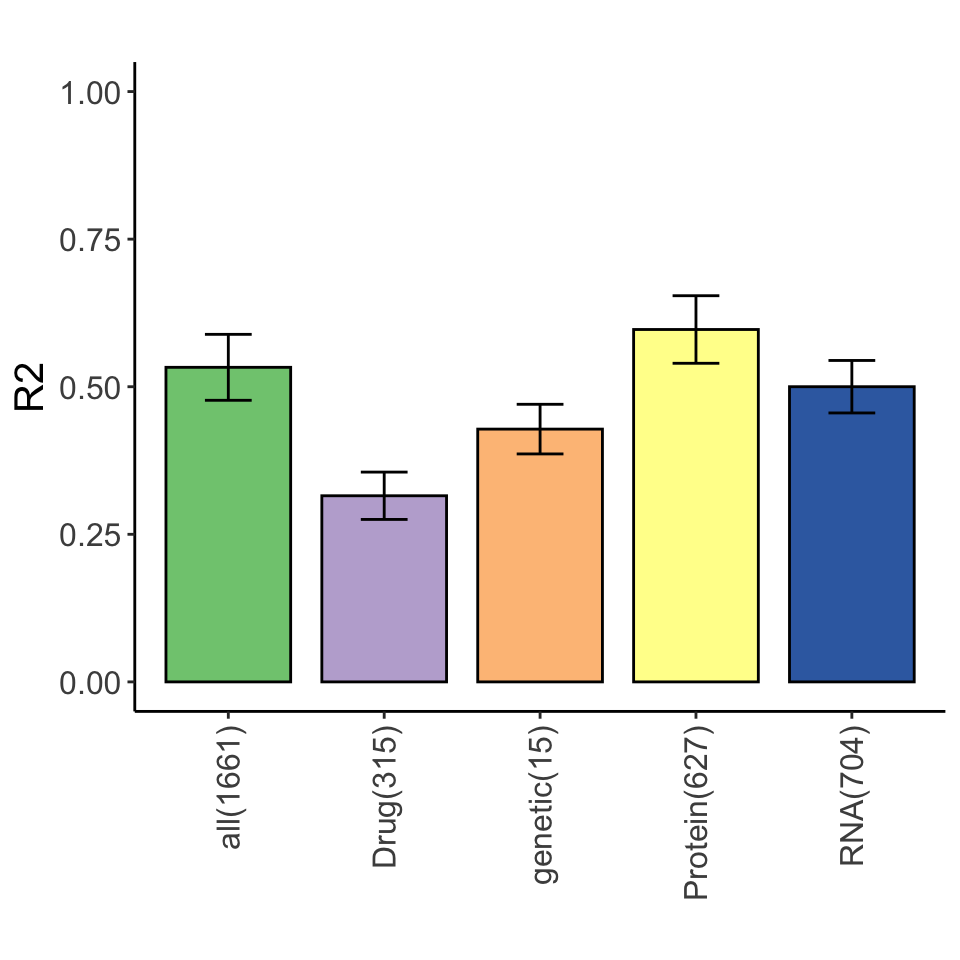
Clean and integrate multi-omics data
inclSet<-list(Gene=genData, RNA = rnaMat, Protein = protMat, Drug = viabMat)
cleanData <- generateData(responseList, inclSet, censor = 5)
#Function for multi-variate regression

runGlm <- function(X, y, method = "ridge", repeats=20, folds = 3) {
  modelList <- list()
  lambdaList <- c()
  varExplain <- c()
  coefMat <- matrix(NA, ncol(X), repeats)
  rownames(coefMat) <- colnames(X)

  if (method == "lasso"){
    alpha = 1
  } else if (method == "ridge") {
    alpha = 0
  }

  for (i in seq(repeats)) {
    if (ncol(X) > 2) {
      res <- cv.glmnet(X,y, type.measure = "mse", family="gaussian",
                       nfolds = folds, alpha = alpha, standardize = FALSE)
      lambdaList <- c(lambdaList, res$lambda.min)
      modelList[[i]] <- res

      coefModel <- coef(res, s = "lambda.min")[-1] #remove intercept row
      coefMat[,i] <- coefModel

      #calculate variance explained
      y.pred <- predict(res, s = "lambda.min", newx = X)

      varExp <- 1-min(res$cvm)/res$cvm[1]
      #varExp <- cor(as.vector(y),as.vector(y.pred))^2
      varExplain[i] <- ifelse(is.na(varExp), 0, varExp)

    } else {
      fitlm<-lm(y~., data.frame(X))
      varExp <- summary(fitlm)$r.squared
      varExplain <- c(varExplain, varExp)

    }

  }
  list(modelList = modelList, lambdaList = lambdaList, varExplain = varExplain, coefMat = coefMat)
}
set.seed(2020)
lassoResults <- list()
for (eachMeasure in names(cleanData$allResponse)) {
  dataResult <- list()
  for (eachDataset in names(cleanData$allExplain[[eachMeasure]])) {
    y <- cleanData$allResponse[[eachMeasure]]
    X <- cleanData$allExplain[[eachMeasure]][[eachDataset]]


    glmRes <- runGlm(X, y, method = "lasso", repeats = 50, folds = 3)
    dataResult[[eachDataset]] <- glmRes
  }
  lassoResults[[eachMeasure]] <- dataResult

}
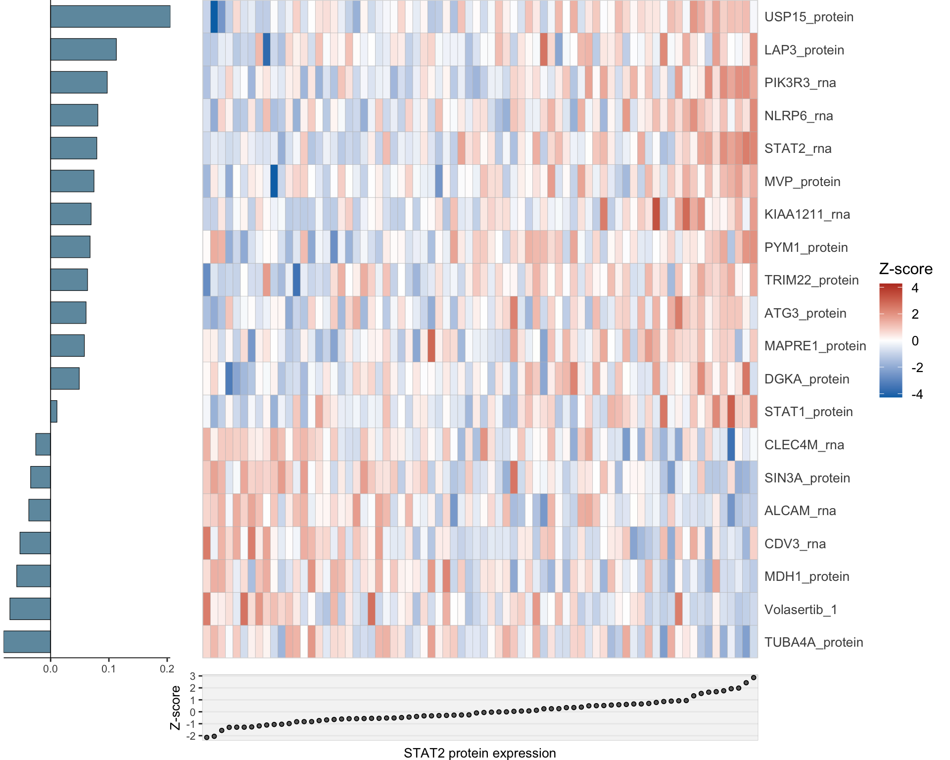
Variance explained for STAT2 expression by multi-omics datasets
Heatmap of selected features
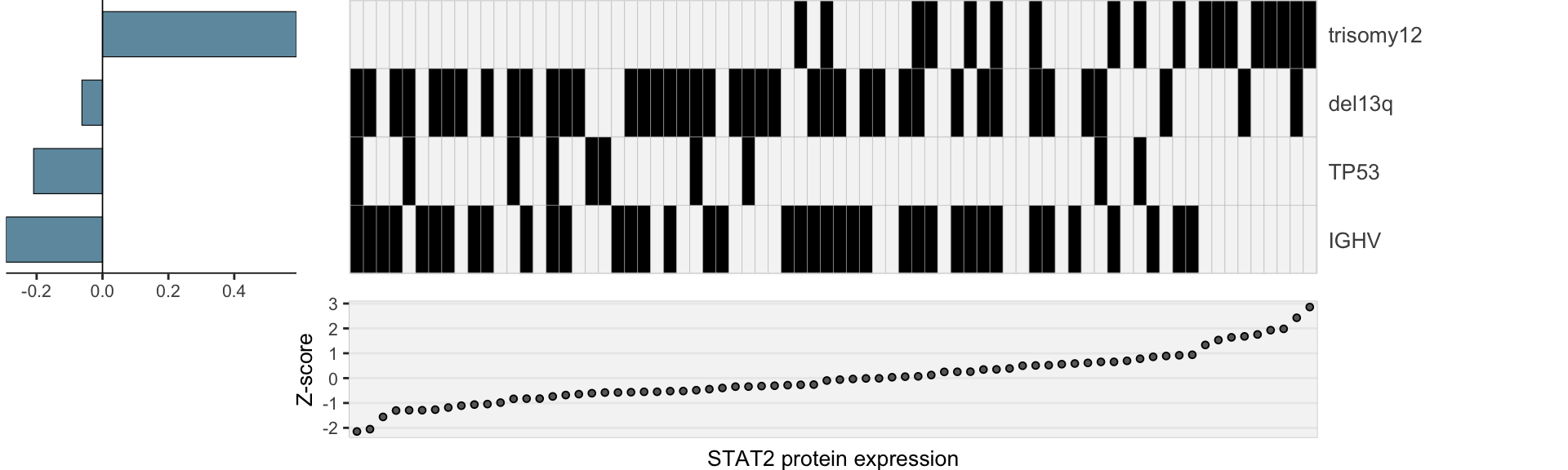
library(gtable)
lassoPlot <- function(lassoOut, cleanData, freqCut = 1, coefCut = 0.01, setNumber = "last", legend = TRUE, labSuffix = " protein expression", scaleFac =1) {
  plotList <- list()
  if (setNumber == "last") {
    setNumber <- length(lassoOut[[1]])
  } else {
    setNumber <- setNumber
  }
  for (seaName in names(lassoOut)) {
    #for the barplot on the left of the heatmap
    barValue <- rowMeans(lassoOut[[seaName]][[setNumber]]$coefMat)
    freqValue <- rowMeans(abs(sign(lassoOut[[seaName]][[setNumber]]$coefMat)))
    barValue <- barValue[abs(barValue) >= coefCut & freqValue >= freqCut] # a certain threshold
    barValue <- barValue[order(barValue)]
    if(length(barValue) == 0) {
      plotList[[seaName]] <- NA
      next
    }

    #for the heatmap and scatter plot below the heatmap
    allData <- cleanData$allExplain[[seaName]][[setNumber]]
    seaValue <- cleanData$allResponse[[seaName]]*2 #back to Z-score

    tabValue <- allData[, names(barValue),drop=FALSE]
    ord <- order(seaValue)
    seaValue <- seaValue[ord]
    tabValue <- tabValue[ord, ,drop=FALSE]
    sampleIDs <- rownames(tabValue)
    tabValue <- as.tibble(tabValue)

    #change scaled binary back to catagorical
    for (eachCol in colnames(tabValue)) {
      if (strsplit(eachCol, split = "[.]")[[1]][1] != "con") {
        tabValue[[eachCol]] <- as.integer(as.factor(tabValue[[eachCol]]))
      }
      else {
        tabValue[[eachCol]] <- tabValue[[eachCol]]*2 #back to Z-score
      }
    }

    tabValue$Sample <- sampleIDs
    #Mark different rows for different scaling in heatmap
    matValue <- gather(tabValue, key = "Var",value = "Value", -Sample)
    matValue$Type <- "mut"

    #For continuious value
    matValue$Type[grep("con.",matValue$Var)] <- "con"

    #for methylation_cluster
    matValue$Type[grep("ConsCluster",matValue$Var)] <- "meth"

    #change the scale of the value, let them do not overlap with each other
    matValue[matValue$Type == "mut",]$Value = matValue[matValue$Type == "mut",]$Value + 10
    matValue[matValue$Type == "meth",]$Value = matValue[matValue$Type == "meth",]$Value + 20


    #color scale for viability
    idx <- matValue$Type == "con"

    myCol <- colorRampPalette(c(colList[2],'white',colList[1]),
                   space = "Lab")
    if (sum(idx) != 0) {
      matValue[idx,]$Value = round(matValue[idx,]$Value,digits = 2)
      minViab <- min(matValue[idx,]$Value)
      maxViab <- max(matValue[idx,]$Value)
      limViab <- max(c(abs(minViab), abs(maxViab)))
      scaleSeq1 <- round(seq(-limViab, limViab,0.01), digits=2)
      color4viab <- setNames(myCol(length(scaleSeq1+1)), nm=scaleSeq1)
    } else {
      scaleSeq1 <- round(seq(0,1,0.01), digits=2)
      color4viab <- setNames(myCol(length(scaleSeq1+1)), nm=scaleSeq1)
    }


    #change continues measurement to discrete measurement
    matValue$Value <- factor(matValue$Value,levels = sort(unique(matValue$Value)))

    #change order of heatmap
    names(barValue) <-  gsub("con.", "", names(barValue))
    matValue$Var <- gsub("con.","",matValue$Var)
    matValue$Var <- factor(matValue$Var, levels = names(barValue))
    matValue$Sample <- factor(matValue$Sample, levels = names(seaValue))
    #plot the heatmap
    p1 <- ggplot(matValue, aes(x=Sample, y=Var)) + geom_tile(aes(fill=Value), color = "gray") +
      theme_bw() + scale_y_discrete(expand=c(0,0),position = "right") +
      theme(axis.text.y=element_text(hjust=0, size=10*scaleFac), axis.text.x=element_blank(),
            axis.title = element_blank(),
            axis.ticks=element_blank(), panel.border=element_rect(colour="gainsboro"),
            plot.title=element_blank(), panel.background=element_blank(),
            panel.grid.major=element_blank(), panel.grid.minor=element_blank(),
            plot.margin = margin(0,0,0,0)) +
      scale_fill_manual(name="Mutated",  values=c(color4viab, `11`="gray96", `12`='black', `21`='lightgreen',
                                                       `22`='green',`23` = 'green4'),guide=FALSE) #+ ggtitle(seaName)

    #Plot the bar plot on the left of the heatmap
    barDF = data.frame(barValue, nm=factor(names(barValue),levels=names(barValue)))

    p2 <- ggplot(data=barDF, aes(x=nm, y=barValue)) +
      geom_bar(stat="identity", fill=colList[6], colour="black", position = "identity", width=.66, size=0.2) +
      theme_bw() + geom_hline(yintercept=0, size=0.3) + scale_x_discrete(expand=c(0,0.5)) +
      scale_y_continuous(expand=c(0,0)) + coord_flip() +
      theme(panel.grid.major=element_blank(), panel.background=element_blank(), axis.ticks.y = element_blank(),
            panel.grid.minor = element_blank(),
            axis.text.x =element_text(size=8*scaleFac),
            axis.text.y = element_blank(),
            axis.title = element_blank(),
            panel.border=element_blank(),plot.margin = margin(0,0,0,0))  + geom_vline(xintercept=c(0.5), color="black", size=0.6)

    #Plot the scatter plot under the heatmap

    # scatterplot below
    scatterDF = data.frame(X=factor(names(seaValue), levels=names(seaValue)), Y=seaValue)

    p3 <- ggplot(scatterDF, aes(x=X, y=Y)) + geom_point(shape=21, fill="dimgrey", colour="black", size=1.2) +
      xlab(paste0(seaName, labSuffix)) + ylab("Z-score") +
      theme_bw() +
      theme(panel.grid.minor=element_blank(), panel.grid.major.x=element_blank(),
            axis.title=element_text(size=10*scaleFac),
            axis.text.x=element_blank(), axis.ticks.x=element_blank(),
            axis.text.y=element_text(size=8*scaleFac),
            panel.border=element_rect(colour="dimgrey", size=0.1),
            panel.background=element_rect(fill="gray96"),plot.margin = margin(0,0,0,0))


    dummyGrob <- ggplot() + theme_void()

    #Scale bar for continuous variable
    if (legend) {
       Vgg = ggplot(data=data.frame(x=1, y=as.numeric(names(color4viab))), aes(x=x, y=y, color=y)) + geom_point() +
      scale_color_gradientn(name="Z-score", colours =color4viab) +
      theme(legend.title=element_text(size=12*scaleFac), legend.text=element_text(size=10*scaleFac))
    barLegend <- plot_grid(gtable_filter(ggplotGrob(Vgg), "guide-box"))
    #Assemble all the plots togehter
    } else {
     barLegend <- dummyGrob
    }


    gt <- egg::ggarrange(p2,p1,barLegend,dummyGrob, p3, dummyGrob, ncol=3, nrow=2,
                         widths = c(0.6,2,0.3), padding = unit(0,"line"), clip = "off",
                         heights = c(length(unique(matValue$Var))/2,1),draw = FALSE)
    plotList[[seaName]] <- gt
  }
  return(plotList)
}
Genetics only
heatMaps <- lassoPlot(lassoResults, cleanData, freqCut = 1,setNumber = 1, legend = FALSE, scaleFac = 1)
heatMaps <- heatMaps[!is.na(heatMaps)]
geneLasso <- plot_grid(plotlist=heatMaps, ncol=1)
geneLasso
Combined
heatMaps <- lassoPlot(lassoResults, cleanData, freqCut = 1,setNumber = 5, legend = TRUE, scaleFac = 1)
heatMaps <- heatMaps[!is.na(heatMaps)]
comLasso <- plot_grid(plotlist=heatMaps, ncol=1)
comLasso
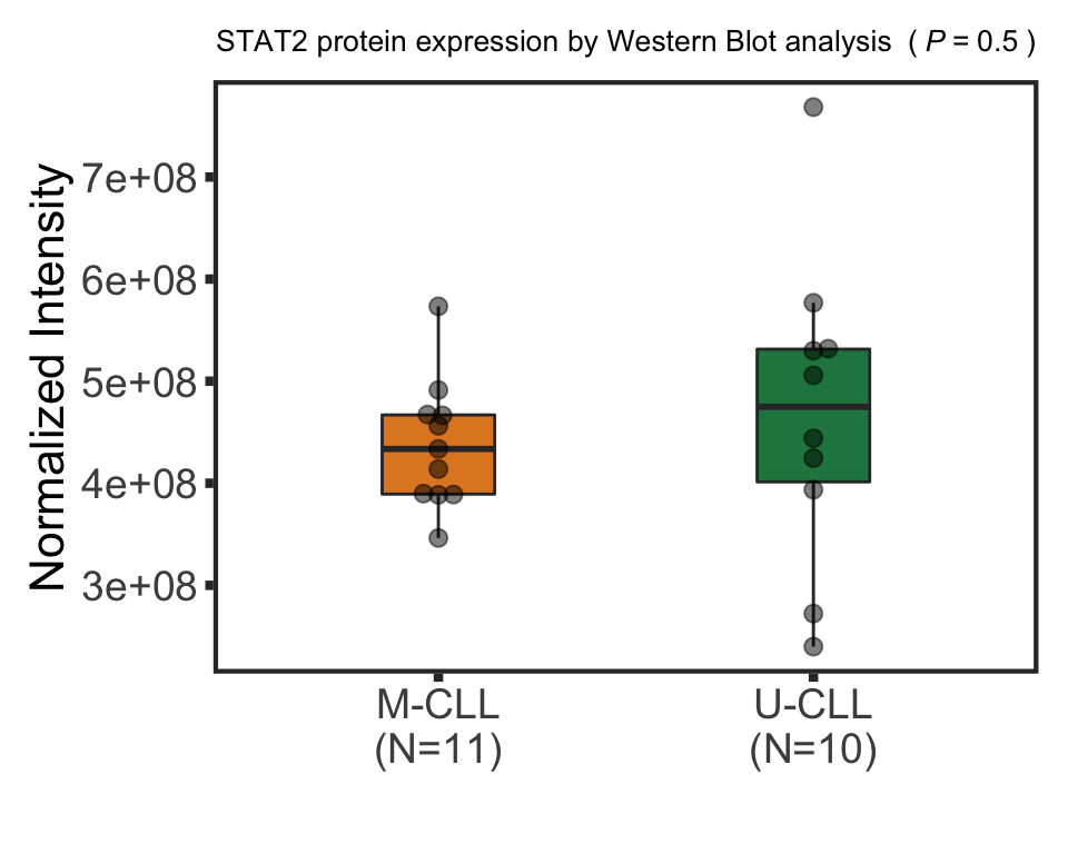
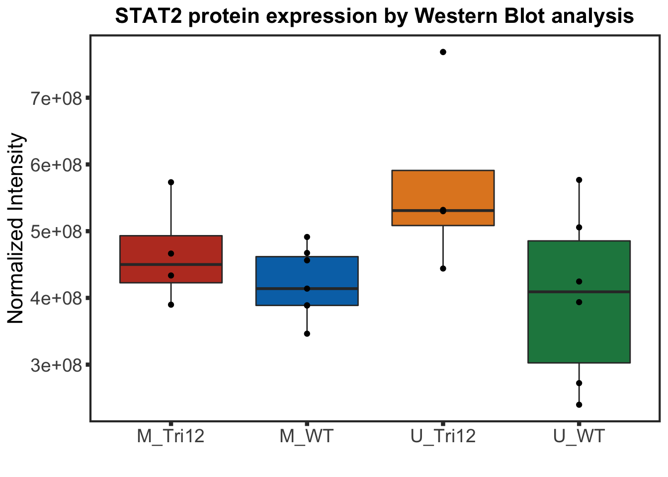
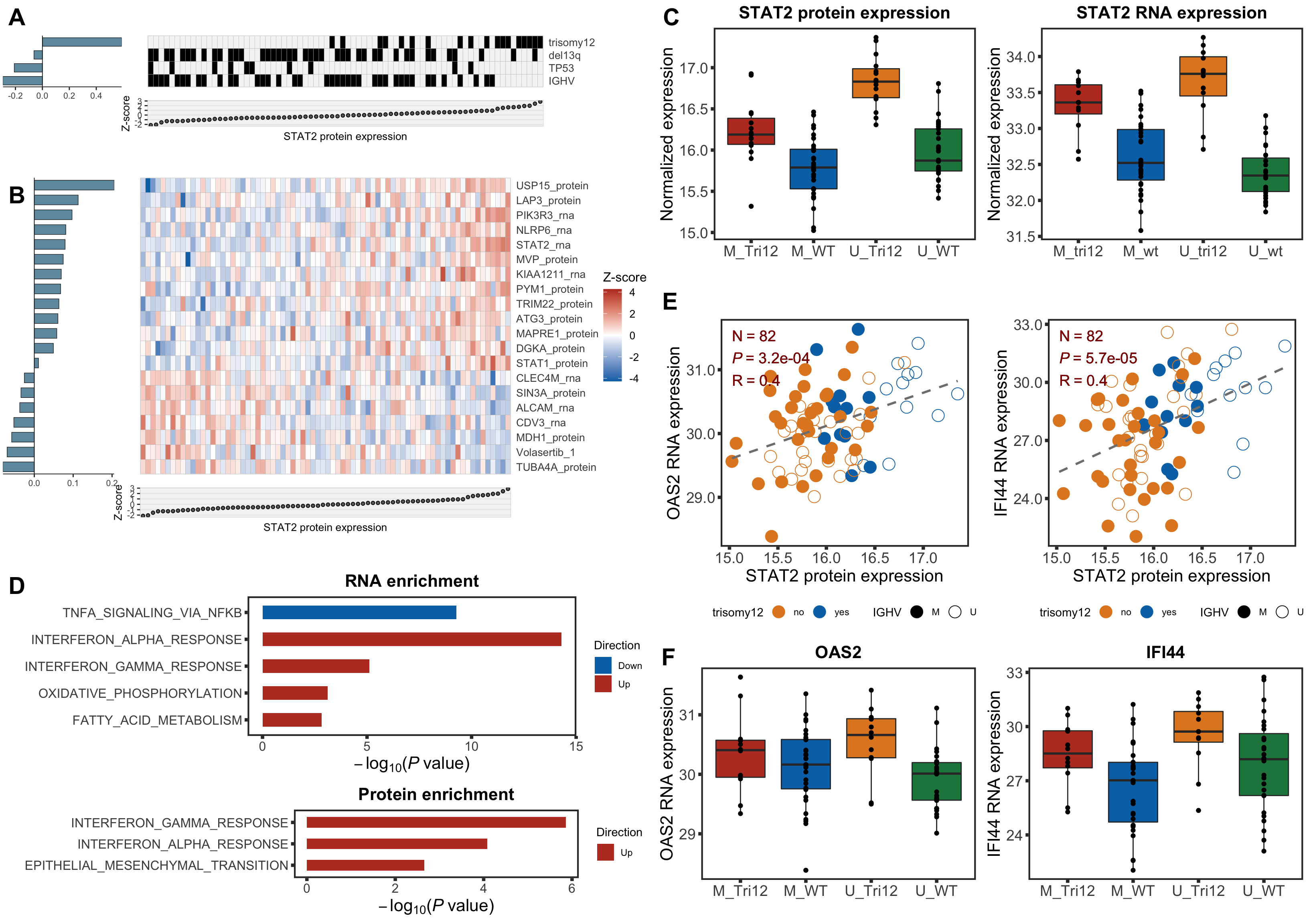
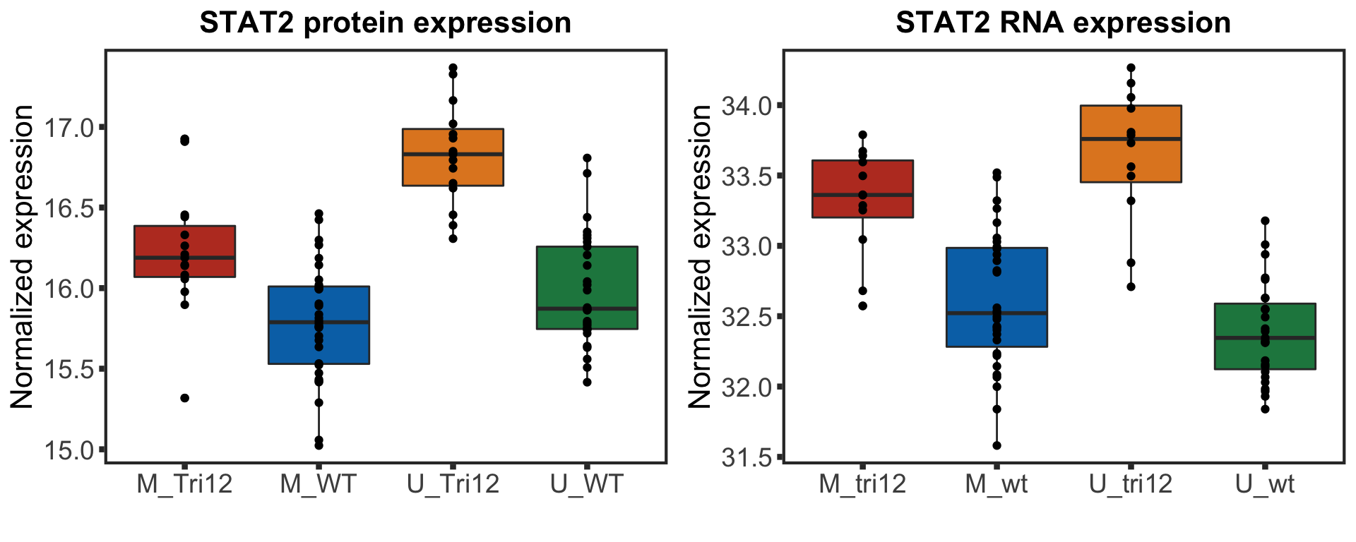
STAT2 protein expression stratified by IGHV and trisomy12
plotTab <- tibble(patID = colnames(protCLL),
                  STAT2 = assays(protCLL)[["count_combat"]][rowData(protCLL)$hgnc_symbol == "STAT2",],
                  trisomy12 = protCLL$trisomy12,
                  IGHV=protCLL$IGHV.status) %>%
  filter(!is.na(IGHV), !is.na(trisomy12)) %>%
  mutate(trisomy12 = ifelse(trisomy12 == 0, "WT","Tri12")) %>%
  mutate(group = paste0(IGHV, "_", trisomy12))
stat2BoxProt <- ggplot(plotTab, aes(group, y=STAT2, fill = group)) + geom_boxplot() + geom_point() + theme_full +
  scale_fill_manual(values = colList) + theme(legend.position = "none") +
  xlab("") + ggtitle("STAT2 protein expression") +ylab("Normalized expression")

summary(lm(STAT2 ~ IGHV * trisomy12, plotTab))
Call:
lm(formula = STAT2 ~ IGHV * trisomy12, data = plotTab)

Residuals:
    Min      1Q  Median      3Q     Max
-0.9044 -0.2317 -0.0275  0.2222  0.8272

Coefficients:
                  Estimate Std. Error t value Pr(>|t|)
(Intercept)       16.22239    0.09137 177.538  < 2e-16 ***
IGHVU              0.60433    0.12922   4.677 1.06e-05 ***
trisomy12WT       -0.43065    0.11074  -3.889 0.000196 ***
IGHVU:trisomy12WT -0.41597    0.15789  -2.634 0.009974 **
---
Signif. codes:  0 '***' 0.001 '**' 0.01 '*' 0.05 '.' 0.1 ' ' 1

Residual standard error: 0.3539 on 87 degrees of freedom
Multiple R-squared:  0.5157,    Adjusted R-squared:  0.499
F-statistic: 30.87 on 3 and 87 DF,  p-value: 1.097e-13
STAT2 protein expression is strongly affected by IGHV and trisomy12 status, U-CLLs with trisomy12 shows significant up-regulation of STAT2
STAT2 RNA expression stratified by IGHV and trisomy12
Samples in the proteomic cohort
plotTab <- tibble(patID = colnames(ddsSub.voom),
                  STAT2 = assay(ddsSub.voom)[rowData(ddsSub.voom)$symbol == "STAT2",],
                  trisomy12 = patMeta[match(patID, patMeta$Patient.ID),]$trisomy12,
                  IGHV=patMeta[match(patID, patMeta$Patient.ID),]$IGHV.status) %>%
  mutate(trisomy12 = ifelse(trisomy12 == 0, "wt","tri12")) %>%
  mutate(group = paste0(IGHV, "_", trisomy12))

stat2BoxRNA <- ggplot(plotTab, aes(group, y=STAT2, fill = group)) + geom_boxplot() + geom_point() + theme_full +
  scale_fill_manual(values = colList) + theme(legend.position = "none") +
  xlab("") + ggtitle("STAT2 RNA expression") +ylab("Normalized expression")

summary(lm(STAT2 ~ IGHV * trisomy12, plotTab))
Call:
lm(formula = STAT2 ~ IGHV * trisomy12, data = plotTab)

Residuals:
     Min       1Q   Median       3Q      Max
-1.03193 -0.27905 -0.03574  0.32709  0.90706

Coefficients:
                  Estimate Std. Error t value Pr(>|t|)
(Intercept)        33.3132     0.1245 267.644  < 2e-16 ***
IGHVU               0.3326     0.1760   1.889  0.06257 .
trisomy12wt        -0.7005     0.1466  -4.778 8.16e-06 ***
IGHVU:trisomy12wt  -0.5541     0.2094  -2.646  0.00986 **
---
Signif. codes:  0 '***' 0.001 '**' 0.01 '*' 0.05 '.' 0.1 ' ' 1

Residual standard error: 0.4312 on 78 degrees of freedom
Multiple R-squared:  0.5446,    Adjusted R-squared:  0.5271
F-statistic: 31.09 on 3 and 78 DF,  p-value: 2.525e-13
stat2Box <- plot_grid(stat2BoxProt, stat2BoxRNA)
stat2Box
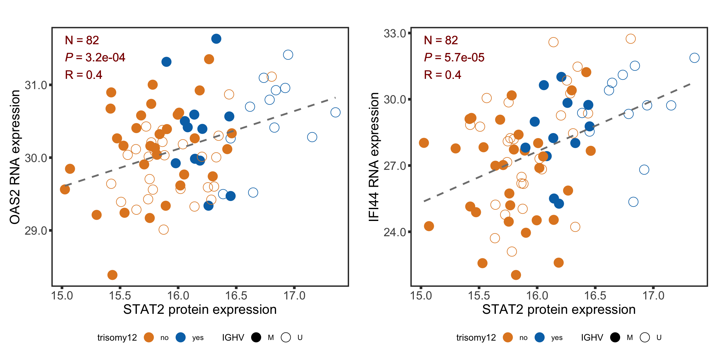
Pathway enrichment for RNA expressions correlated with STAT2 protein expression
expVar <- "STAT2"
protMat <- assays(protCLL)[["QRILC_combat"]]
rownames(protMat) <- rowData(protCLL)$hgnc_symbol
yVec <- protMat[expVar,]
Prepare data
#subset
ddsSub <- dds[,dds$PatID %in% names(yVec)]

#only keep protein coding genes with symbol
ddsSub <- ddsSub[rowData(ddsSub)$biotype %in% "protein_coding" & !rowData(ddsSub)$symbol %in% c("",NA),]

#remove lowly expressed genes
ddsSub <- ddsSub[rowSums(counts(ddsSub, normalized = TRUE)) > 100,]

#voom transformation
exprMat <- limma::voom(counts(ddsSub), lib.size = ddsSub$sizeFactor)$E
ddsSub.voom <- ddsSub
assay(ddsSub.voom) <- exprMat

rnaMat <- exprMat
rownames(rnaMat) <- rowData(ddsSub.voom)$symbol

overSampe <- intersect(names(yVec), colnames(rnaMat))

rnaMat <- rnaMat[,overSampe]
yVec <- yVec[overSampe]
Test
#buid design matirx
ighv <- patMeta[match(names(yVec),patMeta$Patient.ID),]$IGHV.status
tri12 <- patMeta[match(names(yVec),patMeta$Patient.ID),]$trisomy12

d0 <- model.matrix(~yVec)
d1 <- model.matrix(~ighv+tri12+yVec)
no blocking for IGHV or trisomy12
fit <- lmFit(rnaMat, design = d0)
fit2 <- eBayes(fit)
resTab.noBlock <- topTable(fit2, number = Inf, coef = "yVec") %>% data.frame() %>% rownames_to_column("name")
hist(resTab.noBlock$P.Value)

resTab.noBlock.sig <- filter(resTab.noBlock, adj.P.Val < 0.1)
resTab.noBlock %>% mutate_if(is.numeric, formatC, digits=2, format="e") %>% DT::datatable()
plotCorScatter <- function(plotTab, x_lab = "X", y_lab = "Y", title = "",
                           showR2 = FALSE, annoPos = "right",
                           dotCol = colList, textCol="darkred") {

  #prepare annotation values
  corRes <- cor.test(plotTab$x, plotTab$y)
  pval <- formatNum(corRes$p.value, digits = 1, format = "e")
  Rval <- formatNum(corRes$estimate, digits = 1, format = "e")
  R2val <- formatNum(corRes$estimate^2, digits = 1, format = "e")
  Nval <- nrow(plotTab)
  annoP <- bquote(italic("P")~"="~.(pval))

  if (showR2) {
    annoCoef <-  bquote(R^2~"="~.(R2val))
  } else {
    annoCoef <- bquote(R~"="~.(Rval))
  }
  annoN <- bquote(N~"="~.(Nval))

  corPlot <- ggplot(plotTab, aes(x = x, y = y)) + geom_point(aes(col = trisomy12, shape = IGHV), size=5) +
    scale_shape_manual(values = c(M = 19, U = 1)) +
    scale_color_manual(values = c(yes = colList[2], no = colList[3])) +
    geom_smooth(formula = y~x,method = "lm", se=FALSE, color = "grey50", linetype ="dashed" )

  if (annoPos == "right") {

    corPlot <- corPlot + annotate("text", x = max(plotTab$x), y = Inf, label = annoN,
                                  hjust=1, vjust =2, size = 5, parse = FALSE, col= textCol) +
      annotate("text", x = max(plotTab$x), y = Inf, label = annoP,
               hjust=1, vjust =4, size = 5, parse = FALSE, col= textCol) +
      annotate("text", x = max(plotTab$x), y = Inf, label = annoCoef,
               hjust=1, vjust =6, size = 5, parse = FALSE, col= textCol)

  } else if (annoPos== "left") {
    corPlot <- corPlot + annotate("text", x = min(plotTab$x), y = Inf, label = annoN,
                                  hjust=0, vjust =2, size = 5, parse = FALSE, col= textCol) +
      annotate("text", x = min(plotTab$x), y = Inf, label = annoP,
               hjust=0, vjust =4, size = 5, parse = FALSE, col= textCol) +
      annotate("text", x = min(plotTab$x), y = Inf, label = annoCoef,
               hjust=0, vjust =6, size = 5, parse = FALSE, col= textCol)
  }
  corPlot <- corPlot + ylab(y_lab) + xlab(x_lab) + ggtitle(title) +
    scale_y_continuous(labels = scales::number_format(accuracy = 0.1)) +
    scale_x_continuous(labels = scales::number_format(accuracy = 0.1)) +
    theme_full + theme(legend.position = "bottom", plot.margin = margin(12,12,12,12))
  corPlot
}
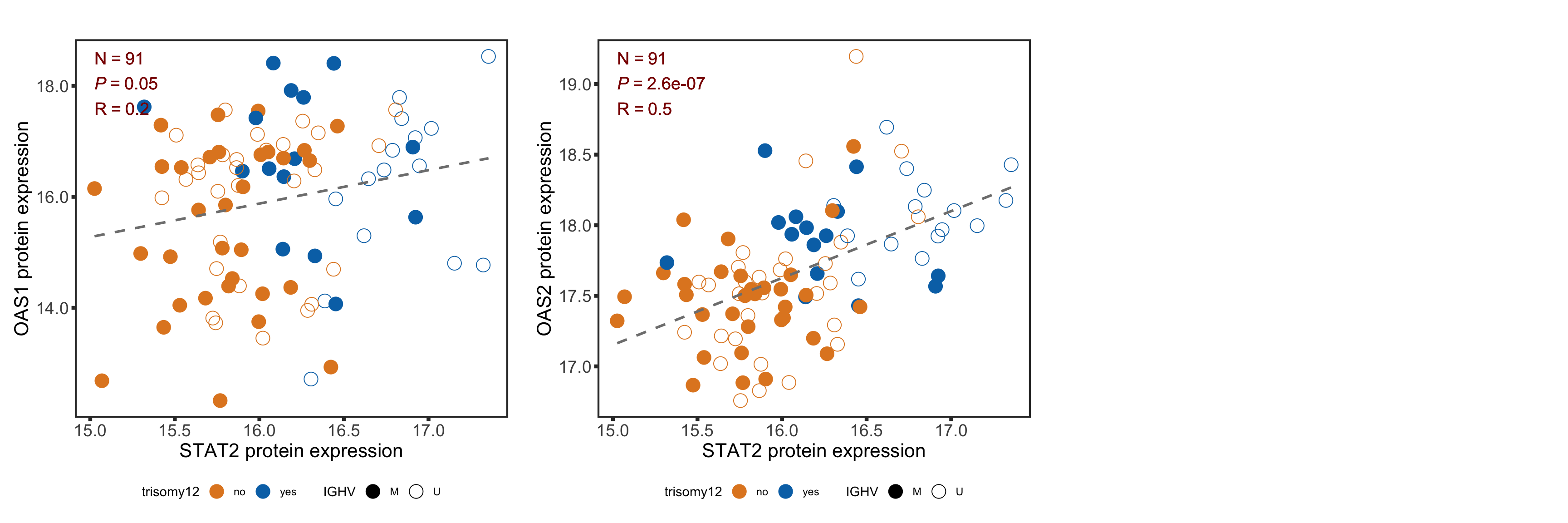
Correlation between selected genes and STAT2 protein expression
geneList <- c("OAS2", "IFI44")
rnaSTAT2cor <- lapply(geneList, function(n) {
  plotTab <- tibble(x = yVec, y = rnaMat[n,], IGHV = ighv, tri12 = tri12) %>%
    mutate(trisomy12 = ifelse(tri12==1,"yes","no"))
  plotCorScatter(plotTab, annoPos = "left", x_lab = "STAT2 protein expression", y_lab = sprintf("%s RNA expression", n))
})
names(rnaSTAT2cor) <- geneList
plotRNAcor <- plot_grid(plotlist = rnaSTAT2cor)
plotRNAcor
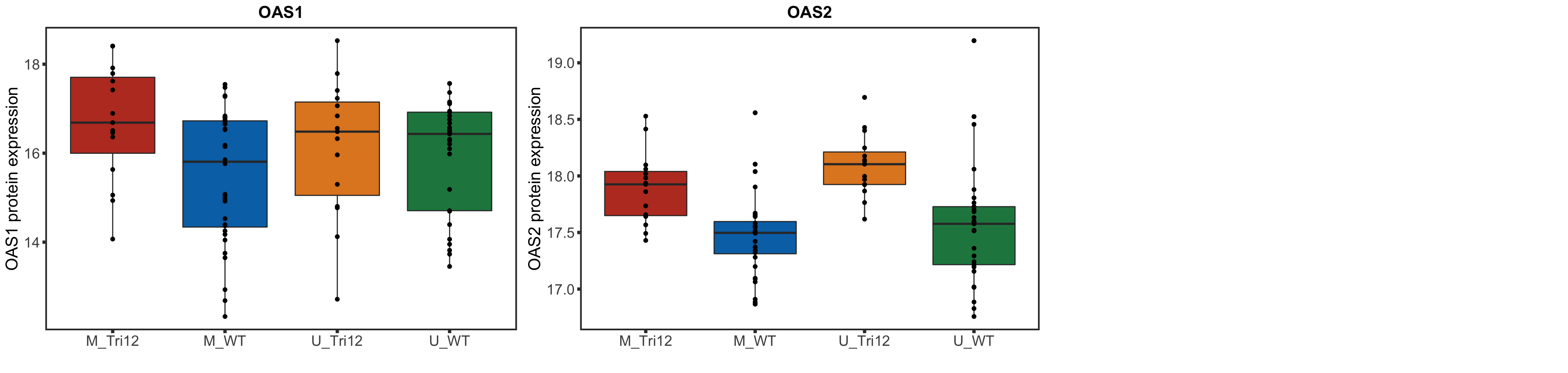
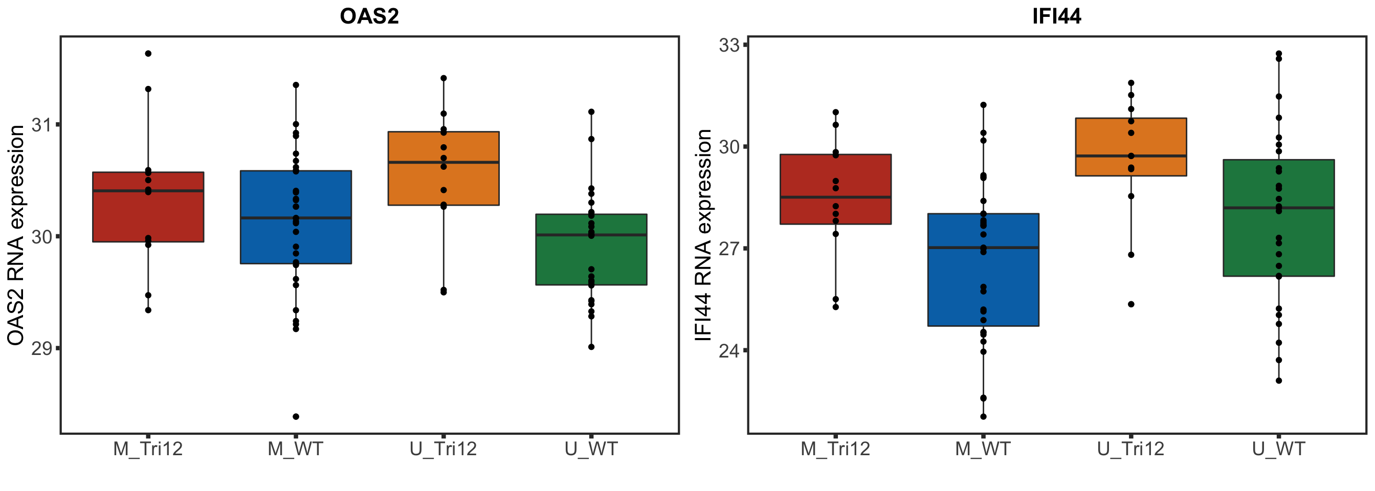
geneList <- c("OAS2", "IFI44")
rnaSTAT2corBox <- lapply(geneList, function(n) {
  plotTab <- tibble(expr = rnaMat[n,], IGHV = ighv, tri12 = tri12) %>%
  mutate(trisomy12 = ifelse(tri12==1,"Tri12","WT")) %>%
  mutate(group = paste0(IGHV, "_", trisomy12))

ggplot(plotTab, aes(group, y=expr, fill = group)) + geom_boxplot() + geom_point() + theme_full +
  scale_fill_manual(values = colList) + theme(legend.position = "none") +
  xlab("") + ylab(sprintf("%s RNA expression",n)) + ggtitle(n)
})
names(rnaSTAT2corBox) <- geneList
plotRNAbox <- plot_grid(plotlist = rnaSTAT2corBox)
plotRNAbox
gmts <- list(H = "../data/gmts/h.all.v6.2.symbols.gmt",
KEGG = "../data/gmts/c2.cp.kegg.v6.2.symbols.gmt")
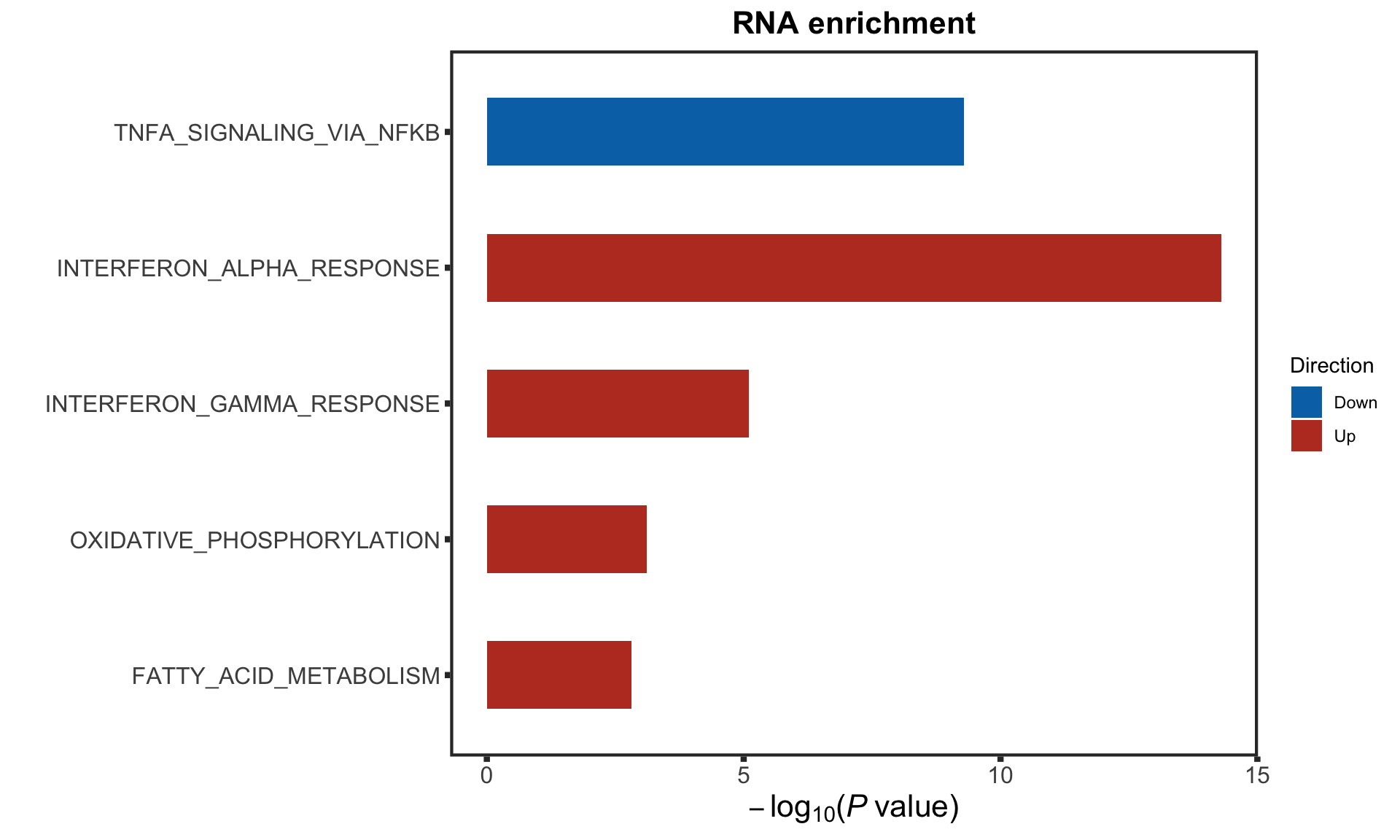
enRes <- runCamera(rnaMat, d0, gmts$H,
removePrefix = "HALLMARK_", pCut = 0.1, ifFDR = TRUE)
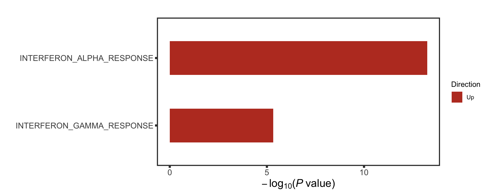
enRes$enrichPlot
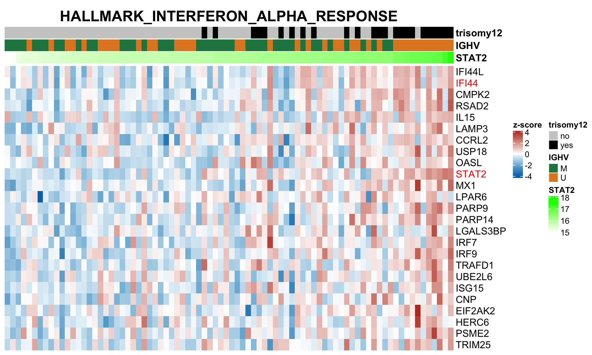
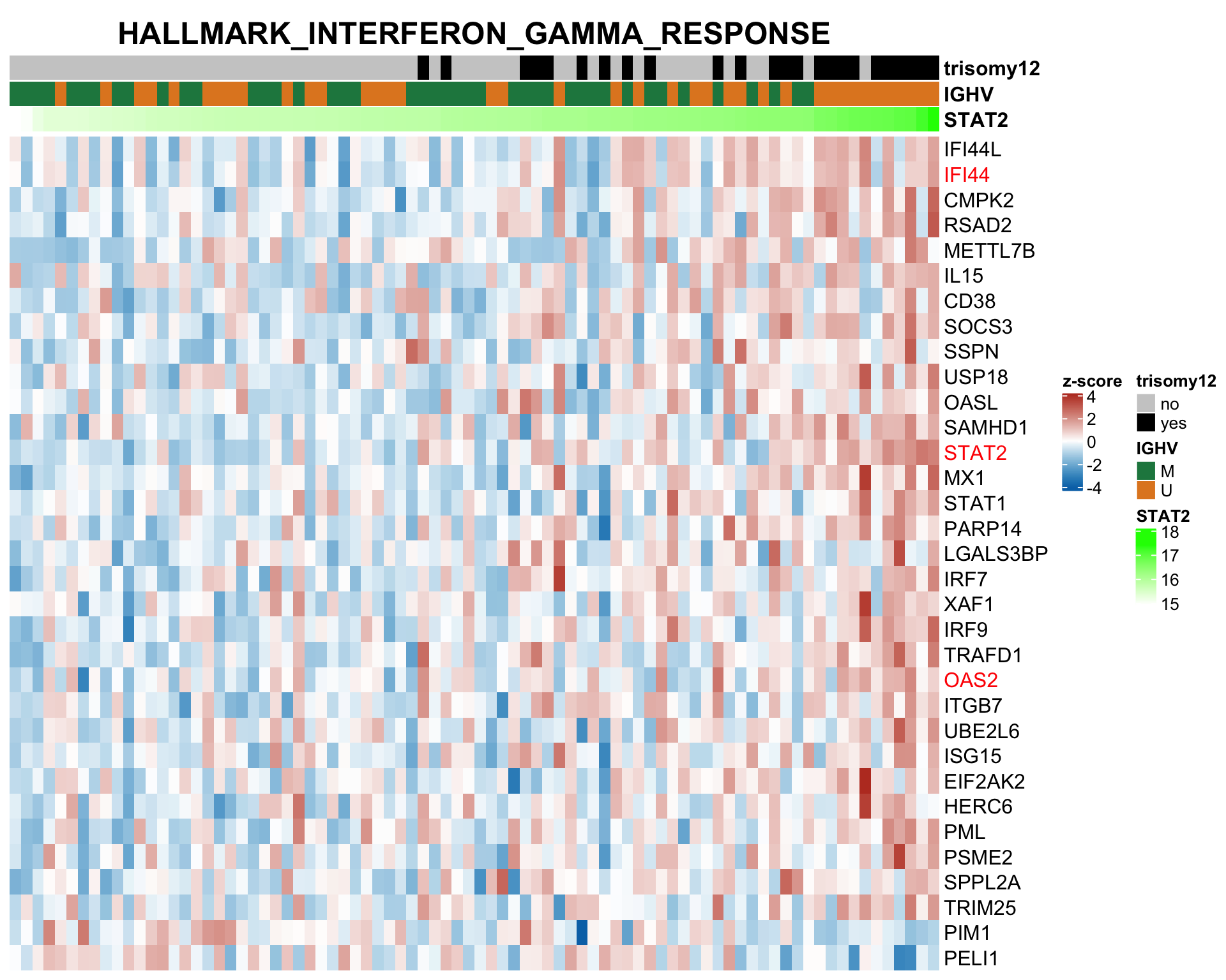
colAnno <- tibble(id = names(yVec), STAT2= yVec, IGHV = ighv, trisomy12 = tri12) %>%
mutate(trisomy12 = ifelse(trisomy12 ==1,"yes","no")) %>%
data.frame() %>% column_to_rownames("id")
annoCol <- list(trisomy12 = c(yes = "black",no = "grey80"),
IGHV = c(M = colList[4], U = colList[3]),
STAT2 = circlize::colorRamp2(c(min(colAnno$STAT2),max(colAnno$STAT2)),
c("white", "green")))
nameList <- c("STAT2","IFI44","OAS1","OAS2", "IFI30")
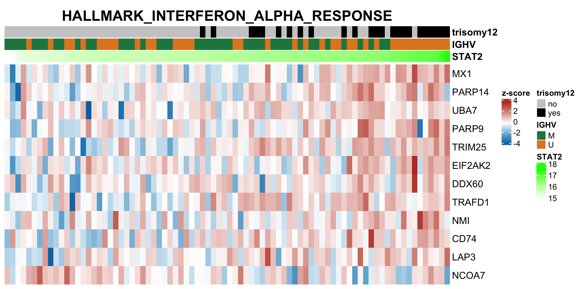
plotSetHeatmap(resTab.noBlock.sig, gmts$H, "HALLMARK_INTERFERON_ALPHA_RESPONSE", rnaMat, colAnno = colAnno, annoCol = annoCol, highLight = nameList)
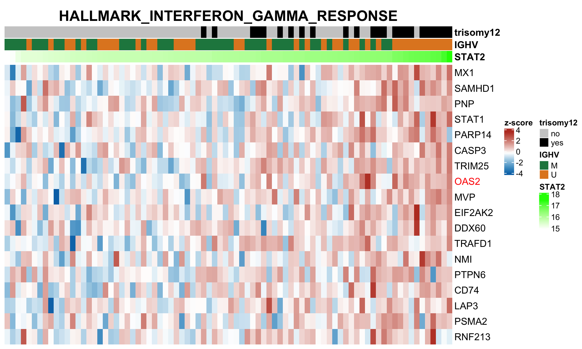
plotSetHeatmap(resTab.noBlock.sig, gmts$H, "HALLMARK_INTERFERON_GAMMA_RESPONSE", rnaMat, colAnno = colAnno, annoCol = annoCol,highLight = nameList)
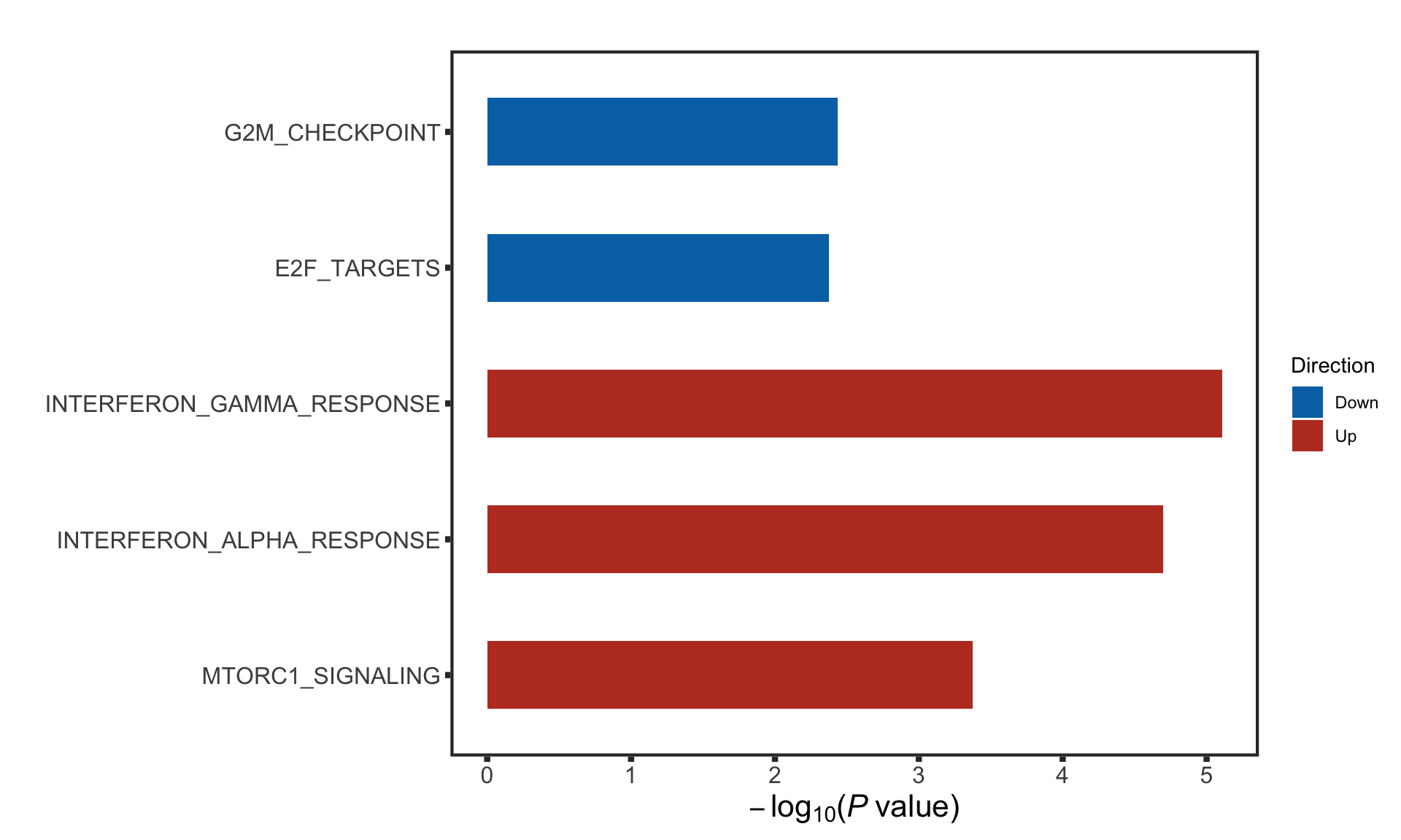
blocking for IGHV and trisomy12
fit <- lmFit(rnaMat, design = d1)
fit2 <- eBayes(fit)
resTab.block <- topTable(fit2, number = Inf, coef = "yVec") %>% data.frame() %>% rownames_to_column("name")
hist(resTab.block$P.Value)

resTab.block.sig <- filter(resTab.block, P.Value < 0.01)
enRes <- runCamera(rnaMat, d1, gmts$H, contrast = "yVec",
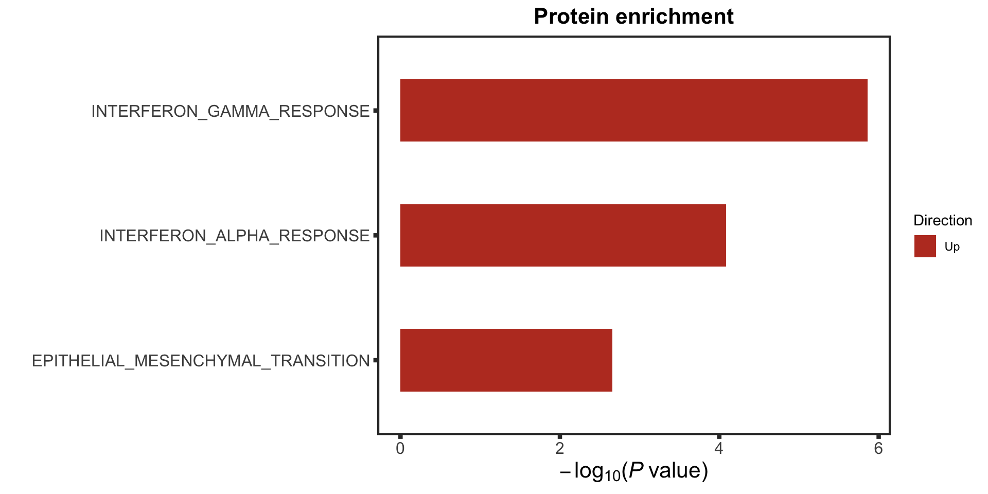
removePrefix = "HALLMARK_", pCut = 0.05, ifFDR = TRUE, plotTitle = "RNA enrichment")
rnaEnrich <- enRes$enrichPlot
rnaEnrich