Compare the results between LUMOS and timsTOF data
Junyan Lu
2020-02-27
Last updated: 2020-03-10
Checks: 7 0
Knit directory: Proteomics/analysis/
This reproducible R Markdown analysis was created with workflowr (version 1.6.0). The Checks tab describes the reproducibility checks that were applied when the results were created. The Past versions tab lists the development history.
Great! Since the R Markdown file has been committed to the Git repository, you know the exact version of the code that produced these results.
Great job! The global environment was empty. Objects defined in the global environment can affect the analysis in your R Markdown file in unknown ways. For reproduciblity it’s best to always run the code in an empty environment.
The command set.seed(20200227) was run prior to running the code in the R Markdown file. Setting a seed ensures that any results that rely on randomness, e.g. subsampling or permutations, are reproducible.
Great job! Recording the operating system, R version, and package versions is critical for reproducibility.
Nice! There were no cached chunks for this analysis, so you can be confident that you successfully produced the results during this run.
Great job! Using relative paths to the files within your workflowr project makes it easier to run your code on other machines.
Great! You are using Git for version control. Tracking code development and connecting the code version to the results is critical for reproducibility. The version displayed above was the version of the Git repository at the time these results were generated.
Note that you need to be careful to ensure that all relevant files for the analysis have been committed to Git prior to generating the results (you can use wflow_publish or wflow_git_commit). workflowr only checks the R Markdown file, but you know if there are other scripts or data files that it depends on. Below is the status of the Git repository when the results were generated:
Ignored files:
    Ignored:    .DS_Store
    Ignored:    .Rhistory
    Ignored:    .Rproj.user/
    Ignored:    analysis/.DS_Store
    Ignored:    analysis/.Rhistory
    Ignored:    analysis/compareProteomicsRNAseq_cache/
    Ignored:    analysis/correlateCLLPD_cache/
    Ignored:    analysis/correlateGenomic_cache/
    Ignored:    analysis/correlateGenomic_removePC_cache/
    Ignored:    analysis/correlateMIR_cache/
    Ignored:    analysis/correlateMethylationCluster_cache/
    Ignored:    analysis/predictOutcome_cache/
    Ignored:    data/.DS_Store
    Ignored:    output/.DS_Store

Untracked files:
    Untracked:  code/utils.R
    Untracked:  data/190909_CLL_prot_abund_med_norm.tsv
    Untracked:  data/190909_CLL_prot_abund_no_norm.tsv
    Untracked:  data/20190423_Proteom_submitted_samples_bereinigt.xlsx
    Untracked:  data/20191025_Proteom_submitted_samples_final.xlsx
    Untracked:  data/LUMOS/
    Untracked:  data/LUMOS_peptides/
    Untracked:  data/LUMOS_protAnnotation.csv
    Untracked:  data/SampleAnnotation_cleaned.xlsx
    Untracked:  data/facTab_IC50atLeast3New.RData
    Untracked:  data/gmts/
    Untracked:  data/mapEnsemble.txt
    Untracked:  data/mapSymbol.txt
    Untracked:  data/pyprophet_export_aligned.csv
    Untracked:  data/timsTOF_protAnnotation.csv
    Untracked:  output/LUMOS_processed.RData
    Untracked:  output/proteomic_LUMOS_20200227.RData
    Untracked:  output/proteomic_timsTOF_20200227.RData
    Untracked:  output/timsTOF_processed.RData
Note that any generated files, e.g. HTML, png, CSS, etc., are not included in this status report because it is ok for generated content to have uncommitted changes.
These are the previous versions of the R Markdown and HTML files. If you’ve configured a remote Git repository (see ?wflow_git_remote), click on the hyperlinks in the table below to view them.
| File | Version | Author | Date | Message |
|---|---|---|---|---|
| Rmd | b688c41 | Junyan Lu | 2020-02-27 | wflow_git_commit(all = TRUE) |
| html | b688c41 | Junyan Lu | 2020-02-27 | wflow_git_commit(all = TRUE) |
| html | 46534c2 | Junyan Lu | 2020-02-27 | Build site. |
| Rmd | 2b8852e | Junyan Lu | 2020-02-27 | wflow_publish(list.files(“./”, pattern = “Rmd”)) |
library(SummarizedExperiment)
library(jyluMisc)
library(tidyverse)
Load both datasets
load("../../var/proteomic_LUMOS_191119.RData")
protCLL.lumos.raw <- protCLL_raw
protCLL.lumos <- protCLL
load("../../var/proteomic_191105.RData")
protCLL.tof.raw <- protCLL_raw
protCLL.tof <- protCLL
Number of detected proteins
Overlap of all dectected proteins
library(Vennerable)
symbolList.all <- list(LUMOS = unique(rowData(protCLL.lumos.raw)$hgnc_symbol),
                   timsTOF = unique(rowData(protCLL.tof.raw)$hgnc_symbol))
Vpro <- Venn(symbolList.all)
plot(Vpro, doWeights = FALSE)
| Version | Author | Date |
|---|---|---|
| 46534c2 | Junyan Lu | 2020-02-27 |
Overlap of filtered proteins (less than 50% missing rate)
symbolList <- list(LUMOS = unique(rowData(protCLL.lumos)$hgnc_symbol),
                   timsTOF = unique(rowData(protCLL.tof)$hgnc_symbol))
Vpro <- Venn(symbolList)
plot(Vpro, doWeights = FALSE)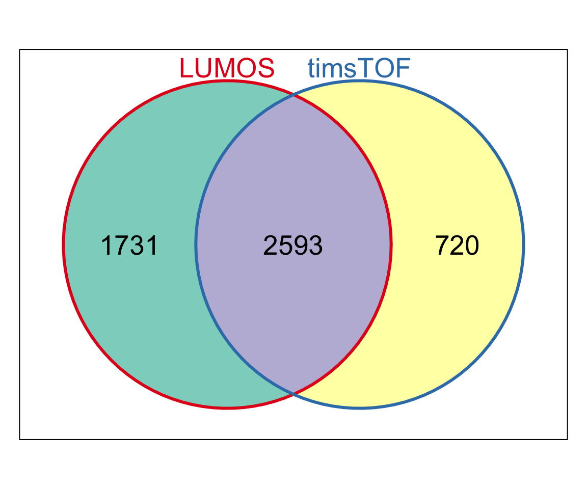
| Version | Author | Date |
|---|---|---|
| 46534c2 | Junyan Lu | 2020-02-27 |
Expression distribution of common and uniquely detected proteins
commonProtein <- intersect(symbolList.all$LUMOS, symbolList.all$timsTOF)
proteinGroup <- tibble(name = commonProtein, group = "both") %>%
  bind_rows(tibble(name = setdiff(symbolList.all$LUMOS, commonProtein), group = "LUMOS_only")) %>%
  bind_rows(tibble(name = setdiff(symbolList.all$timsTOF, commonProtein), group = "timsTOF_only"))

exprTab.lumos <- assay(protCLL.lumos.raw) %>% data.frame() %>%
  rownames_to_column("id") %>% mutate(name = rowData(protCLL.lumos.raw[id,])$hgnc_symbol) %>%
  gather(key = "patID", value = "expr", -id, -name) %>%
  mutate(group = proteinGroup[match(name, proteinGroup$name),]$group,
         dataset = "LUMOS")

exprTab.tof<- assay(protCLL.tof.raw) %>% data.frame() %>%
  rownames_to_column("id") %>% mutate(name = rowData(protCLL.tof.raw[id,])$hgnc_symbol) %>%
  gather(key = "patID", value = "expr", -id, -name) %>%
  mutate(group = proteinGroup[match(name, proteinGroup$name),]$group,
         dataset = "timsTOF")

exprTab <- bind_rows(exprTab.lumos, exprTab.tof)
ggplot(exprTab, aes(x = log10(expr), fill = group)) +
  geom_histogram(position = "identity", alpha = 0.5, bins=100, col = "grey50") +
  facet_wrap(~dataset) +
  xlab("log10(counts)")
Warning: Removed 45857 rows containing non-finite values (stat_bin).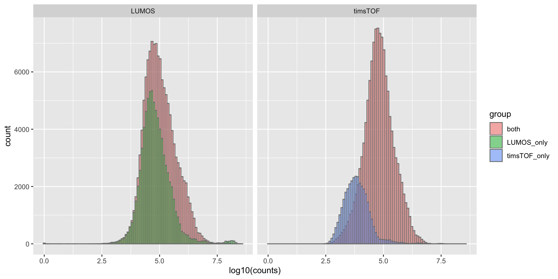
| Version | Author | Date |
|---|---|---|
| 46534c2 | Junyan Lu | 2020-02-27 |
Fraction of NA values
sumNAtab <- group_by(exprTab, group, dataset) %>%
  summarise(NAratio = sum(is.na(expr)/length(expr)))
ggplot(sumNAtab, aes(x=group, y=NAratio, fill = dataset)) + geom_bar(stat = "identity", position = "dodge") +
  ylab("Ratio of missing values") + xlab("")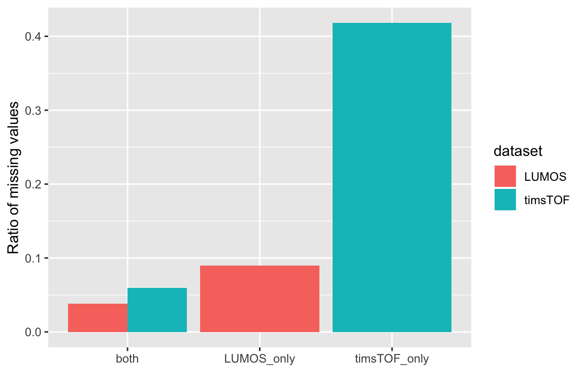
| Version | Author | Date |
|---|---|---|
| 46534c2 | Junyan Lu | 2020-02-27 |
Correlations of commonly detected proteins
Pearson correlation coefficient
sumProtein <- filter(exprTab, group == "both") %>%
  filter(!is.na(expr)) %>% group_by(id) %>%
  summarise(nLUMOS = sum(dataset == "LUMOS"),nTOF = sum(dataset=="timsTOF")) %>%
  filter(nLUMOS >= 10 & nTOF >=10 )

testRes <- filter(exprTab, group == "both", id %in% sumProtein$id) %>%
  mutate(expr = log(expr)) %>%
  spread(key = dataset, value = expr) %>%
  group_by(id) %>% nest() %>%
  mutate(m = map(data, ~cor.test(~LUMOS+timsTOF,.))) %>%
  mutate(res = map(m, broom::tidy)) %>%
  unnest(res)

ggplot(testRes, aes(x=estimate)) + geom_histogram(position = "identity", col = "grey50", alpha =0.3, bins =100) +
  geom_vline(xintercept = 0, col = "red", linetype = "dashed")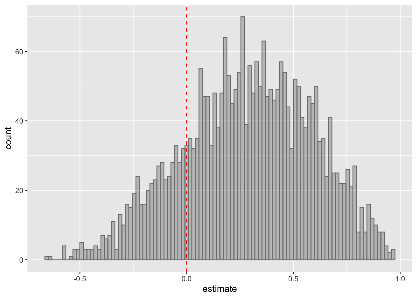
| Version | Author | Date |
|---|---|---|
| 46534c2 | Junyan Lu | 2020-02-27 |
Correlation between coefficient and NA fraction
naTab <- sumProtein <- filter(exprTab, group == "both") %>%
  select(id, patID, expr, dataset) %>%
  spread(key = dataset, value = expr) %>%
  group_by(id) %>%
  summarise(LUMOS.miss = sum(is.na(LUMOS)/length(LUMOS)),
           timsTOF.miss = sum(is.na(timsTOF)/length(LUMOS)))
plotTab <- left_join(testRes, naTab, by = "id") %>%
  select(id, estimate, LUMOS.miss, timsTOF.miss) %>%
  gather(key = "set", value = "missRatio", -id, -estimate)

ggplot(plotTab, aes(x=missRatio, y = estimate)) + geom_point() + geom_smooth(method="lm") +
  facet_wrap(~set)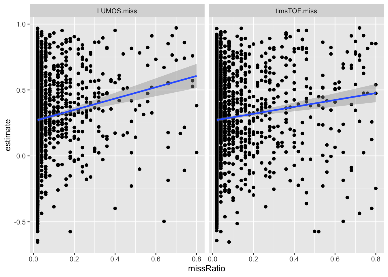
| Version | Author | Date |
|---|---|---|
| 46534c2 | Junyan Lu | 2020-02-27 |
Pathways that are enriched for more and less reproducible proteins
gmts = list(H= "../data/gmts/h.all.v6.2.symbols.gmt",
            C6 = "../data/gmts/c6.all.v6.2.symbols.gmt",
            KEGG = "../data/gmts/c2.cp.kegg.v6.2.symbols.gmt")
inputTab <- testRes %>% select(id, estimate) %>% ungroup() %>%
  mutate(name = rowData(protCLL.lumos.raw[id,])$hgnc_symbol) %>% filter(!is.na(name)) %>%
  arrange(estimate) %>% distinct(name, .keep_all = TRUE) %>% select(name, estimate) %>%
  data.frame() %>%
  column_to_rownames("name")
enRes <- list()
enRes[["HALLMARK"]] <- jyluMisc::runGSEA(inputTab, gmts$H, "page")
Loading required package: pianoenRes[["C6"]] <- jyluMisc::runGSEA(inputTab, gmts$C6, "page")
p <- jyluMisc::plotEnrichmentBar(enRes, pCut =0.05, ifFDR= TRUE)Coordinate system already present. Adding new coordinate system, which will replace the existing one.Coordinate system already present. Adding new coordinate system, which will replace the existing one.plot(p)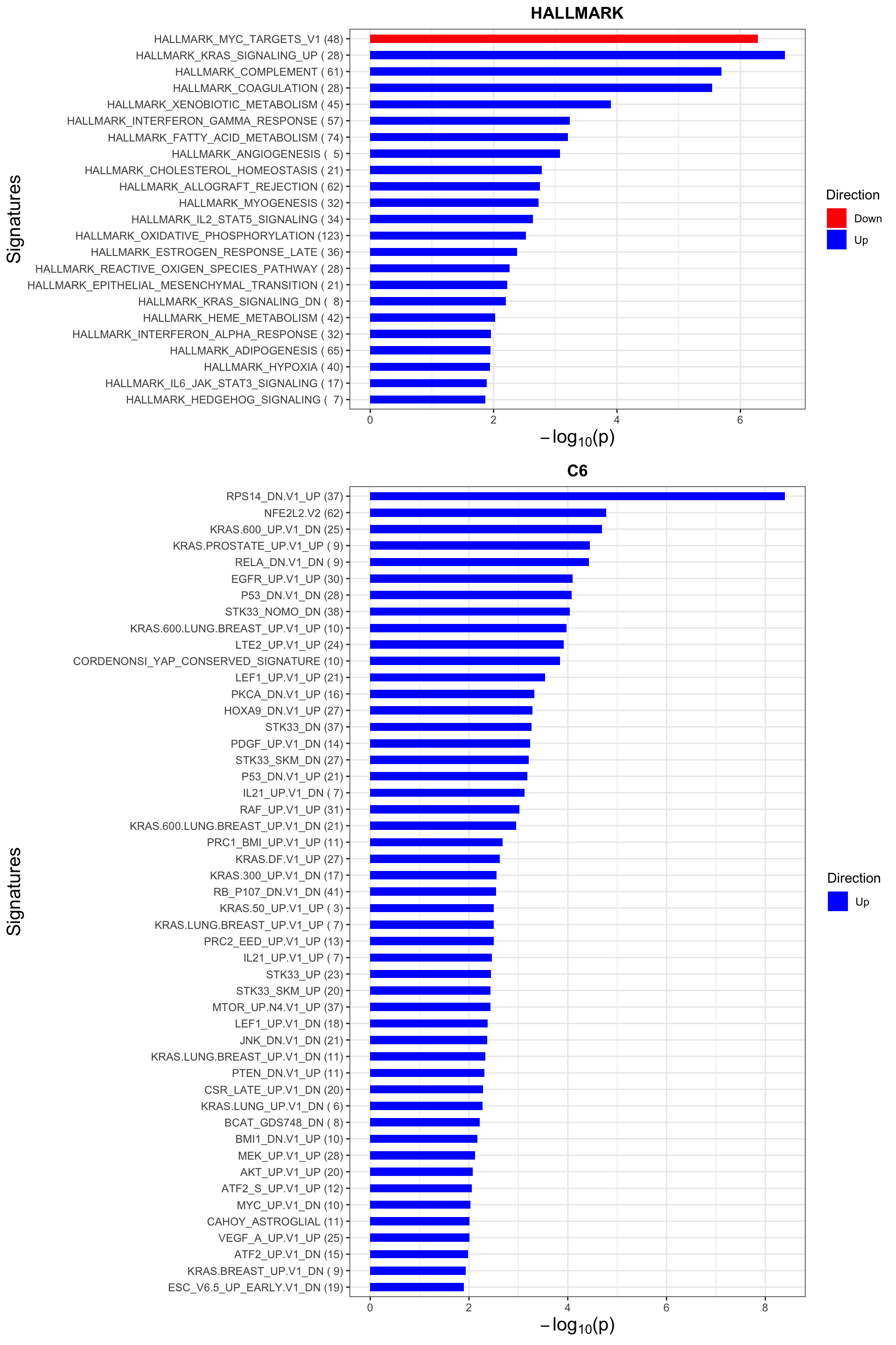
| Version | Author | Date |
|---|---|---|
| 46534c2 | Junyan Lu | 2020-02-27 |
sessionInfo()R version 3.6.0 (2019-04-26)
Platform: x86_64-apple-darwin15.6.0 (64-bit)
Running under: macOS Mojave 10.14.6
Matrix products: default
BLAS: /Library/Frameworks/R.framework/Versions/3.6/Resources/lib/libRblas.0.dylib
LAPACK: /Library/Frameworks/R.framework/Versions/3.6/Resources/lib/libRlapack.dylib
locale:
[1] en_US.UTF-8/en_US.UTF-8/en_US.UTF-8/C/en_US.UTF-8/en_US.UTF-8
attached base packages:
[1] parallel stats4 stats graphics grDevices utils datasets
[8] methods base
other attached packages:
[1] piano_2.0.2 Vennerable_3.1.0.9000
[3] forcats_0.4.0 stringr_1.4.0
[5] dplyr_0.8.3 purrr_0.3.3
[7] readr_1.3.1 tidyr_1.0.0
[9] tibble_2.1.3 ggplot2_3.2.1
[11] tidyverse_1.3.0 jyluMisc_0.1.5
[13] SummarizedExperiment_1.14.0 DelayedArray_0.10.0
[15] BiocParallel_1.18.0 matrixStats_0.54.0
[17] Biobase_2.44.0 GenomicRanges_1.36.0
[19] GenomeInfoDb_1.20.0 IRanges_2.18.1
[21] S4Vectors_0.22.0 BiocGenerics_0.30.0
loaded via a namespace (and not attached):
[1] readxl_1.3.1 backports_1.1.4 fastmatch_1.1-0
[4] drc_3.0-1 workflowr_1.6.0 plyr_1.8.4
[7] igraph_1.2.4.1 lazyeval_0.2.2 shinydashboard_0.7.1
[10] splines_3.6.0 TH.data_1.0-10 digest_0.6.19
[13] htmltools_0.3.6 gdata_2.18.0 magrittr_1.5
[16] cluster_2.1.0 openxlsx_4.1.0.1 limma_3.40.2
[19] modelr_0.1.5 sandwich_2.5-1 colorspace_1.4-1
[22] rvest_0.3.5 haven_2.2.0 xfun_0.8
[25] crayon_1.3.4 RCurl_1.95-4.12 jsonlite_1.6
[28] graph_1.62.0 zeallot_0.1.0 survival_2.44-1.1
[31] zoo_1.8-6 glue_1.3.1 survminer_0.4.4
[34] gtable_0.3.0 zlibbioc_1.30.0 XVector_0.24.0
[37] car_3.0-3 abind_1.4-5 scales_1.0.0
[40] mvtnorm_1.0-11 DBI_1.0.0 relations_0.6-8
[43] Rcpp_1.0.1 plotrix_3.7-6 xtable_1.8-4
[46] cmprsk_2.2-8 foreign_0.8-71 km.ci_0.5-2
[49] DT_0.7 htmlwidgets_1.3 httr_1.4.1
[52] fgsea_1.10.0 RColorBrewer_1.1-2 gplots_3.0.1.1
[55] ellipsis_0.2.0 pkgconfig_2.0.2 dbplyr_1.4.2
[58] labeling_0.3 reshape2_1.4.3 tidyselect_0.2.5
[61] rlang_0.4.1 later_0.8.0 munsell_0.5.0
[64] cellranger_1.1.0 tools_3.6.0 visNetwork_2.0.7
[67] cli_1.1.0 generics_0.0.2 broom_0.5.2
[70] evaluate_0.14 yaml_2.2.0 knitr_1.23
[73] fs_1.3.1 zip_2.0.2 survMisc_0.5.5
[76] caTools_1.17.1.2 RBGL_1.60.0 nlme_3.1-140
[79] whisker_0.3-2 mime_0.7 slam_0.1-45
[82] xml2_1.2.2 compiler_3.6.0 rstudioapi_0.10
[85] curl_3.3 ggsignif_0.5.0 marray_1.62.0
[88] reprex_0.3.0 stringi_1.4.3 lattice_0.20-38
[91] Matrix_1.2-17 shinyjs_1.0 KMsurv_0.1-5
[94] vctrs_0.2.0 pillar_1.4.2 lifecycle_0.1.0
[97] data.table_1.12.2 cowplot_0.9.4 bitops_1.0-6
[100] httpuv_1.5.1 R6_2.4.0 promises_1.0.1
[103] KernSmooth_2.23-15 gridExtra_2.3 rio_0.5.16
[106] codetools_0.2-16 MASS_7.3-51.4 gtools_3.8.1
[109] exactRankTests_0.8-30 assertthat_0.2.1 rprojroot_1.3-2
[112] withr_2.1.2 multcomp_1.4-10 GenomeInfoDbData_1.2.1
[115] hms_0.5.2 grid_3.6.0 rmarkdown_1.13
[118] carData_3.0-2 git2r_0.26.1 maxstat_0.7-25
[121] ggpubr_0.2.1 sets_1.0-18 shiny_1.3.2
[124] lubridate_1.7.4