Compare the results of differentially expressed genes/proteins detected in RNAseq and proteomics dataset
Junyan Lu
2020-03-07
Last updated: 2020-04-15
Checks: 6 1
Knit directory: Proteomics/analysis/
This reproducible R Markdown analysis was created with workflowr (version 1.6.0). The Checks tab describes the reproducibility checks that were applied when the results were created. The Past versions tab lists the development history.
The R Markdown file has unstaged changes. To know which version of the R Markdown file created these results, you’ll want to first commit it to the Git repo. If you’re still working on the analysis, you can ignore this warning. When you’re finished, you can run wflow_publish to commit the R Markdown file and build the HTML.
Great job! The global environment was empty. Objects defined in the global environment can affect the analysis in your R Markdown file in unknown ways. For reproduciblity it’s best to always run the code in an empty environment.
The command set.seed(20200227) was run prior to running the code in the R Markdown file. Setting a seed ensures that any results that rely on randomness, e.g. subsampling or permutations, are reproducible.
Great job! Recording the operating system, R version, and package versions is critical for reproducibility.
Nice! There were no cached chunks for this analysis, so you can be confident that you successfully produced the results during this run.
Great job! Using relative paths to the files within your workflowr project makes it easier to run your code on other machines.
Great! You are using Git for version control. Tracking code development and connecting the code version to the results is critical for reproducibility. The version displayed above was the version of the Git repository at the time these results were generated.
Note that you need to be careful to ensure that all relevant files for the analysis have been committed to Git prior to generating the results (you can use wflow_publish or wflow_git_commit). workflowr only checks the R Markdown file, but you know if there are other scripts or data files that it depends on. Below is the status of the Git repository when the results were generated:
Ignored files:
    Ignored:    .DS_Store
    Ignored:    .Rhistory
    Ignored:    .Rproj.user/
    Ignored:    analysis/.DS_Store
    Ignored:    analysis/.Rhistory
    Ignored:    analysis/correlateGenomic_cache/
    Ignored:    analysis/correlateGenomic_noBlock_MCLL_cache/
    Ignored:    analysis/correlateGenomic_noBlock_UCLL_cache/
    Ignored:    analysis/correlateGenomic_noBlock_cache/
    Ignored:    analysis/predictOutcome_cache/
    Ignored:    data/.DS_Store
    Ignored:    output/.DS_Store

Untracked files:
    Untracked:  analysis/analysisSplicing.Rmd
    Untracked:  analysis/analysisTrisomy19.Rmd
    Untracked:  analysis/correlateGenomic_noBlock.Rmd
    Untracked:  analysis/correlateGenomic_noBlock_MCLL.Rmd
    Untracked:  analysis/correlateGenomic_noBlock_UCLL.Rmd
    Untracked:  analysis/default.css
    Untracked:  analysis/peptideValidate.Rmd
    Untracked:  analysis/processPeptides_LUMOS.Rmd
    Untracked:  analysis/style.css
    Untracked:  code/utils.R
    Untracked:  data/190909_CLL_prot_abund_med_norm.tsv
    Untracked:  data/190909_CLL_prot_abund_no_norm.tsv
    Untracked:  data/20190423_Proteom_submitted_samples_bereinigt.xlsx
    Untracked:  data/20191025_Proteom_submitted_samples_final.xlsx
    Untracked:  data/LUMOS/
    Untracked:  data/LUMOS_peptides/
    Untracked:  data/LUMOS_protAnnotation.csv
    Untracked:  data/LUMOS_protAnnotation_fix.csv
    Untracked:  data/SampleAnnotation_cleaned.xlsx
    Untracked:  data/facTab_IC50atLeast3New.RData
    Untracked:  data/gmts/
    Untracked:  data/mapEnsemble.txt
    Untracked:  data/mapSymbol.txt
    Untracked:  data/pyprophet_export_aligned.csv
    Untracked:  data/timsTOF_protAnnotation.csv
    Untracked:  output/LUMOS_processed.RData
    Untracked:  output/dxdCLL.RData
    Untracked:  output/pepCLL_lumos.RData
    Untracked:  output/pepTab_lumos.RData
    Untracked:  output/proteomic_LUMOS_20200227.RData
    Untracked:  output/proteomic_LUMOS_20200320.RData
    Untracked:  output/proteomic_timsTOF_20200227.RData
    Untracked:  output/splicingResults.RData
    Untracked:  output/timsTOF_processed.RData

Unstaged changes:
    Modified:   analysis/_site.yml
    Modified:   analysis/analysisSF3B1.Rmd
    Modified:   analysis/compareProteomicsRNAseq.Rmd
    Modified:   analysis/correlateGenomic.Rmd
    Modified:   analysis/correlateMIR.Rmd
    Modified:   analysis/correlateMethylationCluster.Rmd
    Modified:   analysis/index.Rmd
    Modified:   analysis/predictOutcome.Rmd
    Modified:   analysis/processProteomics_LUMOS.Rmd
    Modified:   analysis/qualityControl_LUMOS.Rmd
Note that any generated files, e.g. HTML, png, CSS, etc., are not included in this status report because it is ok for generated content to have uncommitted changes.
These are the previous versions of the R Markdown and HTML files. If you’ve configured a remote Git repository (see ?wflow_git_remote), click on the hyperlinks in the table below to view them.
| File | Version | Author | Date | Message |
|---|---|---|---|---|
| html | b8e0823 | Junyan Lu | 2020-03-10 | Build site. |
| Rmd | c8cb45c | Junyan Lu | 2020-03-10 | update analysis |
Detect differentiall expressed proteins
Preprocessing proteomics data
protMat <- assays(protCLL)[["count"]]Differential expression using proDA
Fit the probailistic dropout model
patAnno <- data.frame(row.names = colnames(protMat),
                      IGHV = patMeta[match(colnames(protMat),patMeta$Patient.ID),]$IGHV.status,
                      trisomy12 = patMeta[match(colnames(protMat),patMeta$Patient.ID),]$trisomy12) %>%
  mutate(IGHV = factor(IGHV, levels = c("U","M")))

fit <- proDA(protMat, design = ~ IGHV + trisomy12,
             col_data = patAnno)
diffRes.prot <- list()
diffRes.prot[["IGHV"]] <- test_diff(fit, "IGHVM")
diffRes.prot[["trisomy12"]] <- test_diff(fit, "trisomy121")Differential expression using RNAseq
Preprocessing RNAseq data
dds$diag <- patMeta[match(dds$PatID, patMeta$Patient.ID),]$diagnosis
dds <- dds[,dds$diag %in% "CLL"]
dds <- estimateSizeFactors(dds)

##filter out none protein coding genes and gene on sex chromosome
dds<-dds[rowData(dds)$biotype %in% "protein_coding",]
dds <- dds[! rowData(dds)$symbol %in% c("",NA),]

##filter out low count genes
minrs <- 100
rs  <- rowSums(counts(dds, normalized = TRUE))
dds<-dds[ rs >= minrs, ]

## Add IGHV and trisomy12 annotation
dds$IGHV <- factor(patMeta[match(dds$PatID, patMeta$Patient.ID),]$IGHV.status, levels = c("U","M"))
dds$trisomy12 <- patMeta[match(dds$PatID, patMeta$Patient.ID),]$trisomy12
dds <- dds[,!(is.na(dds$IGHV) | is.na(dds$trisomy12))]

## A down-sampled data with only patients inluced in proteomic data
ddsSub <- dds[,dds$PatID %in% colnames(protMat)]
minrs <- 100
rs  <- rowSums(counts(ddsSub, normalized = TRUE))
ddsSub<-ddsSub[ rs >= minrs, ]
Differential expression using DESeq2
Full expression matrix
Test using DESeq2
dim(dds)[1] 16141 208design(dds) <- ~ IGHV + trisomy12
ddsDE <- DESeq(dds)using pre-existing size factorsestimating dispersionsgene-wise dispersion estimatesmean-dispersion relationshipfinal dispersion estimatesfitting model and testing-- replacing outliers and refitting for 692 genes
-- DESeq argument 'minReplicatesForReplace' = 7
-- original counts are preserved in counts(dds)estimating dispersionsfitting model and testingGet results
diffRes.rna <- list()
diffRes.rna[["IGHV"]] <- results(ddsDE, name = "IGHV_M_vs_U", tidy = TRUE)
diffRes.rna[["trisomy12"]] <- results(ddsDE, name = "trisomy12_1_vs_0", tidy = TRUE)
Subsetted expression matrix
Test using DESeq2
dim(ddsSub)[1] 14902 46design(ddsSub) <- ~ IGHV + trisomy12
ddsSubDE <- DESeq(ddsSub)using pre-existing size factorsestimating dispersionsgene-wise dispersion estimatesmean-dispersion relationshipfinal dispersion estimatesfitting model and testing-- replacing outliers and refitting for 473 genes
-- DESeq argument 'minReplicatesForReplace' = 7
-- original counts are preserved in counts(dds)estimating dispersionsfitting model and testingGet results
diffRes.rnaSub <- list()
diffRes.rnaSub[["IGHV"]] <- results(ddsSubDE, name = "IGHV_M_vs_U", tidy = TRUE)
diffRes.rnaSub[["trisomy12"]] <- results(ddsSubDE, name = "trisomy12_1_vs_0", tidy = TRUE)
Compare the results from proteomics and full RNAseq dataset
IGHV
Process differential expression output
protRes <- diffRes.prot$IGHV %>% mutate(symbol = rowData(protCLL_raw[name,])$hgnc_symbol) %>%
  select(symbol, pval, adj_pval, diff) %>%
  dplyr::rename(pval.prot = pval, padj.prot = adj_pval, diff.prot = diff) %>%
  arrange(pval.prot) %>% distinct(symbol, .keep_all = TRUE)

rnaRes <- diffRes.rna$IGHV %>% mutate(symbol = rowData(dds[row,])$symbol) %>%
  select(symbol, pvalue, padj, log2FoldChange) %>%
  dplyr::rename(pval.rna = pvalue, padj.rna = padj, diff.rna = log2FoldChange) %>%
  arrange(pval.rna) %>% distinct(symbol, .keep_all = TRUE)
P-value correlation plot
compareTab <- left_join(protRes, rnaRes, by = "symbol") %>%
  filter(!is.na(pval.rna)) %>%
  mutate(significant = case_when(
    padj.rna < 0.01 & padj.prot < 0.01 ~ "both",
    padj.rna < 0.01 & padj.prot >= 0.01 ~ "rnaOnly",
    padj.rna >= 0.01 & padj.prot < 0.01 ~ "proteinOnly",
    padj.rna >= 0.01 & padj.prot >= 0.01 ~"none"
  ))
ggplot(compareTab, aes(x=-log10(padj.rna),y=-log10(padj.prot))) + geom_point(aes(col = significant)) +
  scale_color_manual(values = c(both = "green",rnaOnly = "red", proteinOnly = "blue",none="grey")) +
  scale_x_log10() +
  ggrepel::geom_text_repel(data = filter(compareTab, significant == "proteinOnly"), aes(label = symbol)) +
  ylab("-log10(adjusted p value) in proteomic data") +
  xlab("-log10(adjusted p value) in RNAseq data")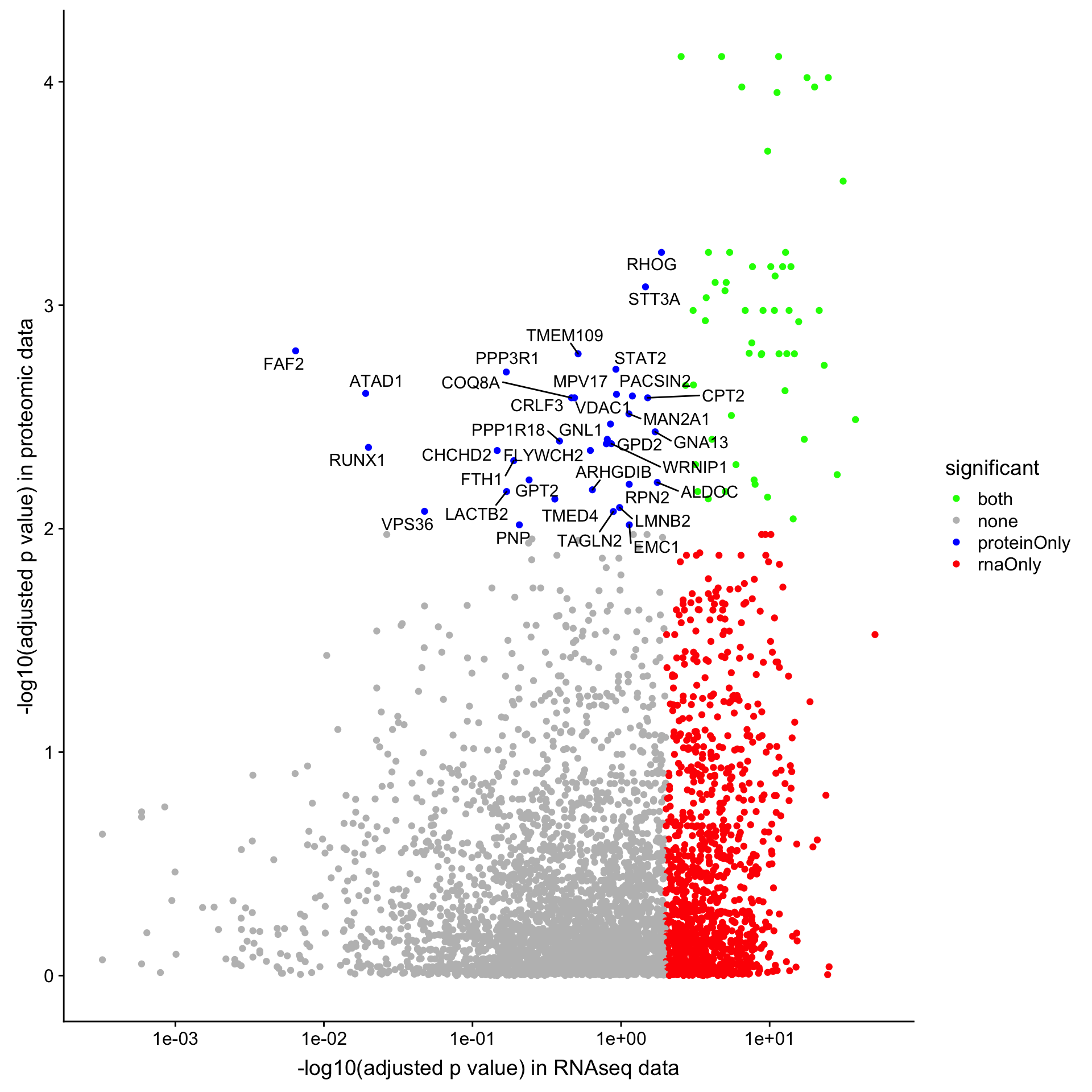
| Version | Author | Date |
|---|---|---|
| b8e0823 | Junyan Lu | 2020-03-10 |
Note that the xaxis is shown is log10 scale, to concentrate more on the differentially expressed proteins, as there are way more differentially expressed genes by RNAseq than proteins.
Upset plot (1% FDR)
upsetList <- list(RNA_up = filter(rnaRes, padj.rna <= 0.01, diff.rna > 0)$symbol,
                  RNA_down = filter(rnaRes, padj.rna <= 0.01, diff.rna < 0)$symbol,
                  Protein_up = filter(protRes, padj.prot <= 0.01, diff.prot > 0)$symbol,
                  Protein_down = filter(protRes, padj.prot <= 0.01, diff.prot < 0)$symbol)
UpSetR::upset(fromList(upsetList))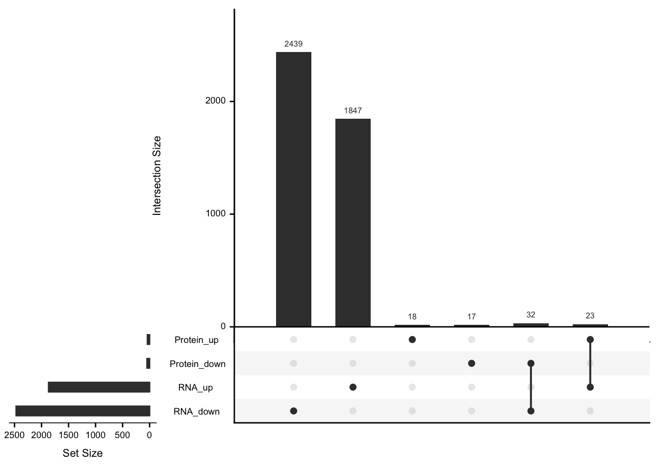
| Version | Author | Date |
|---|---|---|
| b8e0823 | Junyan Lu | 2020-03-10 |
Table of results (1% FDR)
compareTab %>% filter(significant != "none") %>%
  mutate_if(is.numeric, formatC, format ="e", digits=2) %>%
  DT::datatable(filter = "top")
trisomy12
Process differential expression output
protRes <- diffRes.prot$trisomy12 %>% mutate(symbol = rowData(protCLL_raw[name,])$hgnc_symbol) %>%
  select(symbol, pval, adj_pval, diff) %>%
  dplyr::rename(pval.prot = pval, padj.prot = adj_pval, diff.prot = diff) %>%
  arrange(pval.prot) %>% distinct(symbol, .keep_all = TRUE)

rnaRes <- diffRes.rna$trisomy12 %>% mutate(symbol = rowData(dds[row,])$symbol,
                                           chr = rowData(dds[row,])$chromosome) %>%
  select(symbol, pvalue, padj, log2FoldChange, chr) %>%
  dplyr::rename(pval.rna = pvalue, padj.rna = padj, diff.rna = log2FoldChange) %>%
  arrange(pval.rna) %>% distinct(symbol, .keep_all = TRUE)
P-value correlation plot
For all genes
compareTab <- left_join(protRes, rnaRes, by = "symbol") %>%
  filter(!is.na(pval.rna)) %>%
  mutate(significant = case_when(
    padj.rna < 0.01 & padj.prot < 0.01 ~ "both",
    padj.rna < 0.01 & padj.prot >= 0.01 ~ "rnaOnly",
    padj.rna >= 0.01 & padj.prot < 0.01 ~ "proteinOnly",
    padj.rna >= 0.01 & padj.prot >= 0.01 ~"none"
  ))
ggplot(compareTab, aes(x=-log10(padj.rna),y=-log10(padj.prot))) + geom_point(aes(col = significant)) +
  scale_color_manual(values = c(both = "green",rnaOnly = "red", proteinOnly = "blue",none="grey")) +
  scale_x_log10() +
  ggrepel::geom_text_repel(data = filter(compareTab, significant == "proteinOnly"), aes(label = symbol)) +
  ylab("-log10(adjusted p value) in proteomic data") +
  xlab("-log10(adjusted p value) in RNAseq data")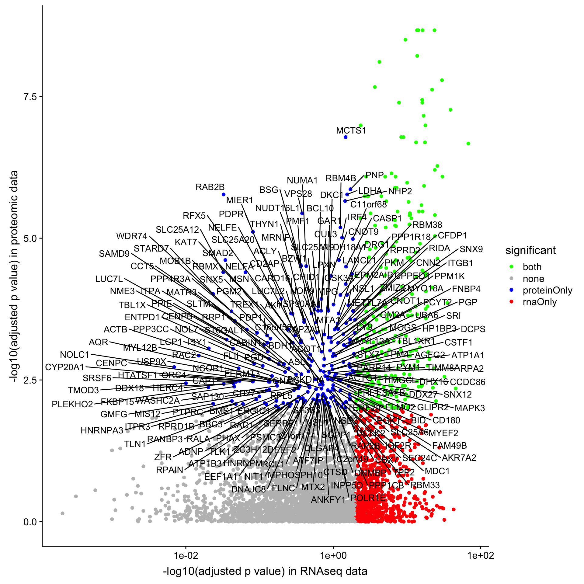
| Version | Author | Date |
|---|---|---|
| b8e0823 | Junyan Lu | 2020-03-10 |
Note that the xaxis is shown is log10 scale, to concentrate more on the differentially expressed proteins, as there are way more differentially expressed genes by RNAseq than proteins.
For genes not on chr12
plotTab <- filter(compareTab, chr != "12")
ggplot(plotTab, aes(x=-log10(padj.rna),y=-log10(padj.prot))) + geom_point(aes(col = significant)) +
  scale_color_manual(values = c(both = "green",rnaOnly = "red", proteinOnly = "blue",none="grey")) +
  scale_x_log10() +
  ggrepel::geom_text_repel(data = filter(plotTab, significant == "proteinOnly"), aes(label = symbol)) +
  ylab("-log10(adjusted p value) in proteomic data") +
  xlab("-log10(adjusted p value) in RNAseq data")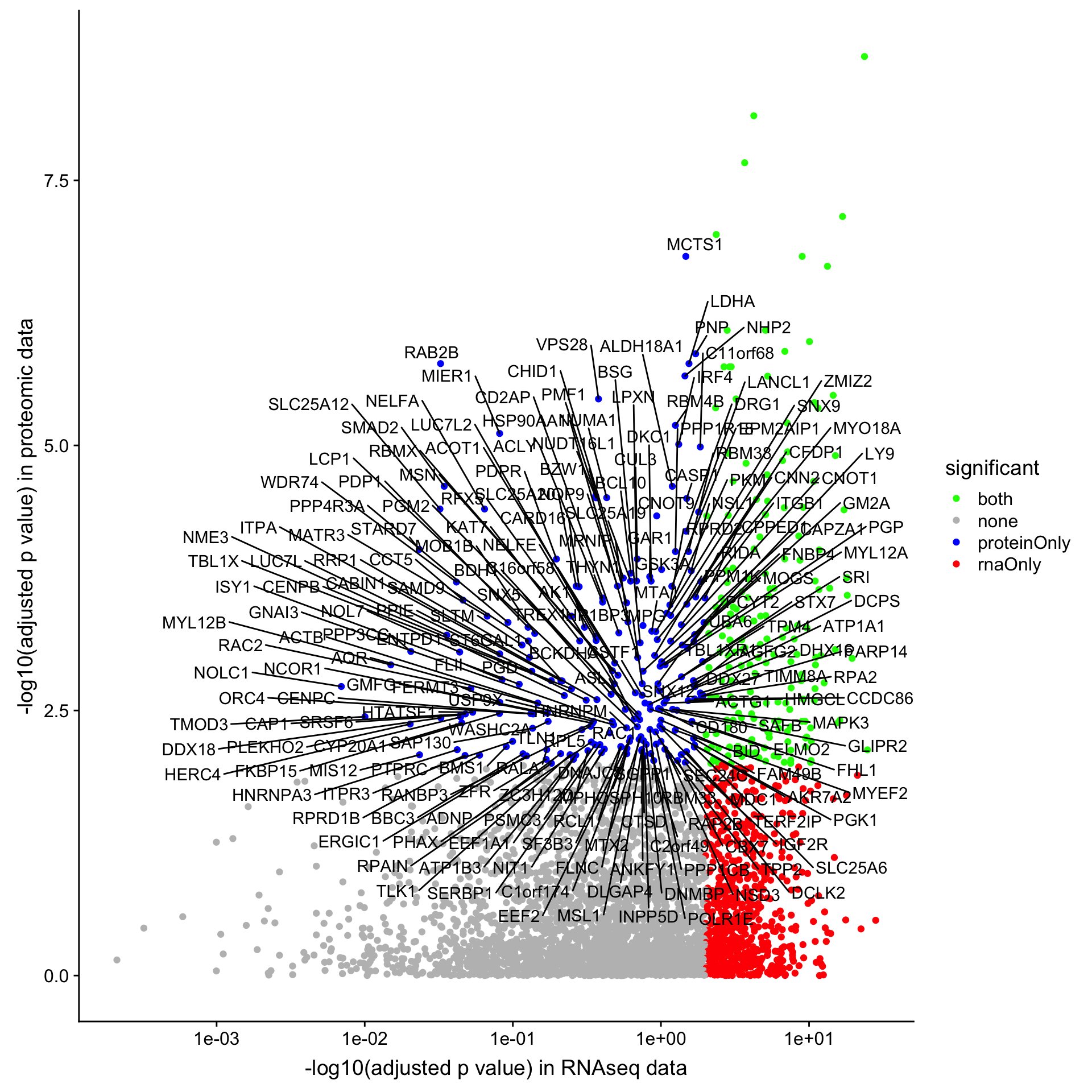
| Version | Author | Date |
|---|---|---|
| b8e0823 | Junyan Lu | 2020-03-10 |
Note that the xaxis is shown is log10 scale, to concentrate more on the differentially expressed proteins, as there are way more differentially expressed genes by RNAseq than proteins.
For genes on chr12
plotTab <- filter(compareTab, chr == "12")
ggplot(plotTab, aes(x=-log10(padj.rna),y=-log10(padj.prot))) + geom_point(aes(col = significant)) +
  scale_color_manual(values = c(both = "green",rnaOnly = "red", proteinOnly = "blue",none="grey")) +
  scale_x_log10() +
  ggrepel::geom_text_repel(data = filter(plotTab, significant == "proteinOnly"), aes(label = symbol)) +
  ylab("-log10(adjusted p value) in proteomic data") +
  xlab("-log10(adjusted p value) in RNAseq data")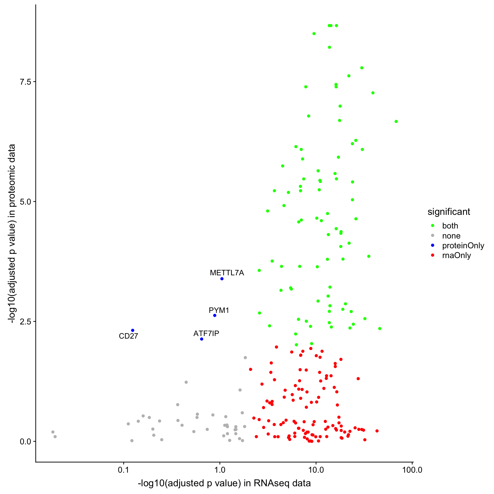
| Version | Author | Date |
|---|---|---|
| b8e0823 | Junyan Lu | 2020-03-10 |
Upset plot (1% FDR)
upsetList <- list(RNA_up = filter(rnaRes, padj.rna <= 0.01, diff.rna > 0)$symbol,
                  RNA_down = filter(rnaRes, padj.rna <= 0.01, diff.rna < 0)$symbol,
                  Protein_up = filter(protRes, padj.prot <= 0.01, diff.prot > 0)$symbol,
                  Protein_down = filter(protRes, padj.prot <= 0.01, diff.prot < 0)$symbol)
UpSetR::upset(fromList(upsetList))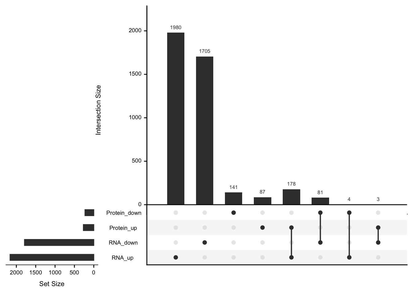
| Version | Author | Date |
|---|---|---|
| b8e0823 | Junyan Lu | 2020-03-10 |
Table of results (1% FDR)
compareTab %>% filter(significant != "none") %>%
  mutate_if(is.numeric, formatC, format ="e", digits=2) %>%
  DT::datatable(filter="top")
Compare the results from proteomics and subsetted RNAseq dataset
Only the RNAseq samples with proteomic data are included, for a fair comparison.
IGHV
Process differential expression output
protRes <- diffRes.prot$IGHV %>% mutate(symbol = rowData(protCLL_raw[name,])$hgnc_symbol) %>%
  select(symbol, pval, adj_pval, diff) %>%
  dplyr::rename(pval.prot = pval, padj.prot = adj_pval, diff.prot = diff) %>%
  arrange(pval.prot) %>% distinct(symbol, .keep_all = TRUE)

rnaRes <- diffRes.rnaSub$IGHV %>% mutate(symbol = rowData(dds[row,])$symbol) %>%
  select(symbol, pvalue, padj, log2FoldChange) %>%
  dplyr::rename(pval.rna = pvalue, padj.rna = padj, diff.rna = log2FoldChange) %>%
  arrange(pval.rna) %>% distinct(symbol, .keep_all = TRUE)
P-value correlation plot
compareTab <- left_join(protRes, rnaRes, by = "symbol") %>%
  filter(!is.na(pval.rna)) %>%
  mutate(significant = case_when(
    padj.rna < 0.01 & padj.prot < 0.01 ~ "both",
    padj.rna < 0.01 & padj.prot >= 0.01 ~ "rnaOnly",
    padj.rna >= 0.01 & padj.prot < 0.01 ~ "proteinOnly",
    padj.rna >= 0.01 & padj.prot >= 0.01 ~"none"
  ))
ggplot(compareTab, aes(x=-log10(padj.rna),y=-log10(padj.prot))) + geom_point(aes(col = significant)) +
  scale_color_manual(values = c(both = "green",rnaOnly = "red", proteinOnly = "blue",none="grey")) +
  scale_x_log10() +
  ggrepel::geom_text_repel(data = filter(compareTab, significant == "proteinOnly"), aes(label = symbol)) +
  ylab("-log10(adjusted p value) in proteomic data") +
  xlab("-log10(adjusted p value) in RNAseq data")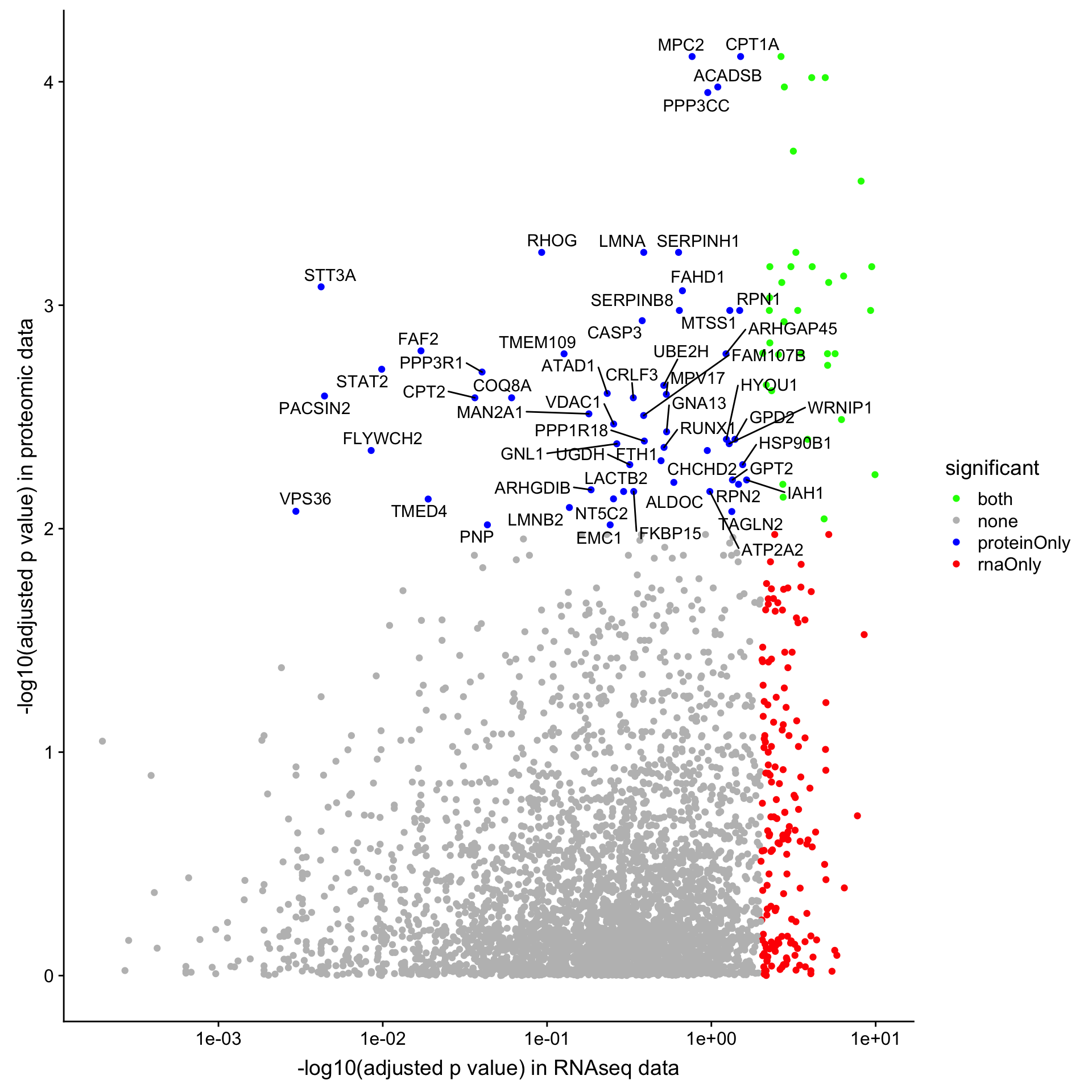
| Version | Author | Date |
|---|---|---|
| b8e0823 | Junyan Lu | 2020-03-10 |
Upset plot (1% FDR)
upsetList <- list(RNA_up = filter(rnaRes, padj.rna <= 0.01, diff.rna > 0)$symbol,
                  RNA_down = filter(rnaRes, padj.rna <= 0.01, diff.rna < 0)$symbol,
                  Protein_up = filter(protRes, padj.prot <= 0.01, diff.prot > 0)$symbol,
                  Protein_down = filter(protRes, padj.prot <= 0.01, diff.prot < 0)$symbol)
UpSetR::upset(fromList(upsetList))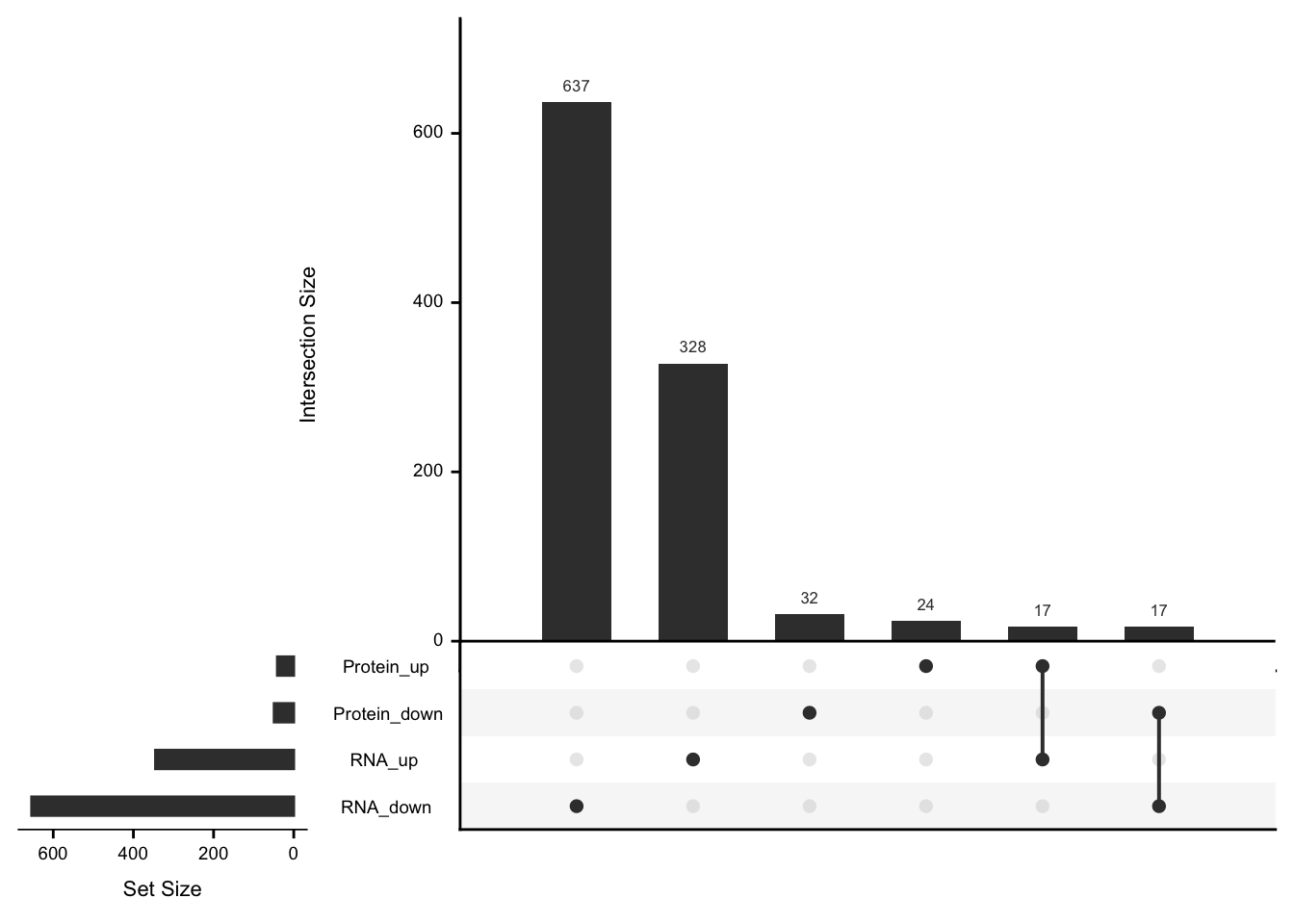
| Version | Author | Date |
|---|---|---|
| b8e0823 | Junyan Lu | 2020-03-10 |
RNAseq still detects more differentially expressed genes
Table of results (1% FDR)
compareTab %>% filter(significant != "none") %>%
  mutate_if(is.numeric, formatC, format ="e", digits=2) %>%
  DT::datatable(filter = "top")
trisomy12
Process differential expression output
protRes <- diffRes.prot$trisomy12 %>% mutate(symbol = rowData(protCLL_raw[name,])$hgnc_symbol) %>%
  select(symbol, pval, adj_pval, diff) %>%
  dplyr::rename(pval.prot = pval, padj.prot = adj_pval, diff.prot = diff) %>%
  arrange(pval.prot) %>% distinct(symbol, .keep_all = TRUE)

rnaRes <- diffRes.rnaSub$trisomy12 %>% mutate(symbol = rowData(dds[row,])$symbol,
                                           chr = rowData(dds[row,])$chromosome) %>%
  select(symbol, pvalue, padj, log2FoldChange, chr) %>%
  dplyr::rename(pval.rna = pvalue, padj.rna = padj, diff.rna = log2FoldChange) %>%
  arrange(pval.rna) %>% distinct(symbol, .keep_all = TRUE)
P-value correlation plot
For all genes
compareTab <- left_join(protRes, rnaRes, by = "symbol") %>%
  filter(!is.na(pval.rna)) %>%
  mutate(significant = case_when(
    padj.rna < 0.01 & padj.prot < 0.01 ~ "both",
    padj.rna < 0.01 & padj.prot >= 0.01 ~ "rnaOnly",
    padj.rna >= 0.01 & padj.prot < 0.01 ~ "proteinOnly",
    padj.rna >= 0.01 & padj.prot >= 0.01 ~"none"
  ))
ggplot(compareTab, aes(x=-log10(padj.rna),y=-log10(padj.prot))) + geom_point(aes(col = significant)) +
  scale_color_manual(values = c(both = "green",rnaOnly = "red", proteinOnly = "blue",none="grey")) +
  scale_x_log10() +
  ggrepel::geom_text_repel(data = filter(compareTab, significant == "proteinOnly"), aes(label = symbol)) +
  ylab("-log10(adjusted p value) in proteomic data") +
  xlab("-log10(adjusted p value) in RNAseq data")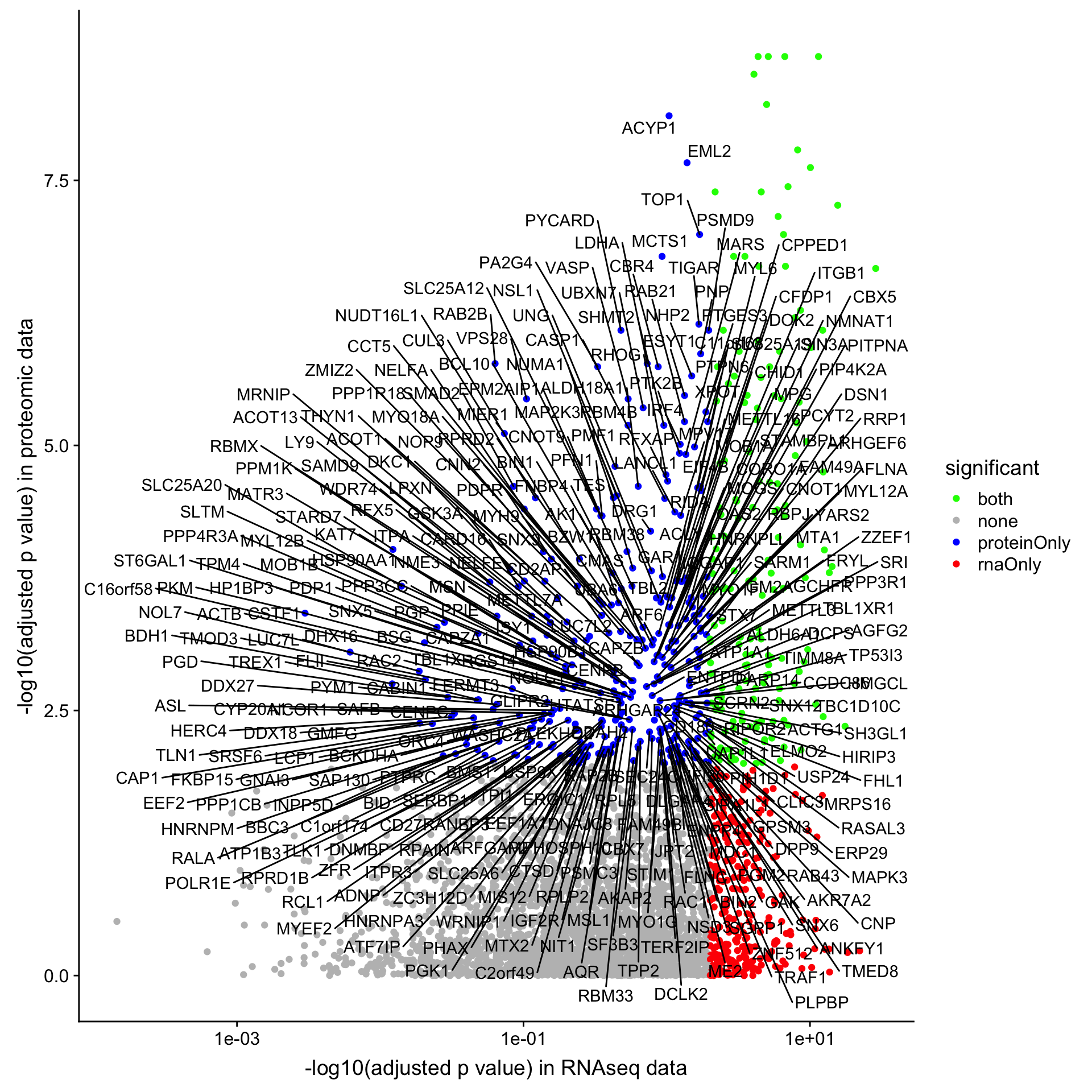
| Version | Author | Date |
|---|---|---|
| b8e0823 | Junyan Lu | 2020-03-10 |
Note that the xaxis is shown is log10 scale, to concentrate more on the differentially expressed proteins, as there are way more differentially expressed genes by RNAseq than proteins.
For genes not on chr12
plotTab <- filter(compareTab, chr != "12")
ggplot(plotTab, aes(x=-log10(padj.rna),y=-log10(padj.prot))) + geom_point(aes(col = significant)) +
  scale_color_manual(values = c(both = "green",rnaOnly = "red", proteinOnly = "blue",none="grey")) +
  scale_x_log10() +
  ggrepel::geom_text_repel(data = filter(plotTab, significant == "proteinOnly"), aes(label = symbol)) +
  ylab("-log10(adjusted p value) in proteomic data") +
  xlab("-log10(adjusted p value) in RNAseq data")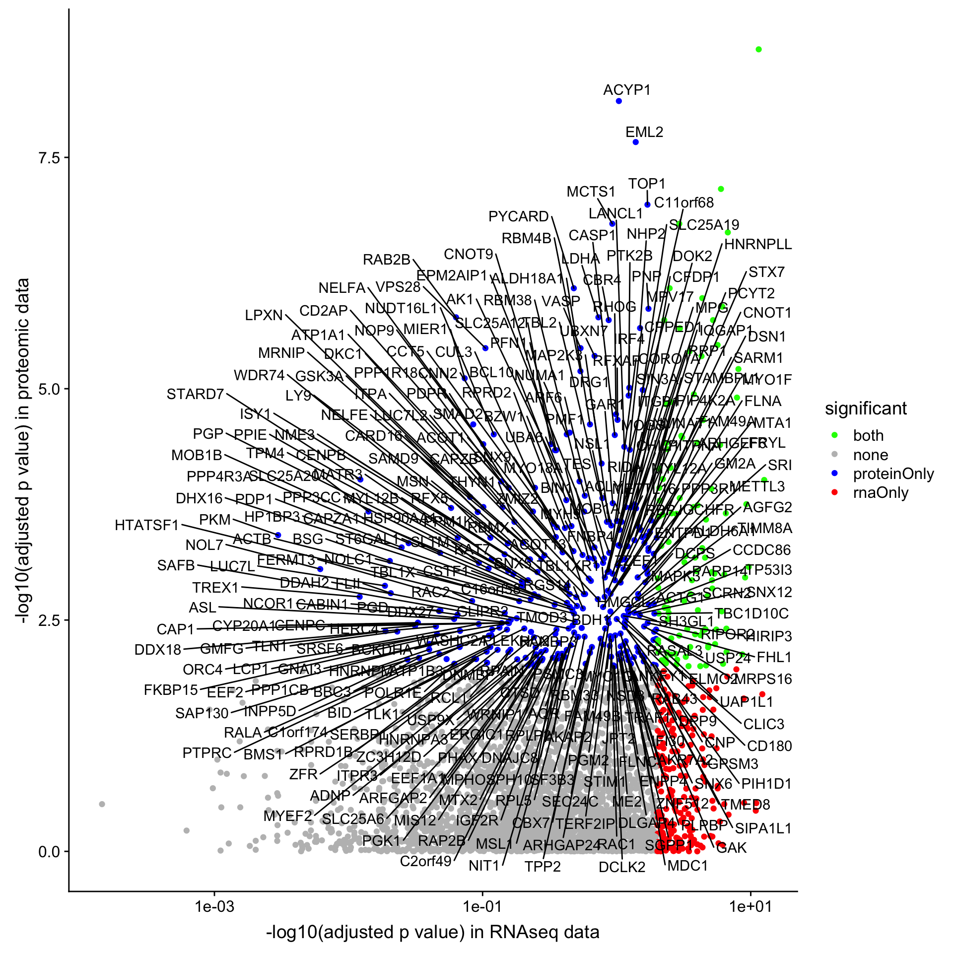
| Version | Author | Date |
|---|---|---|
| b8e0823 | Junyan Lu | 2020-03-10 |
Note that the xaxis is shown is log10 scale, to concentrate more on the differentially expressed proteins, as there are way more differentially expressed genes by RNAseq than proteins.
For genes on chr12
plotTab <- filter(compareTab, chr == "12")
ggplot(plotTab, aes(x=-log10(padj.rna),y=-log10(padj.prot))) + geom_point(aes(col = significant)) +
  scale_color_manual(values = c(both = "green",rnaOnly = "red", proteinOnly = "blue",none="grey")) +
  scale_x_log10() +
  ggrepel::geom_text_repel(data = filter(plotTab, significant == "proteinOnly"), aes(label = symbol)) +
  ylab("-log10(adjusted p value) in proteomic data") +
  xlab("-log10(adjusted p value) in RNAseq data")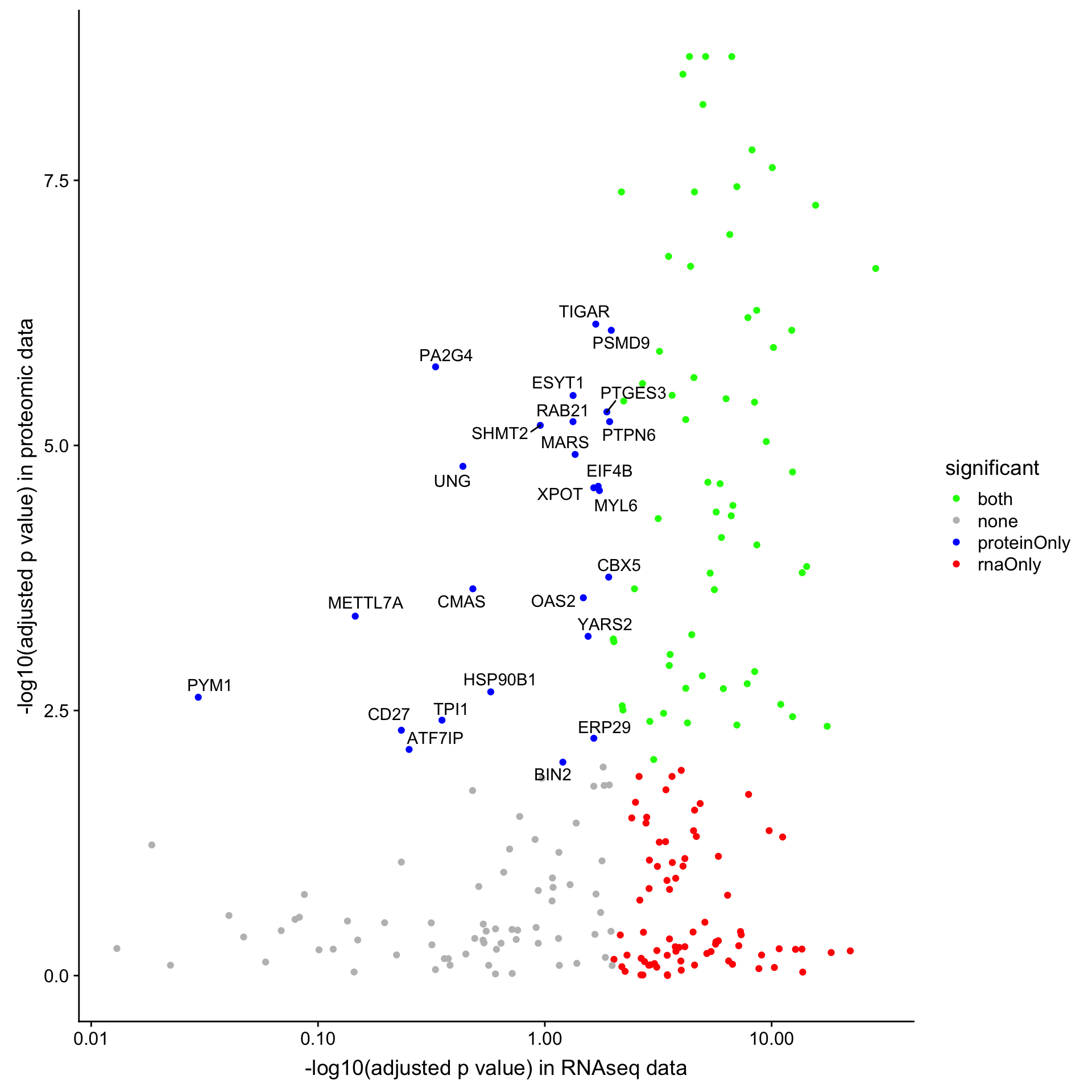
| Version | Author | Date |
|---|---|---|
| b8e0823 | Junyan Lu | 2020-03-10 |
Upset plot (1% FDR)
upsetList <- list(RNA_up = filter(rnaRes, padj.rna <= 0.01, diff.rna > 0)$symbol,
                  RNA_down = filter(rnaRes, padj.rna <= 0.01, diff.rna < 0)$symbol,
                  Protein_up = filter(protRes, padj.prot <= 0.01, diff.prot > 0)$symbol,
                  Protein_down = filter(protRes, padj.prot <= 0.01, diff.prot < 0)$symbol)
UpSetR::upset(fromList(upsetList))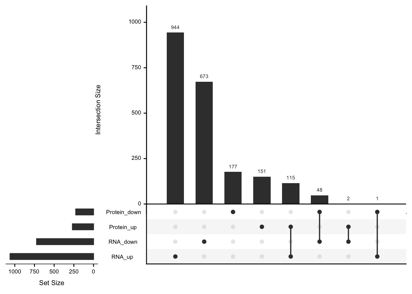
| Version | Author | Date |
|---|---|---|
| b8e0823 | Junyan Lu | 2020-03-10 |
Table of results (1% FDR)
compareTab %>% filter(significant != "none") %>%
  mutate_if(is.numeric, formatC, format ="e", digits=2) %>%
  DT::datatable(filter="top")
sessionInfo()R version 3.6.0 (2019-04-26)
Platform: x86_64-apple-darwin15.6.0 (64-bit)
Running under: macOS 10.15.3
Matrix products: default
BLAS: /Library/Frameworks/R.framework/Versions/3.6/Resources/lib/libRblas.0.dylib
LAPACK: /Library/Frameworks/R.framework/Versions/3.6/Resources/lib/libRlapack.dylib
locale:
[1] en_US.UTF-8/en_US.UTF-8/en_US.UTF-8/C/en_US.UTF-8/en_US.UTF-8
attached base packages:
[1] parallel stats4 stats graphics grDevices utils datasets
[8] methods base
other attached packages:
[1] forcats_0.4.0 stringr_1.4.0
[3] dplyr_0.8.5 purrr_0.3.3
[5] readr_1.3.1 tidyr_1.0.0
[7] tibble_3.0.0 tidyverse_1.3.0
[9] jyluMisc_0.1.5 ggrepel_0.8.1
[11] proDA_1.1.2 UpSetR_1.4.0
[13] vsn_3.52.0 DESeq2_1.24.0
[15] SummarizedExperiment_1.14.0 DelayedArray_0.10.0
[17] BiocParallel_1.18.0 matrixStats_0.54.0
[19] Biobase_2.44.0 GenomicRanges_1.36.0
[21] GenomeInfoDb_1.20.0 IRanges_2.18.1
[23] S4Vectors_0.22.0 BiocGenerics_0.30.0
[25] cowplot_0.9.4 ggplot2_3.3.0
[27] limma_3.40.2
loaded via a namespace (and not attached):
[1] shinydashboard_0.7.1 tidyselect_1.0.0 RSQLite_2.1.1
[4] AnnotationDbi_1.46.0 htmlwidgets_1.3 grid_3.6.0
[7] maxstat_0.7-25 munsell_0.5.0 codetools_0.2-16
[10] preprocessCore_1.46.0 DT_0.7 withr_2.1.2
[13] colorspace_1.4-1 knitr_1.23 rstudioapi_0.10
[16] ggsignif_0.5.0 labeling_0.3 git2r_0.26.1
[19] slam_0.1-45 GenomeInfoDbData_1.2.1 KMsurv_0.1-5
[22] farver_2.0.3 bit64_0.9-7 rprojroot_1.3-2
[25] vctrs_0.2.4 generics_0.0.2 TH.data_1.0-10
[28] xfun_0.8 sets_1.0-18 R6_2.4.0
[31] locfit_1.5-9.1 bitops_1.0-6 fgsea_1.10.0
[34] assertthat_0.2.1 promises_1.0.1 scales_1.1.0
[37] multcomp_1.4-10 nnet_7.3-12 gtable_0.3.0
[40] extraDistr_1.8.11 affy_1.62.0 sandwich_2.5-1
[43] workflowr_1.6.0 rlang_0.4.5 genefilter_1.66.0
[46] cmprsk_2.2-8 splines_3.6.0 acepack_1.4.1
[49] broom_0.5.2 checkmate_2.0.0 BiocManager_1.30.4
[52] yaml_2.2.0 abind_1.4-5 modelr_0.1.5
[55] crosstalk_1.0.0 backports_1.1.4 httpuv_1.5.1
[58] Hmisc_4.2-0 tools_3.6.0 relations_0.6-8
[61] affyio_1.54.0 ellipsis_0.2.0 gplots_3.0.1.1
[64] RColorBrewer_1.1-2 Rcpp_1.0.1 plyr_1.8.4
[67] base64enc_0.1-3 visNetwork_2.0.7 zlibbioc_1.30.0
[70] RCurl_1.95-4.12 ggpubr_0.2.1 rpart_4.1-15
[73] zoo_1.8-6 haven_2.2.0 cluster_2.1.0
[76] exactRankTests_0.8-30 fs_1.4.0 magrittr_1.5
[79] data.table_1.12.2 openxlsx_4.1.0.1 reprex_0.3.0
[82] survminer_0.4.4 mvtnorm_1.0-11 whisker_0.3-2
[85] hms_0.5.2 shinyjs_1.0 mime_0.7
[88] evaluate_0.14 xtable_1.8-4 XML_3.98-1.20
[91] rio_0.5.16 readxl_1.3.1 gridExtra_2.3
[94] compiler_3.6.0 KernSmooth_2.23-15 crayon_1.3.4
[97] htmltools_0.4.0 later_0.8.0 Formula_1.2-3
[100] geneplotter_1.62.0 lubridate_1.7.4 DBI_1.0.0
[103] dbplyr_1.4.2 MASS_7.3-51.4 Matrix_1.2-17
[106] car_3.0-3 cli_1.1.0 marray_1.62.0
[109] gdata_2.18.0 igraph_1.2.4.1 pkgconfig_2.0.2
[112] km.ci_0.5-2 foreign_0.8-71 piano_2.0.2
[115] xml2_1.2.2 annotate_1.62.0 XVector_0.24.0
[118] drc_3.0-1 rvest_0.3.5 digest_0.6.19
[121] rmarkdown_1.13 cellranger_1.1.0 fastmatch_1.1-0
[124] survMisc_0.5.5 htmlTable_1.13.1 curl_3.3
[127] shiny_1.3.2 gtools_3.8.1 lifecycle_0.2.0
[130] nlme_3.1-140 jsonlite_1.6 carData_3.0-2
[133] pillar_1.4.3 lattice_0.20-38 httr_1.4.1
[136] plotrix_3.7-6 survival_2.44-1.1 glue_1.3.2
[139] zip_2.0.2 bit_1.1-14 stringi_1.4.3
[142] blob_1.1.1 latticeExtra_0.6-28 caTools_1.17.1.2
[145] memoise_1.1.0