Load libraries and dataset

library(SummarizedExperiment)
library(tidygraph)
library(DGCA)
library(proDA)
library(DESeq2)
library(cowplot)
library(igraph)
library(ggraph)
library(tidyverse)

Prepare datasets

load("../output/proteomic_LUMOS_20200430.RData")
load("../../var/patmeta_200522.RData")
load("../../var/ddsrna_180717.RData")

Preprocessing protein and RNA data

#subset samples and genes
overSampe <- intersect(colnames(dds), colnames(protCLL))
overGene <- intersect(rownames(dds), rowData(protCLL)$ensembl_gene_id)
ddsSub <- dds[overGene, overSampe]
protSub <- protCLL[match(overGene, rowData(protCLL)$ensembl_gene_id),overSampe]
rowData(ddsSub)$uniprotID <- rownames(protSub)[match(rownames(ddsSub),rowData(protSub)$ensembl_gene_id)]

#vst
ddsSub.vst <- varianceStabilizingTransformation(ddsSub)

Processing protein complex data

int_pairs <- read_delim("../data/proteins_in_complexes", delim = "\t") %>%
  mutate(Reactome = grepl("Reactome",Evidence_supporting_the_interaction),
         Corum = grepl("Corum",Evidence_supporting_the_interaction)) %>%
  filter(ProtA %in% rownames(protSub) & ProtB %in% rownames(protSub)) %>%
  mutate(pair=map2_chr(ProtA, ProtB, ~paste0(sort(c(.x,.y)), collapse = "-"))) %>%
  mutate(database = case_when(
    Reactome & Corum ~ "both",
    Reactome & !Corum ~ "Reactome",
    !Reactome & Corum ~ "Corum",
    TRUE ~ "other"
  )) %>% mutate(inComplex = "yes")

Differential protein and RNA expression analysis related to U-CLL (unmutated IGHV status)

exprMat <- assays(protCLL)[["count"]]
designMat <- data.frame(row.names  = colnames(protCLL), IGHV = protCLL$IGHV.status, trisomy12 = protCLL$trisomy12)
fit <- proDA(exprMat, design = ~ .,
             col_data = designMat)

protRes <- test_diff(fit, "IGHVU") %>%
    dplyr::rename(uniprotID = name, logFC = diff, 
                  pvalue = pval, padj = adj_pval) %>% 
    mutate(name = rowData(protCLL[uniprotID,])$hgnc_symbol,
           chrom = rowData(protCLL[uniprotID,])$chromosome_name,
           geneID = rowData(protCLL[uniprotID,])$ensembl_gene_id) %>%
    select(name, uniprotID, geneID, chrom, logFC, pvalue, padj) %>%  
    arrange(pvalue) %>% as_tibble() 

ddsSub$trisomy12 <- patMeta[match(ddsSub$PatID,patMeta$Patient.ID),]$trisomy12
ddsSub$IGHV <- patMeta[match(ddsSub$PatID, patMeta$Patient.ID),]$IGHV.status
design(ddsSub) <- ~ trisomy12 + IGHV
deRes <- DESeq(ddsSub, betaPrior = TRUE)
rnaRes <- results(deRes, name = "IGHVU", tidy = TRUE) %>%
  dplyr::rename(geneID = row, log2FC.rna = log2FoldChange, 
                pvalue.rna = pvalue, padj.rna = padj) %>%
  select(geneID, log2FC.rna, pvalue.rna, padj.rna)

allRes <- left_join(protRes, rnaRes, by = "geneID")

Construct protein-protein interaction network by “cause” proteins and “effect” proteins

fdrCut <- 0.1
resTab <- select(allRes, name, uniprotID, chrom, padj, padj.rna, logFC, log2FC.rna) %>%
  mutate(sigProt = padj <= fdrCut,
         sigRna = padj.rna <=fdrCut,
         upProt = logFC > 0,
         upRna = log2FC.rna >0)

comTab <- int_pairs %>% select(ProtA, ProtB, database) %>%
  left_join(resTab, by = c(ProtA = "uniprotID")) %>%
  left_join(resTab, by = c(ProtB = "uniprotID"))

comTab.filter <- comTab %>%
  filter(sigProt.x, sigProt.y, logFC.x*logFC.y >0) %>%
  mutate(direct = ifelse(logFC.x >0, "stabilizing", "destabilizing")) %>%
  mutate(source = case_when(
    sigProt.x & sigRna.x & sigProt.y & !sigRna.y ~ name.x,
    sigProt.y & sigRna.y & sigProt.x & !sigRna.x ~ name.y)) %>%
  filter(!is.na(source)) %>%
  mutate(target = ifelse(name.x == source, name.y, name.x)) %>%
  select(source, target, direct)

#get node list
allNodes <- union(comTab.filter$source, comTab.filter$target) 

nodeList <- data.frame(id = seq(length(allNodes))-1, name = allNodes, stringsAsFactors = FALSE) %>%
  mutate(causal = ifelse(name %in% comTab.filter$source, "cause", "effect"))

#get edge list
edgeList <- select(comTab.filter, source, target, direct) %>%
  dplyr::rename(Source = source, Target = target) %>% 
  mutate(Source = nodeList[match(Source,nodeList$name),]$id,
         Target = nodeList[match(Target, nodeList$name),]$id) %>%
  data.frame(stringsAsFactors = FALSE)

net <- graph_from_data_frame(vertices = nodeList, d=edgeList, directed = FALSE)

tidyNet <- as_tbl_graph(net)
ggraph(tidyNet) + geom_edge_link(aes(color = direct), width=1) + 
  geom_node_point(aes(color =causal, shape = causal), size=5) + 
  geom_node_text(aes(label = name), repel = TRUE) +
  scale_color_manual(values = c(cause = "red",effect = "blue")) +
  scale_edge_color_brewer(palette = "Set2") +
  theme_graph()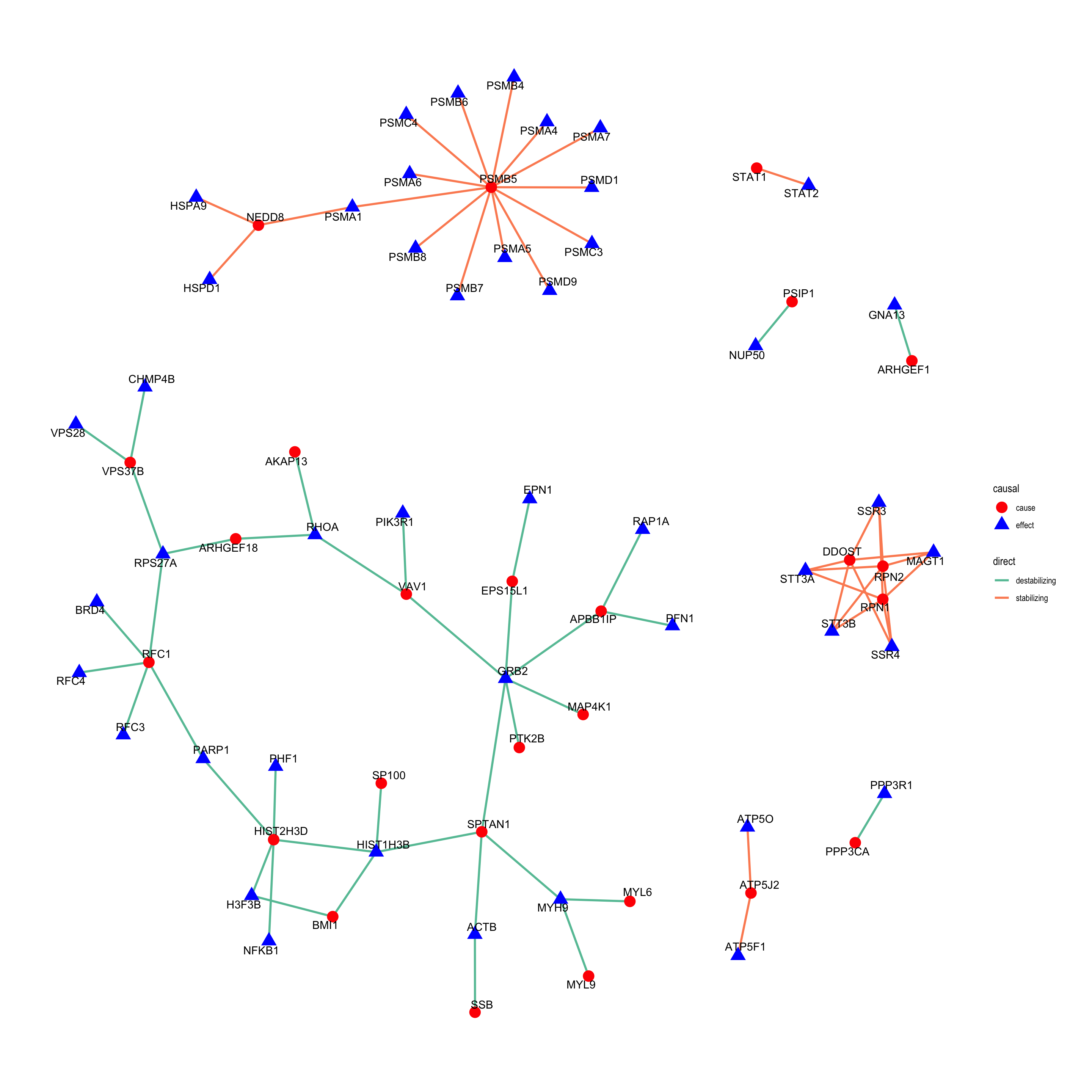 

In this plot, the “cause” proteins, which show both RNA and protein changes, are shown as red circle and the “effect” proteins, which only show protein level changes are shown as blue triangles. Different to the trisomy12 analysis, the “cause” can be up-regulated or down-regulated. Therefore, I also defined a direction of the effect, which can be “stabilizing” or “destabilizing”. Stabilizing means the “cause” protein and “effect” protein are both up-regulated, indicating that the abundance of the “effect” protein is stabilized by forming complex with a protein up-regulated by U-IGHV. While “destabilizing” means both proteins are down-regulated, indicating the “effect” protein is destabilized by the down-regulation of another protein in the complexes due to U-IGHV.

Compare to trisomy12, the network is much more sparse, which is reasonable as there are less proteins regulated by IGHV. But there are also some interesting pair. For example, GRB2, which are down-regulated in U-CLL at protein levels but not RNA levels, are connected to several proteins that are down-regulated at both RNA and protein levels in U-CLL. This can be explained as the down-regulations of those proteins leads to less protection effect to GRB2 through forming complexes in U-CLL and therefore, the protein abundance of GRB2 is decreased. On the other hand, the up-regulation of STAT1 on both RNA and protein levels seems to stabilize STAT2 in U-CLL through forming complex. Let me know if you spot other interesting cases that need further investigation.

Prepare complex table

edgeTab <- int_pairs %>% select(ProtA, ProtB, database) %>%
  mutate(chrA = rowData(protCLL[ProtA,])$chromosome_name,
         chrB = rowData(protCLL[ProtB,])$chromosome_name,
         nameA = rowData(protCLL[ProtA,])$hgnc_symbol,
         nameB = rowData(protCLL[ProtB,])$hgnc_symbol) %>%
  filter(!is.na(chrA), !is.na(chrB)) %>%
  select(ProtA, ProtB, nameA, nameB, database)

fdrCut <- 0.1
nodeTab <- select(allRes, name, uniprotID, chrom, padj, padj.rna, logFC,log2FC.rna) %>%
  mutate(sigProt = padj <= fdrCut,
         sigRna = padj.rna <=fdrCut) %>%
  mutate(changeRNA = case_when(
     sigRna & log2FC.rna > 0 ~ "Up",
     sigRna & log2FC.rna <0 ~ "Down",
     TRUE ~ "n.s."
  ),
  changeProtein = case_when(
    sigProt & logFC > 0 ~ "Up",
    sigProt & logFC < 0 ~ "Down",
    TRUE ~ "n.s."
  )) %>% select(name, chrom, changeRNA, changeProtein)

STAT1-STAT2

plotSubNet <- function(protList,edgeTab, nodeTab) {
  #get node list
  subCom <- filter(edgeTab, nameA %in% protList | nameB %in% protList)
  allNodes <- union(subCom$nameA, subCom$nameB) 
   
  nodeList <- data.frame(id = seq(length(allNodes))-1, name = allNodes, stringsAsFactors = FALSE) %>%
    left_join(nodeTab, by = "name") 
  
  #get edge list
  edgeList <- select(subCom, nameA, nameB, database) %>%
    dplyr::rename(Source = nameA, Target = nameB) %>% 
    mutate(Source = nodeList[match(Source,nodeList$name),]$id,
           Target = nodeList[match(Target, nodeList$name),]$id) %>%
    data.frame(stringsAsFactors = FALSE)
  
  net <- graph_from_data_frame(vertices = nodeList, d=edgeList, directed = FALSE)
  
  tidyNet <- as_tbl_graph(net)
ggraph(tidyNet) + geom_edge_link(aes(color = database), width=1) + 
  geom_node_point(aes(color = changeProtein, shape = changeRNA), size=5) + 
  geom_node_text(aes(label = name), repel = TRUE) +
  scale_color_manual(values = c(Up = "red", Down = "blue", n.s. = "grey")) +
  scale_edge_color_brewer(palette = "Set2") +
  theme_graph() 

}

protList <- c("STAT1","STAT2")
plotSubNet(protList, edgeTab, nodeTab)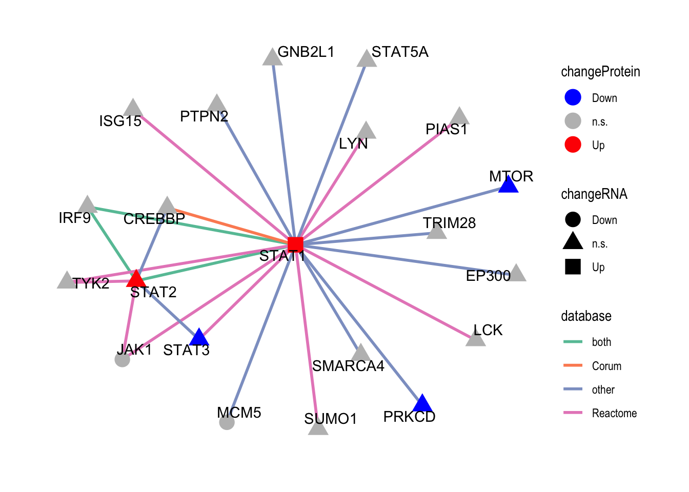

The color scheme here is a little different to the plot above or the trisomy12 network plot, because gene dosage effect is not involved and genes can be up-/down-regulated. In this plot, the color of the nodes indicates expression change at protein level, the shape of the nodes indicates expression change at RNA level.

Session information

sessionInfo()

R version 3.6.0 (2019-04-26)
Platform: x86_64-apple-darwin15.6.0 (64-bit)
Running under: macOS  10.15.4

Matrix products: default
BLAS:   /Library/Frameworks/R.framework/Versions/3.6/Resources/lib/libRblas.0.dylib
LAPACK: /Library/Frameworks/R.framework/Versions/3.6/Resources/lib/libRlapack.dylib

locale:
[1] en_US.UTF-8/en_US.UTF-8/en_US.UTF-8/C/en_US.UTF-8/en_US.UTF-8

attached base packages:
[1] parallel  stats4    stats     graphics  grDevices utils     datasets 
[8] methods   base     

other attached packages:
 [1] forcats_0.4.0               stringr_1.4.0              
 [3] dplyr_0.8.5                 purrr_0.3.3                
 [5] readr_1.3.1                 tidyr_1.0.0                
 [7] tibble_3.0.0                tidyverse_1.3.0            
 [9] ggraph_1.0.2                igraph_1.2.4.1             
[11] cowplot_0.9.4               ggplot2_3.3.0              
[13] DESeq2_1.24.0               proDA_1.1.2                
[15] DGCA_1.0.2                  tidygraph_1.1.2            
[17] SummarizedExperiment_1.14.0 DelayedArray_0.10.0        
[19] BiocParallel_1.18.0         matrixStats_0.54.0         
[21] Biobase_2.44.0              GenomicRanges_1.36.0       
[23] GenomeInfoDb_1.20.0         IRanges_2.18.1             
[25] S4Vectors_0.22.0            BiocGenerics_0.30.0        

loaded via a namespace (and not attached):
  [1] readxl_1.3.1           backports_1.1.4        Hmisc_4.2-0           
  [4] workflowr_1.6.0        plyr_1.8.4             splines_3.6.0         
  [7] robust_0.4-18.1        digest_0.6.19          foreach_1.4.4         
 [10] htmltools_0.4.0        viridis_0.5.1          GO.db_3.8.2           
 [13] magrittr_1.5           checkmate_2.0.0        memoise_1.1.0         
 [16] fit.models_0.5-14      cluster_2.1.0          doParallel_1.0.14     
 [19] fastcluster_1.1.25     annotate_1.62.0        modelr_0.1.5          
 [22] colorspace_1.4-1       rvest_0.3.5            blob_1.1.1            
 [25] rrcov_1.4-9            ggrepel_0.8.1          haven_2.2.0           
 [28] xfun_0.8               crayon_1.3.4           RCurl_1.95-4.12       
 [31] jsonlite_1.6           genefilter_1.66.0      impute_1.58.0         
 [34] survival_2.44-1.1      iterators_1.0.10       glue_1.3.2            
 [37] polyclip_1.10-0        gtable_0.3.0           zlibbioc_1.30.0       
 [40] XVector_0.24.0         DEoptimR_1.0-8         scales_1.1.0          
 [43] mvtnorm_1.0-11         DBI_1.0.0              Rcpp_1.0.1            
 [46] viridisLite_0.3.0      xtable_1.8-4           htmlTable_1.13.1      
 [49] foreign_0.8-71         bit_1.1-14             preprocessCore_1.46.0 
 [52] Formula_1.2-3          htmlwidgets_1.3        httr_1.4.1            
 [55] RColorBrewer_1.1-2     acepack_1.4.1          ellipsis_0.2.0        
 [58] pkgconfig_2.0.2        XML_3.98-1.20          farver_2.0.3          
 [61] nnet_7.3-12            dbplyr_1.4.2           locfit_1.5-9.1        
 [64] dynamicTreeCut_1.63-1  labeling_0.3           tidyselect_1.0.0      
 [67] rlang_0.4.5            later_0.8.0            AnnotationDbi_1.46.0  
 [70] cellranger_1.1.0       munsell_0.5.0          tools_3.6.0           
 [73] cli_1.1.0              generics_0.0.2         RSQLite_2.1.1         
 [76] broom_0.5.2            evaluate_0.14          yaml_2.2.0            
 [79] knitr_1.23             bit64_0.9-7            fs_1.4.0              
 [82] robustbase_0.93-5      nlme_3.1-140           xml2_1.2.2            
 [85] compiler_3.6.0         rstudioapi_0.10        reprex_0.3.0          
 [88] tweenr_1.0.1           geneplotter_1.62.0     pcaPP_1.9-73          
 [91] stringi_1.4.3          lattice_0.20-38        Matrix_1.2-17         
 [94] vctrs_0.2.4            pillar_1.4.3           lifecycle_0.2.0       
 [97] data.table_1.12.2      bitops_1.0-6           httpuv_1.5.1          
[100] R6_2.4.0               latticeExtra_0.6-28    promises_1.0.1        
[103] gridExtra_2.3          codetools_0.2-16       MASS_7.3-51.4         
[106] assertthat_0.2.1       rprojroot_1.3-2        withr_2.1.2           
[109] GenomeInfoDbData_1.2.1 hms_0.5.2              grid_3.6.0            
[112] rpart_4.1-15           rmarkdown_1.13         git2r_0.26.1          
[115] ggforce_0.2.2          lubridate_1.7.4        WGCNA_1.68            
[118] base64enc_0.1-3