Evaluation of the hypothesis underlying protein complex detection algorithm
Junyan Lu
2020-06-03
Last updated: 2020-06-03
Checks: 6 1
Knit directory: Proteomics/analysis/
This reproducible R Markdown analysis was created with workflowr (version 1.6.0). The Checks tab describes the reproducibility checks that were applied when the results were created. The Past versions tab lists the development history.
The R Markdown is untracked by Git. To know which version of the R Markdown file created these results, you’ll want to first commit it to the Git repo. If you’re still working on the analysis, you can ignore this warning. When you’re finished, you can run wflow_publish to commit the R Markdown file and build the HTML.
Great job! The global environment was empty. Objects defined in the global environment can affect the analysis in your R Markdown file in unknown ways. For reproduciblity it’s best to always run the code in an empty environment.
The command set.seed(20200227) was run prior to running the code in the R Markdown file. Setting a seed ensures that any results that rely on randomness, e.g. subsampling or permutations, are reproducible.
Great job! Recording the operating system, R version, and package versions is critical for reproducibility.
Nice! There were no cached chunks for this analysis, so you can be confident that you successfully produced the results during this run.
Great job! Using relative paths to the files within your workflowr project makes it easier to run your code on other machines.
Great! You are using Git for version control. Tracking code development and connecting the code version to the results is critical for reproducibility. The version displayed above was the version of the Git repository at the time these results were generated.
Note that you need to be careful to ensure that all relevant files for the analysis have been committed to Git prior to generating the results (you can use wflow_publish or wflow_git_commit). workflowr only checks the R Markdown file, but you know if there are other scripts or data files that it depends on. Below is the status of the Git repository when the results were generated:
Ignored files:
    Ignored:    .DS_Store
    Ignored:    .Rhistory
    Ignored:    .Rproj.user/
    Ignored:    analysis/.DS_Store
    Ignored:    analysis/.Rhistory
    Ignored:    analysis/complexAnalysis_IGHV_cache/
    Ignored:    analysis/complexAnalysis_trisomy12_alteredPQR_cache/
    Ignored:    analysis/complexAnalysis_trisomy12_cache/
    Ignored:    analysis/correlateCLLPD_cache/
    Ignored:    code/.Rhistory
    Ignored:    data/.DS_Store
    Ignored:    output/.DS_Store

Untracked files:
    Untracked:  analysis/CNVanalysis_11q.Rmd
    Untracked:  analysis/CNVanalysis_trisomy12.Rmd
    Untracked:  analysis/CNVanalysis_trisomy19.Rmd
    Untracked:  analysis/analysisSplicing.Rmd
    Untracked:  analysis/analysisTrisomy19.Rmd
    Untracked:  analysis/annotateCNV.Rmd
    Untracked:  analysis/complexAnalysis_IGHV.Rmd
    Untracked:  analysis/complexAnalysis_overall.Rmd
    Untracked:  analysis/complexAnalysis_trisomy12.Rmd
    Untracked:  analysis/correlateGenomic_PC12adjusted.Rmd
    Untracked:  analysis/correlateGenomic_noBlock.Rmd
    Untracked:  analysis/correlateGenomic_noBlock_MCLL.Rmd
    Untracked:  analysis/correlateGenomic_noBlock_UCLL.Rmd
    Untracked:  analysis/default.css
    Untracked:  analysis/del11q.pdf
    Untracked:  analysis/del11q_norm.pdf
    Untracked:  analysis/peptideValidate.Rmd
    Untracked:  analysis/plotExpressionCNV.Rmd
    Untracked:  analysis/processPeptides_LUMOS.Rmd
    Untracked:  analysis/style.css
    Untracked:  analysis/trisomy12.pdf
    Untracked:  analysis/trisomy12_AFcor.Rmd
    Untracked:  analysis/trisomy12_norm.pdf
    Untracked:  code/AlteredPQR.R
    Untracked:  code/utils.R
    Untracked:  data/190909_CLL_prot_abund_med_norm.tsv
    Untracked:  data/190909_CLL_prot_abund_no_norm.tsv
    Untracked:  data/20190423_Proteom_submitted_samples_bereinigt.xlsx
    Untracked:  data/20191025_Proteom_submitted_samples_final.xlsx
    Untracked:  data/LUMOS/
    Untracked:  data/LUMOS_peptides/
    Untracked:  data/LUMOS_protAnnotation.csv
    Untracked:  data/LUMOS_protAnnotation_fix.csv
    Untracked:  data/SampleAnnotation_cleaned.xlsx
    Untracked:  data/example_proteomics_data
    Untracked:  data/facTab_IC50atLeast3New.RData
    Untracked:  data/gmts/
    Untracked:  data/mapEnsemble.txt
    Untracked:  data/mapSymbol.txt
    Untracked:  data/proteins_in_complexes
    Untracked:  data/pyprophet_export_aligned.csv
    Untracked:  data/timsTOF_protAnnotation.csv
    Untracked:  output/LUMOS_processed.RData
    Untracked:  output/cnv_plots.zip
    Untracked:  output/cnv_plots/
    Untracked:  output/cnv_plots_norm.zip
    Untracked:  output/dxdCLL.RData
    Untracked:  output/exprCNV.RData
    Untracked:  output/pepCLL_lumos.RData
    Untracked:  output/pepTab_lumos.RData
    Untracked:  output/plotCNV_allChr11_diff.pdf
    Untracked:  output/plotCNV_del11q_sum.pdf
    Untracked:  output/proteomic_LUMOS_20200227.RData
    Untracked:  output/proteomic_LUMOS_20200320.RData
    Untracked:  output/proteomic_LUMOS_20200430.RData
    Untracked:  output/proteomic_timsTOF_20200227.RData
    Untracked:  output/splicingResults.RData
    Untracked:  output/timsTOF_processed.RData
    Untracked:  plotCNV_del11q_diff.pdf

Unstaged changes:
    Modified:   analysis/_site.yml
    Modified:   analysis/analysisSF3B1.Rmd
    Modified:   analysis/compareProteomicsRNAseq.Rmd
    Modified:   analysis/correlateCLLPD.Rmd
    Modified:   analysis/correlateGenomic.Rmd
    Deleted:    analysis/correlateGenomic_removePC.Rmd
    Modified:   analysis/correlateMIR.Rmd
    Modified:   analysis/correlateMethylationCluster.Rmd
    Modified:   analysis/index.Rmd
    Modified:   analysis/predictOutcome.Rmd
    Modified:   analysis/processProteomics_LUMOS.Rmd
    Modified:   analysis/qualityControl_LUMOS.Rmd
Note that any generated files, e.g. HTML, png, CSS, etc., are not included in this status report because it is ok for generated content to have uncommitted changes.
There are no past versions. Publish this analysis with wflow_publish() to start tracking its development.
Objective
In this analysis, I will evaluate whether the underyling hypotheses for protein complex detection algorithms is true for our CLL proteomic datasets.
There are mainly two assumptions:
The protein pairs in complexes have more conserved stoichiometry than proteins not in complexes. This is the assumption underlying Marija’s algorithm.
The expressions of the protein pairs in complexes are more correlated than proteins not in pairs. This is the assumption underlying differential correlation algorithm.
Conclusion
Based on the analyses below, the hypotheses that proteins in complexes have higher conservativeness of stoichiometry or higher correlation are true in some extent, but the difference is very small. Therefore, I would not rely on either of the hypothesis for detecting differential complexes formation related to trisomy12 or IGHV.
Analyses
Prepare datasets
load("../output/proteomic_LUMOS_20200430.RData")
load("../../var/patmeta_200522.RData")
load("../../var/ddsrna_180717.RData")
Preprocessing protein and RNA data
#subset samples and genes
overSampe <- intersect(colnames(dds), colnames(protCLL))
overGene <- intersect(rownames(dds), rowData(protCLL)$ensembl_gene_id)
ddsSub <- dds[overGene, overSampe]
protSub <- protCLL[match(overGene, rowData(protCLL)$ensembl_gene_id),overSampe]
rowData(ddsSub)$uniprotID <- rownames(protSub)[match(rownames(ddsSub),rowData(protSub)$ensembl_gene_id)]

#vst
ddsSub.vst <- varianceStabilizingTransformation(ddsSub)
Processing protein complex data
int_pairs <- read_delim("../data/proteins_in_complexes", delim = "\t") %>%
  mutate(Reactome = grepl("Reactome",Evidence_supporting_the_interaction),
         Corum = grepl("Corum",Evidence_supporting_the_interaction)) %>%
  filter(ProtA %in% rownames(protSub) & ProtB %in% rownames(protSub)) %>%
  mutate(pair=map2_chr(ProtA, ProtB, ~paste0(sort(c(.x,.y)), collapse = "-"))) %>%
  mutate(database = case_when(
    Reactome & Corum ~ "both",
    Reactome & !Corum ~ "Reactome",
    !Reactome & Corum ~ "Corum",
    TRUE ~ "other"
  )) %>% mutate(inComplex = "yes")
Question 1: do proteins in complexes really have more conserved stoichiometry?
I will compare the distribution of the ratio of expressions of proteins pairs in complexes and not in complexes. If there’s a higher conservativeness in stoichiometry, the distribution of ratios should be narrower, i.e, smaller standard deviation.
Calculate the ratios of protein pairs in complexes
stoTab <- int_pairs %>% select(ProtA, ProtB, pair, Reactome, Corum, database, inComplex)
protMat <- assays(protSub)[["QRILC"]]
listA <- int_pairs$ProtA
listB <- int_pairs$ProtB
sdRatio <- rep(NA,nrow(int_pairs))
for (i in seq(length(sdRatio))) {
idA <- listA[i]
idB <- listB[i]
logRatio <- log2(protMat[idA,]) - log2(protMat[idB,])
sdRatio[i] <- sd(logRatio)
}
stoTab$sdRatio <- sdRatio
ggplot(stoTab, aes(x=sdRatio, fill = database, col = database, y=..density..)) +
geom_histogram(position = "identity", alpha = 0.5) +
xlab("standard deviation of ratios")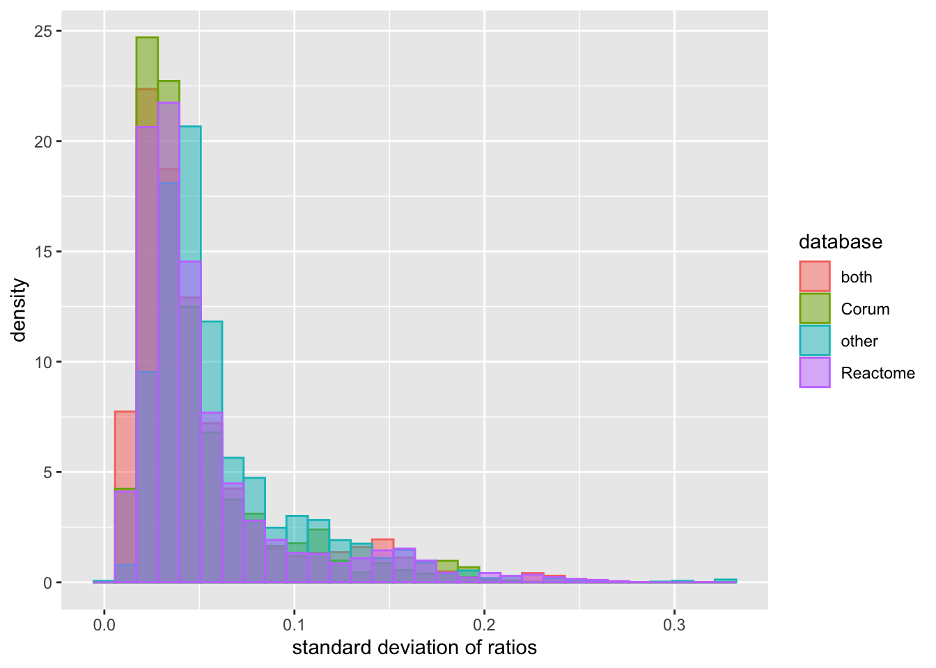 The knowledge of complexes can be obtained from different databases. They may have different reliability. But based on this plot, there’s no significant difference among different databases.
Calculate the ratios of protein pairs not in complexes
Here, I will calculate the ratios of 5000 random protein pairs that are not involved in complexes
n <- nrow(int_pairs)
n <- 5000
allProt <- unique(c(int_pairs$ProtA, int_pairs$ProtB))
randSto <- tibble(ProtA =  rep("",n), ProtB = rep("",n), sdRatio = rep(0,n), inComplex ="no")
i <- 0
while (i <= n-1) {
  ProtA <- sample(allProt, 1)
  ProtB <- sample(allProt, 1)
  pair <- paste0(sort(c(ProtA, ProtB)),collapse = "-")
  if (!pair %in% stoTab$pair) {
    #accept
    i <- i + 1
    randSto[i, 1] <- ProtA
    randSto[i, 2] <- ProtB
    logRatio <- log2(protMat[ProtA,]) - log2(protMat[ProtB,])
    randSto[i, 3] <- sd(logRatio)
  }
}
Compare the standard deviation of expression ratios of pairs in and not in complexes
For all protein pairs
compareTab <- bind_rows(stoTab, randSto)
ggplot(compareTab, aes(x=sdRatio, fill = inComplex, col = inComplex, y=..density..)) +
geom_histogram(position = "identity", alpha = 0.5) +
xlab("standard deviation of ratios")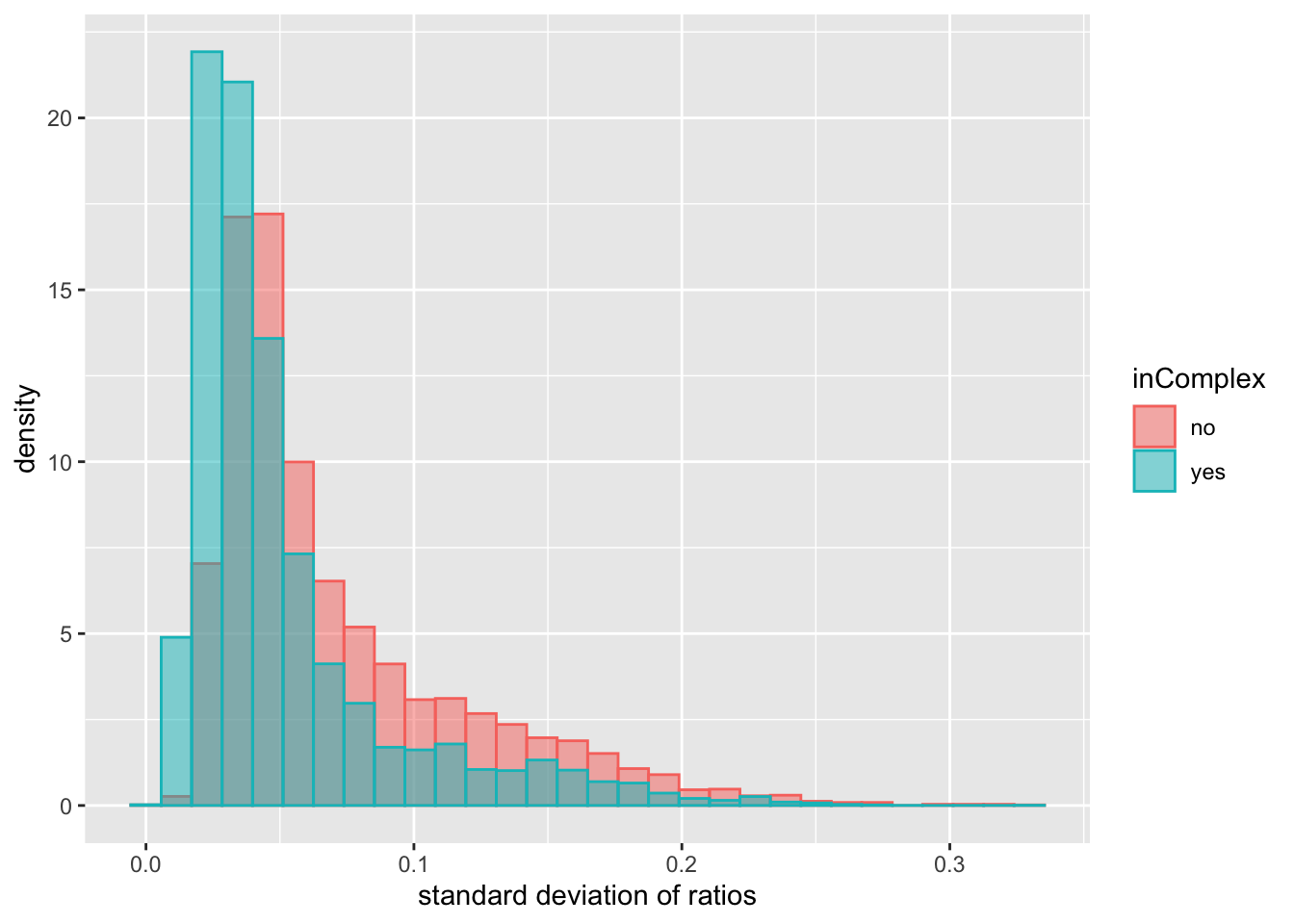 There’s a trend that the protein pairs in complexes have slightly lower standard deviations of expression ratio, indicating more conserved stoichiometry, but the difference is very small.
For all protein pairs with stronger evidence of complex (present in both Corum and Reactome databases)
compareTab <- bind_rows(stoTab, randSto) %>%
filter(database %in% c("both",NA))
ggplot(compareTab, aes(x=sdRatio, fill = inComplex, col = inComplex, y=..density..)) +
geom_histogram(position = "identity", alpha = 0.5)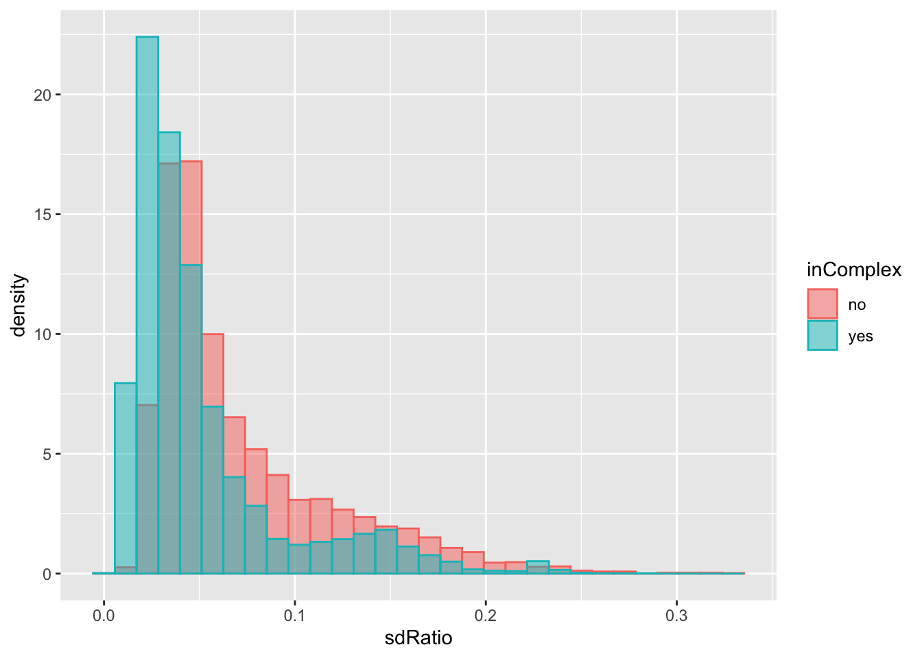 Not too much difference.
Question 2: do protein pairs in complexes really have higher correlation of expression?
I will compare the Pearson correlation coefficients of protein pairs in complexes and not in complexes. A larger coefficient means higher correlation.
Calculate correlations for protein pairs in complexes
corTab <- int_pairs %>% select(ProtA, ProtB, pair, Reactome, Corum, database, inComplex)
protMat <- assays(protSub)[["QRILC"]]
listA <- int_pairs$ProtA
listB <- int_pairs$ProtB
coefList <- rep(NA,nrow(int_pairs))
for (i in seq(length(sdRatio))) {
idA <- listA[i]
idB <- listB[i]
coef <- cor(protMat[idA,], protMat[idB,])
coefList[i] <- coef
}
corTab$coef <- coefList
ggplot(corTab, aes(x=coef, fill = database, col = database, y=..density..)) +
geom_histogram(position = "identity", alpha = 0.5)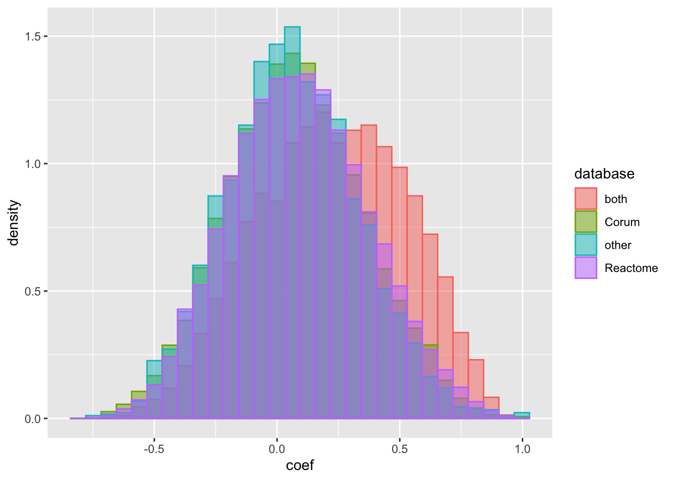 It seems if the protein pairs are annotated as complexes in both Corum and Reactome databases (stronger evidence), they tend to have higher correlation coefficient.
Calculate correlations for random protein pairs not in complexes
n <- nrow(int_pairs)
n <- 5000
allProt <- unique(c(int_pairs$ProtA, int_pairs$ProtB))
randCoef <- tibble(ProtA =  rep("",n), ProtB = rep("",n), coef = rep(0,n), inComplex ="no")
i <- 0
while (i <= n-1) {
  ProtA <- sample(allProt, 1)
  ProtB <- sample(allProt, 1)
  pair <- paste0(sort(c(ProtA, ProtB)),collapse = "-")
  if (!pair %in% corTab$pair) {
    #accept
    i <- i + 1
    randCoef[i, 1] <- ProtA
    randCoef[i, 2] <- ProtB
    coef <- cor(protMat[ProtA,], protMat[ProtB,])
    randCoef[i, 3] <- coef
  }
}
Compare the correlation coefficients of pairs in and not in complexes
For all protein pairs
compareTab <- bind_rows(corTab, randCoef)
ggplot(compareTab, aes(x=coef, fill = inComplex, col = inComplex, y=..density..)) +
geom_histogram(position = "identity", alpha = 0.5)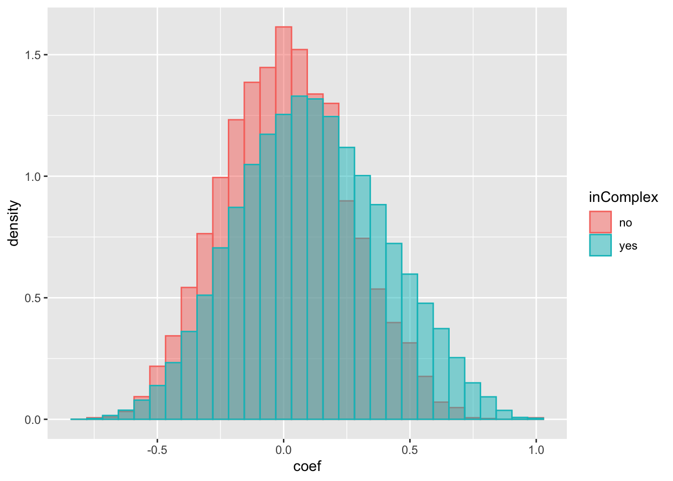 There’s indeed a trend that protein pairs in complex have higher coefficient than protein pairs that not in complexes.
For all protein pairs with stronger evidence of complex (present in both Corum and Reactome databases)
Compare (only from both)
compareTab <- bind_rows(corTab, randCoef) %>%
filter(database %in% c("both",NA))
ggplot(compareTab, aes(x=coef, fill = inComplex, col = inComplex, y=..density..)) +
geom_histogram(position = "identity", alpha = 0.5)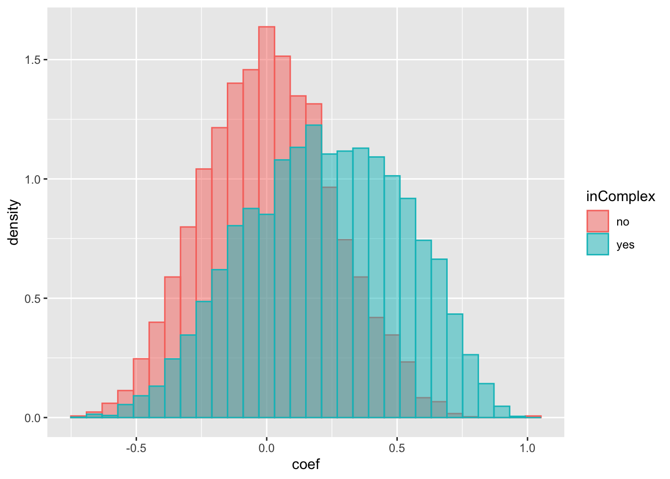 The difference is stronger if I only include proteins with stronger evidence of forming complexes.
However, the correlations observed for protein abundance can also be due to the correlation in RNA expression, not neccessary due to complex formation. I will also test if the RNA expression of protein pairs shows this trend
Correlations on RNA expression level
Correlations of RNA expression levels of proteins in complexs
corTab.rna <- int_pairs %>% select(ProtA, ProtB, pair, Reactome, Corum, database, inComplex)
protMat <- assay(ddsSub.vst)
rownames(protMat) <- rowData(ddsSub.vst)$uniprotID
listA <- int_pairs$ProtA
listB <- int_pairs$ProtB
coefList <- rep(NA,nrow(int_pairs))
for (i in seq(length(coefList))) {
idA <- listA[i]
idB <- listB[i]
coef <- cor(protMat[idA,], protMat[idB,])
coefList[i] <- coef
}
corTab.rna$coef <- coefList
ggplot(corTab.rna, aes(x=coef, fill = database, col = database, y=..density..)) +
geom_histogram(position = "identity", alpha = 0.5)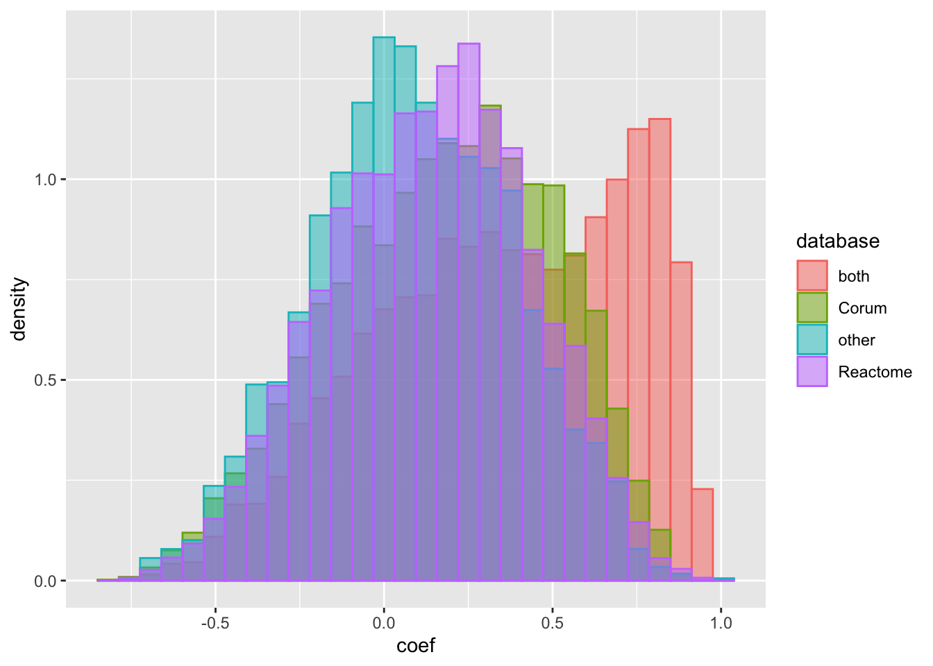 It seems that the RNA expressions of proteins in complex also have higher correlation. The trend is stronger for proteins with stronger evidences of being in complexes.
Correlations of RNA expression levels of random protein pairs not in complexes
n <- nrow(int_pairs)
n <- 5000
allProt <- unique(c(int_pairs$ProtA, int_pairs$ProtB))
randCoef.rna <- tibble(ProtA =  rep("",n), ProtB = rep("",n), coef = rep(0,n), inComplex ="no")
i <- 0
while (i <= n-1) {
  ProtA <- sample(allProt, 1)
  ProtB <- sample(allProt, 1)
  pair <- paste0(sort(c(ProtA, ProtB)),collapse = "-")
  if (!pair %in% corTab$pair) {
    #accept
    i <- i + 1
    randCoef.rna[i, 1] <- ProtA
    randCoef.rna[i, 2] <- ProtB
    coef <- cor(protMat[ProtA,], protMat[ProtB,])
    randCoef.rna[i, 3] <- coef
  }
}
Compare the correlation coefficients of pairs in and not in complexes
For all pairs
compareTab <- bind_rows(corTab.rna, randCoef.rna)
ggplot(compareTab, aes(x=coef, fill = inComplex, col = inComplex, y=..density..)) +
  geom_histogram(position = "identity", alpha = 0.5)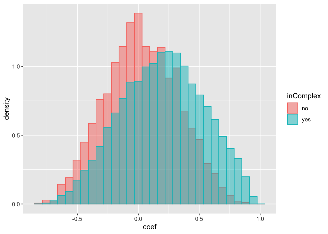
For all pairs with stronger evidence of complex (present in both Corum and Reactome databases)
compareTab <- bind_rows(corTab.rna, randCoef.rna) %>%
filter(database %in% c("both",NA))
ggplot(compareTab, aes(x=coef, fill = inComplex, col = inComplex, y=..density..)) +
geom_histogram(position = "identity", alpha = 0.5)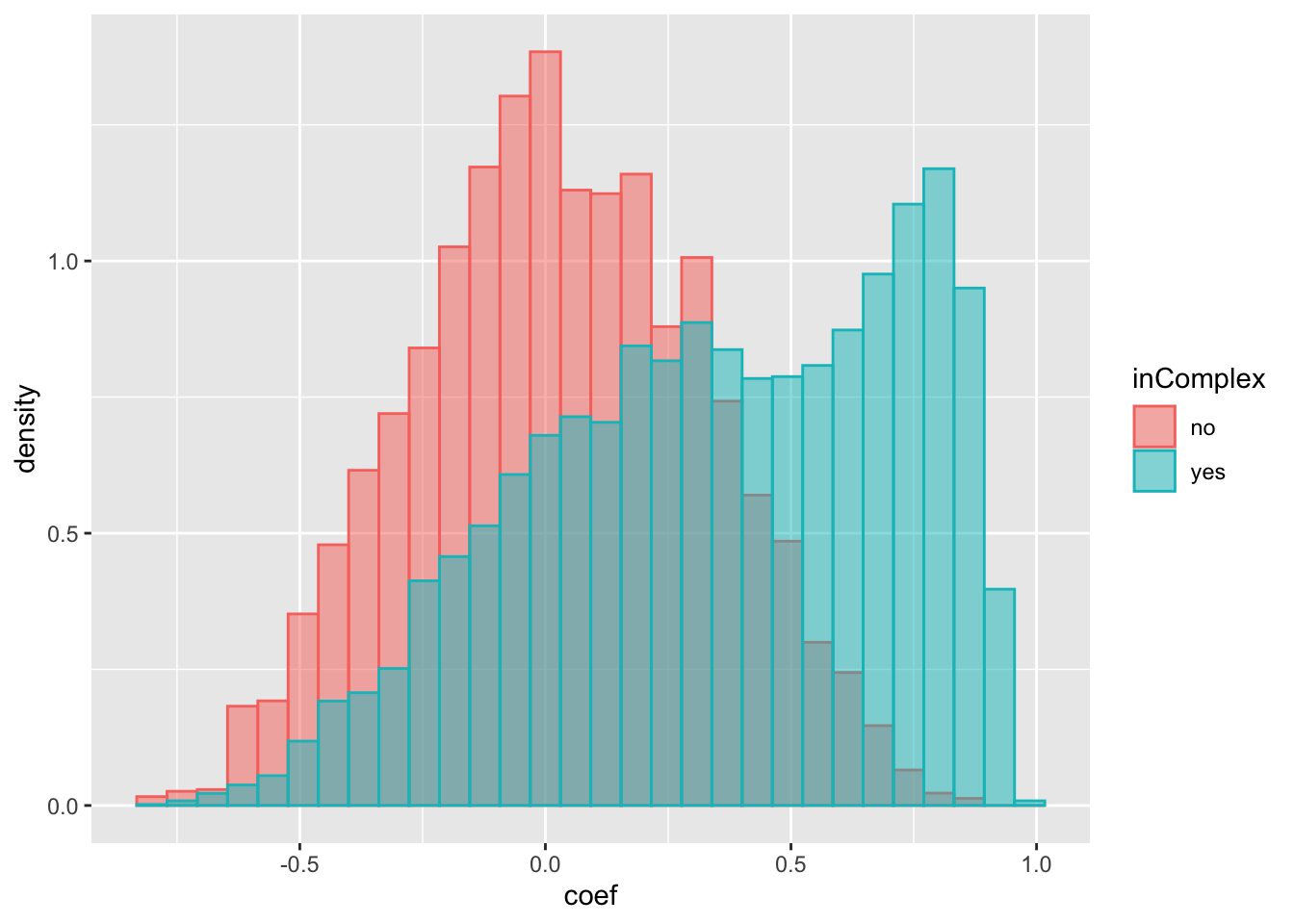 The trend is almost the same as for protein expressions. Which means the higher correlation observed for protein pairs in complexes can simply because their RNA expressions are correlated. Not necessarily because of the complex formation.
Compare the correlation coefficients of protein expression and RNA expression for protein pairs that are annotated as in complexes
compareTab <- bind_rows(mutate(corTab, set = "Protein"), mutate(corTab.rna, set = "RNA"))
ggplot(compareTab, aes(x=coef, fill = set, col = set, y=..density..)) +
geom_histogram(position = "identity", alpha = 0.5)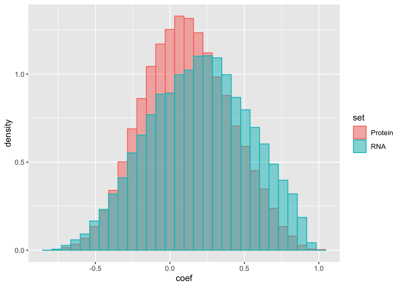 There’s no strong difference. The RNA expressions of protein pairs in complexes even have higher correlations than the corresponding protein expression. This somewaht contradicts previous report that the proteins expressions are more correlations for proteins in complexes than their RNA expressions. However, one explanation is that, if two proteins are annotated as complexes, there’s also a high chance that they are in the same pathway and therefore, their RNAs are also co-expressed.
sessionInfo()R version 3.6.0 (2019-04-26)
Platform: x86_64-apple-darwin15.6.0 (64-bit)
Running under: macOS 10.15.4
Matrix products: default
BLAS: /Library/Frameworks/R.framework/Versions/3.6/Resources/lib/libRblas.0.dylib
LAPACK: /Library/Frameworks/R.framework/Versions/3.6/Resources/lib/libRlapack.dylib
locale:
[1] en_US.UTF-8/en_US.UTF-8/en_US.UTF-8/C/en_US.UTF-8/en_US.UTF-8
attached base packages:
[1] parallel stats4 stats graphics grDevices utils datasets
[8] methods base
other attached packages:
[1] forcats_0.4.0 stringr_1.4.0
[3] dplyr_0.8.5 purrr_0.3.3
[5] readr_1.3.1 tidyr_1.0.0
[7] tibble_3.0.0 ggplot2_3.3.0
[9] tidyverse_1.3.0 DESeq2_1.24.0
[11] SummarizedExperiment_1.14.0 DelayedArray_0.10.0
[13] BiocParallel_1.18.0 matrixStats_0.54.0
[15] Biobase_2.44.0 GenomicRanges_1.36.0
[17] GenomeInfoDb_1.20.0 IRanges_2.18.1
[19] S4Vectors_0.22.0 BiocGenerics_0.30.0
loaded via a namespace (and not attached):
[1] nlme_3.1-140 bitops_1.0-6 fs_1.4.0
[4] lubridate_1.7.4 bit64_0.9-7 httr_1.4.1
[7] RColorBrewer_1.1-2 rprojroot_1.3-2 tools_3.6.0
[10] backports_1.1.4 R6_2.4.0 rpart_4.1-15
[13] Hmisc_4.2-0 DBI_1.0.0 colorspace_1.4-1
[16] nnet_7.3-12 withr_2.1.2 tidyselect_1.0.0
[19] gridExtra_2.3 bit_1.1-14 compiler_3.6.0
[22] git2r_0.26.1 rvest_0.3.5 cli_1.1.0
[25] htmlTable_1.13.1 xml2_1.2.2 labeling_0.3
[28] scales_1.1.0 checkmate_2.0.0 genefilter_1.66.0
[31] digest_0.6.19 foreign_0.8-71 rmarkdown_1.13
[34] XVector_0.24.0 base64enc_0.1-3 pkgconfig_2.0.2
[37] htmltools_0.4.0 dbplyr_1.4.2 readxl_1.3.1
[40] htmlwidgets_1.3 rlang_0.4.5 rstudioapi_0.10
[43] RSQLite_2.1.1 farver_2.0.3 generics_0.0.2
[46] jsonlite_1.6 acepack_1.4.1 RCurl_1.95-4.12
[49] magrittr_1.5 GenomeInfoDbData_1.2.1 Formula_1.2-3
[52] Matrix_1.2-17 Rcpp_1.0.1 munsell_0.5.0
[55] lifecycle_0.2.0 stringi_1.4.3 yaml_2.2.0
[58] zlibbioc_1.30.0 grid_3.6.0 blob_1.1.1
[61] promises_1.0.1 crayon_1.3.4 lattice_0.20-38
[64] haven_2.2.0 splines_3.6.0 annotate_1.62.0
[67] hms_0.5.2 locfit_1.5-9.1 knitr_1.23
[70] pillar_1.4.3 geneplotter_1.62.0 reprex_0.3.0
[73] XML_3.98-1.20 glue_1.3.2 evaluate_0.14
[76] latticeExtra_0.6-28 modelr_0.1.5 data.table_1.12.2
[79] vctrs_0.2.4 httpuv_1.5.1 cellranger_1.1.0
[82] gtable_0.3.0 assertthat_0.2.1 xfun_0.8
[85] xtable_1.8-4 broom_0.5.2 later_0.8.0
[88] survival_2.44-1.1 AnnotationDbi_1.46.0 memoise_1.1.0
[91] workflowr_1.6.0 cluster_2.1.0 ellipsis_0.2.0