Protein complex regulation analysis of trisomy12
Junyan Lu
2020-05-22
Last updated: 2020-06-02
Checks: 5 2
Knit directory: Proteomics/analysis/
This reproducible R Markdown analysis was created with workflowr (version 1.6.0). The Checks tab describes the reproducibility checks that were applied when the results were created. The Past versions tab lists the development history.
The R Markdown is untracked by Git. To know which version of the R Markdown file created these results, you’ll want to first commit it to the Git repo. If you’re still working on the analysis, you can ignore this warning. When you’re finished, you can run wflow_publish to commit the R Markdown file and build the HTML.
Great job! The global environment was empty. Objects defined in the global environment can affect the analysis in your R Markdown file in unknown ways. For reproduciblity it’s best to always run the code in an empty environment.
The command set.seed(20200227) was run prior to running the code in the R Markdown file. Setting a seed ensures that any results that rely on randomness, e.g. subsampling or permutations, are reproducible.
Great job! Recording the operating system, R version, and package versions is critical for reproducibility.
- unnamed-chunk-13
- unnamed-chunk-15
- unnamed-chunk-16
- unnamed-chunk-20
- unnamed-chunk-4
- unnamed-chunk-5
- unnamed-chunk-6
- unnamed-chunk-8
To ensure reproducibility of the results, delete the cache directory complexAnalysis_trisomy12_cache and re-run the analysis. To have workflowr automatically delete the cache directory prior to building the file, set delete_cache = TRUE when running wflow_build() or wflow_publish().
Great job! Using relative paths to the files within your workflowr project makes it easier to run your code on other machines.
Great! You are using Git for version control. Tracking code development and connecting the code version to the results is critical for reproducibility. The version displayed above was the version of the Git repository at the time these results were generated.
Note that you need to be careful to ensure that all relevant files for the analysis have been committed to Git prior to generating the results (you can use wflow_publish or wflow_git_commit). workflowr only checks the R Markdown file, but you know if there are other scripts or data files that it depends on. Below is the status of the Git repository when the results were generated:
Ignored files:
    Ignored:    .DS_Store
    Ignored:    .Rhistory
    Ignored:    .Rproj.user/
    Ignored:    analysis/.DS_Store
    Ignored:    analysis/.Rhistory
    Ignored:    analysis/complexAnalysis_IGHV_cache/
    Ignored:    analysis/complexAnalysis_trisomy12_alteredPQR_cache/
    Ignored:    analysis/complexAnalysis_trisomy12_cache/
    Ignored:    analysis/correlateCLLPD_cache/
    Ignored:    code/.Rhistory
    Ignored:    data/.DS_Store
    Ignored:    output/.DS_Store

Untracked files:
    Untracked:  analysis/CNVanalysis_11q.Rmd
    Untracked:  analysis/CNVanalysis_trisomy12.Rmd
    Untracked:  analysis/CNVanalysis_trisomy19.Rmd
    Untracked:  analysis/analysisSplicing.Rmd
    Untracked:  analysis/analysisTrisomy19.Rmd
    Untracked:  analysis/annotateCNV.Rmd
    Untracked:  analysis/complexAnalysis_IGHV.Rmd
    Untracked:  analysis/complexAnalysis_trisomy12.Rmd
    Untracked:  analysis/correlateGenomic_PC12adjusted.Rmd
    Untracked:  analysis/correlateGenomic_noBlock.Rmd
    Untracked:  analysis/correlateGenomic_noBlock_MCLL.Rmd
    Untracked:  analysis/correlateGenomic_noBlock_UCLL.Rmd
    Untracked:  analysis/default.css
    Untracked:  analysis/del11q.pdf
    Untracked:  analysis/del11q_norm.pdf
    Untracked:  analysis/peptideValidate.Rmd
    Untracked:  analysis/plotExpressionCNV.Rmd
    Untracked:  analysis/processPeptides_LUMOS.Rmd
    Untracked:  analysis/style.css
    Untracked:  analysis/trisomy12.pdf
    Untracked:  analysis/trisomy12_AFcor.Rmd
    Untracked:  analysis/trisomy12_norm.pdf
    Untracked:  code/AlteredPQR.R
    Untracked:  code/utils.R
    Untracked:  data/190909_CLL_prot_abund_med_norm.tsv
    Untracked:  data/190909_CLL_prot_abund_no_norm.tsv
    Untracked:  data/20190423_Proteom_submitted_samples_bereinigt.xlsx
    Untracked:  data/20191025_Proteom_submitted_samples_final.xlsx
    Untracked:  data/LUMOS/
    Untracked:  data/LUMOS_peptides/
    Untracked:  data/LUMOS_protAnnotation.csv
    Untracked:  data/LUMOS_protAnnotation_fix.csv
    Untracked:  data/SampleAnnotation_cleaned.xlsx
    Untracked:  data/example_proteomics_data
    Untracked:  data/facTab_IC50atLeast3New.RData
    Untracked:  data/gmts/
    Untracked:  data/mapEnsemble.txt
    Untracked:  data/mapSymbol.txt
    Untracked:  data/proteins_in_complexes
    Untracked:  data/pyprophet_export_aligned.csv
    Untracked:  data/timsTOF_protAnnotation.csv
    Untracked:  output/LUMOS_processed.RData
    Untracked:  output/cnv_plots.zip
    Untracked:  output/cnv_plots/
    Untracked:  output/cnv_plots_norm.zip
    Untracked:  output/dxdCLL.RData
    Untracked:  output/exprCNV.RData
    Untracked:  output/pepCLL_lumos.RData
    Untracked:  output/pepTab_lumos.RData
    Untracked:  output/plotCNV_allChr11_diff.pdf
    Untracked:  output/plotCNV_del11q_sum.pdf
    Untracked:  output/proteomic_LUMOS_20200227.RData
    Untracked:  output/proteomic_LUMOS_20200320.RData
    Untracked:  output/proteomic_LUMOS_20200430.RData
    Untracked:  output/proteomic_timsTOF_20200227.RData
    Untracked:  output/splicingResults.RData
    Untracked:  output/timsTOF_processed.RData
    Untracked:  plotCNV_del11q_diff.pdf

Unstaged changes:
    Modified:   analysis/_site.yml
    Modified:   analysis/analysisSF3B1.Rmd
    Modified:   analysis/compareProteomicsRNAseq.Rmd
    Modified:   analysis/correlateCLLPD.Rmd
    Modified:   analysis/correlateGenomic.Rmd
    Deleted:    analysis/correlateGenomic_removePC.Rmd
    Modified:   analysis/correlateMIR.Rmd
    Modified:   analysis/correlateMethylationCluster.Rmd
    Modified:   analysis/index.Rmd
    Modified:   analysis/predictOutcome.Rmd
    Modified:   analysis/processProteomics_LUMOS.Rmd
    Modified:   analysis/qualityControl_LUMOS.Rmd
Note that any generated files, e.g. HTML, png, CSS, etc., are not included in this status report because it is ok for generated content to have uncommitted changes.
There are no past versions. Publish this analysis with wflow_publish() to start tracking its development.
Load libraries and dataset
library(SummarizedExperiment)
library(tidygraph)
library(DGCA)
library(proDA)
library(DESeq2)
library(cowplot)
library(igraph)
library(ggraph)
library(tidyverse)
Prepare datasets
Using datasets
load("../output/proteomic_LUMOS_20200430.RData")
load("../../var/patmeta_200522.RData")
load("../../var/ddsrna_180717.RData")
Using the protein complex information from database CORUM
int_pairs = read.table ("../data/proteins_in_complexes", sep = "\t", stringsAsFactors = FALSE, header = T)I use the comparison of whether the patients have trisomy12 (a gain of extra copy of chromosome 12). The patients without trisomy12 are defined the as the reference.
The analysis goal is to see whether the gene dosage effect from the extra copy of trisomy12 affect protein complexes landscape in patient samples with trisomy12
Differential protein expression analysis
Detect protein abundance changes related to trisomy12
exprMat <- assays(protCLL)[["count"]]
designMat <- data.frame(row.names  = colnames(protCLL), IGHV = protCLL$IGHV.status, trisomy12 = protCLL$trisomy12)
fit <- proDA(exprMat, design = ~ .,
             col_data = designMat)
corRes <- test_diff(fit, "trisomy121") %>%
    dplyr::rename(id = name, logFC = diff, t=t_statistic,
                  P.Value = pval, adj.P.Val = adj_pval) %>%
    mutate(name = rowData(protCLL[id,])$hgnc_symbol) %>%
    select(name, id, logFC, t, P.Value, adj.P.Val) %>%
    arrange(P.Value) %>% as_tibble()

corRes.sig <- filter(corRes, adj.P.Val <0.05) %>%
  mutate(direction = ifelse(t>0, "Up","Down"))
Detect differential complex formations based on the algorithm from Marija Buljan
The hypothesis of the algorithm is that the ratio (stoichiometry) of two proteins in a complex in the reference set follows a certain distribution. If the distribution of the ratios in the test set deviates from the distribution of the reference set, this indicates a change of stoichiometry in the test set and therefore a potential change of the complex formations.
One of the caveats of this algorithm is that it relies on outlier detection and therefore need hard cut-off values to define outliers and the fraction of outliers in the test set. Another caveat is that a simple up-regulation or down-regulation in the pair will also change the ratio. But this change of ratio may not really result from complex changes.
Run AlteredPRQ algorithm to detect protein complex ratio complex changes
source ("../code/AlteredPQR.R")
quant_data_all = assays(protCLL)[["QRILC"]]
cols_with_reference_data = seq(ncol(protCLL))[protCLL$trisomy12 %in% 0]
RepresentativePairs = Altered_PQR(modif_z_score_threshold = 3.0, fraction_of_samples_threshold = 0.3)
[1] "Running"
[1] "..."
[1] "..."
[1] "Top 0.1, 1 and 5% upper and lower z-score values are: 8.26742846535531 3.93569392733038 2.19885719576535 and -6.27632295669363 -3.42621202641534 -1.92712652454253."
[1] "Top 1% of the absolute values for the modified z-scores is 4.55241553106446."Re-format output
protRes.pqr <- lapply(RepresentativePairs, function(x) x) %>% bind_cols() %>%
  separate(Protein_pair, into = c("idA","idB"),"-") %>%
  mutate(protA = rowData(protCLL[idA,])$hgnc_symbol,
         protB = rowData(protCLL[idB,])$hgnc_symbol,
         chrA = rowData(protCLL[idA,])$chromosome_name,
         chrB = rowData(protCLL[idB,])$chromosome_name) %>%
  mutate(withChr12 = ifelse(chrA %in% "12" | chrB%in% "12", "yes", "no"))%>% mutate(idx = seq(nrow(.))) %>%
  mutate(pair=map2_chr(idA, idB, ~paste0(sort(c(.x,.y)), collapse = "-")))
Run the same algorithm on RNA expression data
dds$trisomy12 <- patMeta[match(dds$PatID,patMeta$Patient.ID),]$trisomy12
rowData(dds)$uniprotID <- rownames(protCLL)[match(rownames(dds), rowData(protCLL)$ensembl_gene_id)]
ddsSub <- dds[!is.na(rowData(dds)$uniprotID), dds$PatID %in% colnames(protCLL)]
rownames(ddsSub) <- rowData(ddsSub)$uniprotID
ddsSub.vst <- varianceStabilizingTransformation(ddsSub)
source ("../code/AlteredPQR.R")
quant_data_all = assay(ddsSub.vst)
cols_with_reference_data = seq(ncol(ddsSub.vst))[ddsSub.vst$trisomy12 %in% 0]
RepresentativePairs = Altered_PQR(modif_z_score_threshold = 3.0, fraction_of_samples_threshold = 0.3)[1] "Running"
[1] "..."
[1] "..."
[1] "Top 0.1, 1 and 5% upper and lower z-score values are: 9.02665546130853 3.95530891659894 2.44967137434484 and -6.48456606482675 -3.77874942568752 -2.3012824895991."
[1] "Top 1% of the absolute values for the modified z-scores is 4.61537110973003."rnaRes.pqr <- lapply(RepresentativePairs, function(x) x) %>% bind_cols() %>%
separate(Protein_pair, into = c("idA","idB"),"-") %>%
dplyr::rename(rnaChange = Change, rnaScore= Score) %>%
mutate(pair=map2_chr(idA, idB, ~paste0(sort(c(.x,.y)), collapse = "-"))) %>%
select(pair, rnaScore, rnaChange)Combine protein and RNA result
comRes.pqr <- left_join(protRes.pqr, rnaRes.pqr, by ="pair") %>%
  mutate(explainedByRNA = ifelse(is.na(rnaChange), "no",
                                 ifelse(Change == rnaChange, "yes", "no")))
Exploring results
Whether protein pairs involve genes on Chr12 have higher score?
ggplot(comRes.pqr, aes(x=Score, fill = withChr12, col = withChr12)) + geom_histogram(alpha=0.5, position = "identity") + theme_bw()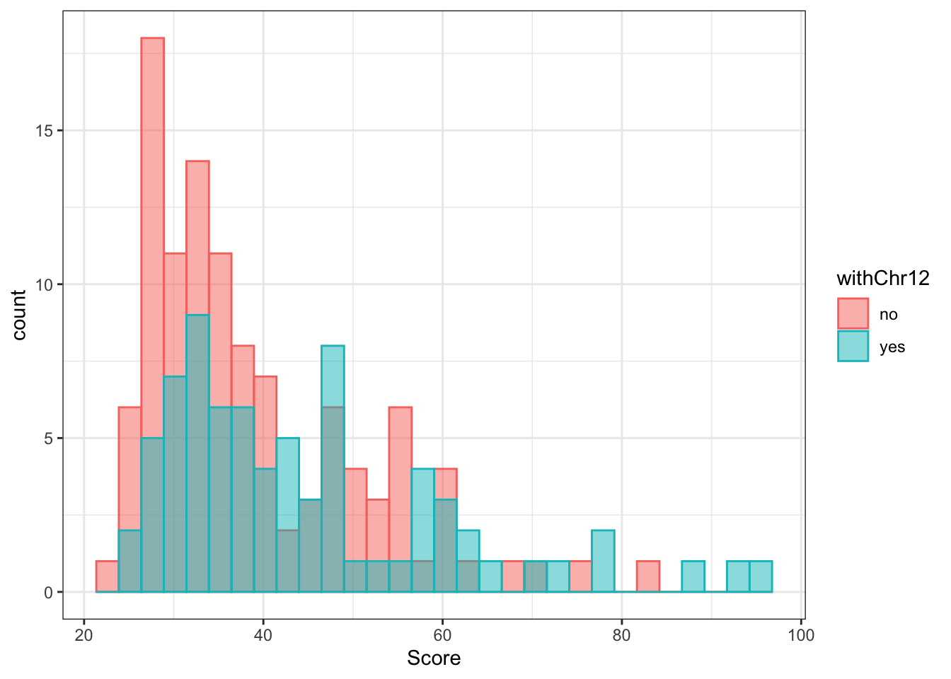 Not really, but there are some chr12 pairs have extremely high score.
How many of those changes can be explained at RNA level
table(comRes.pqr$explainedByRNA)
 no yes
183   2
Only 2
List of detected pairs
comRes.pqr %>% select(protA, protB, Score, Change, chrA, chrB, withChr12, explainedByRNA) %>%
  mutate(Score = format(Score, digits = 1)) %>%
  DT::datatable()
Visualization using network plot
Only pairs involving genes on chr12 are used for now Build network
comRes.filt <- filter(comRes.pqr, Score > 0, withChr12 == "yes")

#get node list
allNodes <- union(comRes.filt$protA, comRes.filt$protB)

nodeList <- data.frame(id = seq(length(allNodes))-1, name = allNodes, stringsAsFactors = FALSE) %>%
  mutate(onChr12 = ifelse(rowData(protCLL[match(name, rowData(protCLL)$hgnc_symbol),])$chromosome_name %in% "12",
                          "chr12","otherChr")) %>%
  mutate(group = corRes.sig[match(name, corRes.sig$name),]$direction) %>%
  mutate(group = ifelse(is.na(group),"ns",group))

#get edge list
edgeList <- select(comRes.filt, protA, protB, Change, explainedByRNA) %>%
  dplyr::rename(Source = protA, Target = protB) %>%
  mutate(Source = nodeList[match(Source,nodeList$name),]$id,
         Target = nodeList[match(Target, nodeList$name),]$id) %>%
  data.frame(stringsAsFactors = FALSE)

net <- graph_from_data_frame(vertices = nodeList, d=edgeList, directed = FALSE)
Visualize using ggraph
tidyNet <- as_tbl_graph(net)
ggraph(tidyNet) + geom_edge_link(aes(color = Change, edge_linetype = explainedByRNA), width=1) +
geom_node_point(aes(color =group, shape = onChr12), size=4) +
geom_node_text(aes(label = name), repel = TRUE) +
scale_color_manual(values = c(Up = "pink",Down = "lightblue", ns="grey"))+
theme_graph() 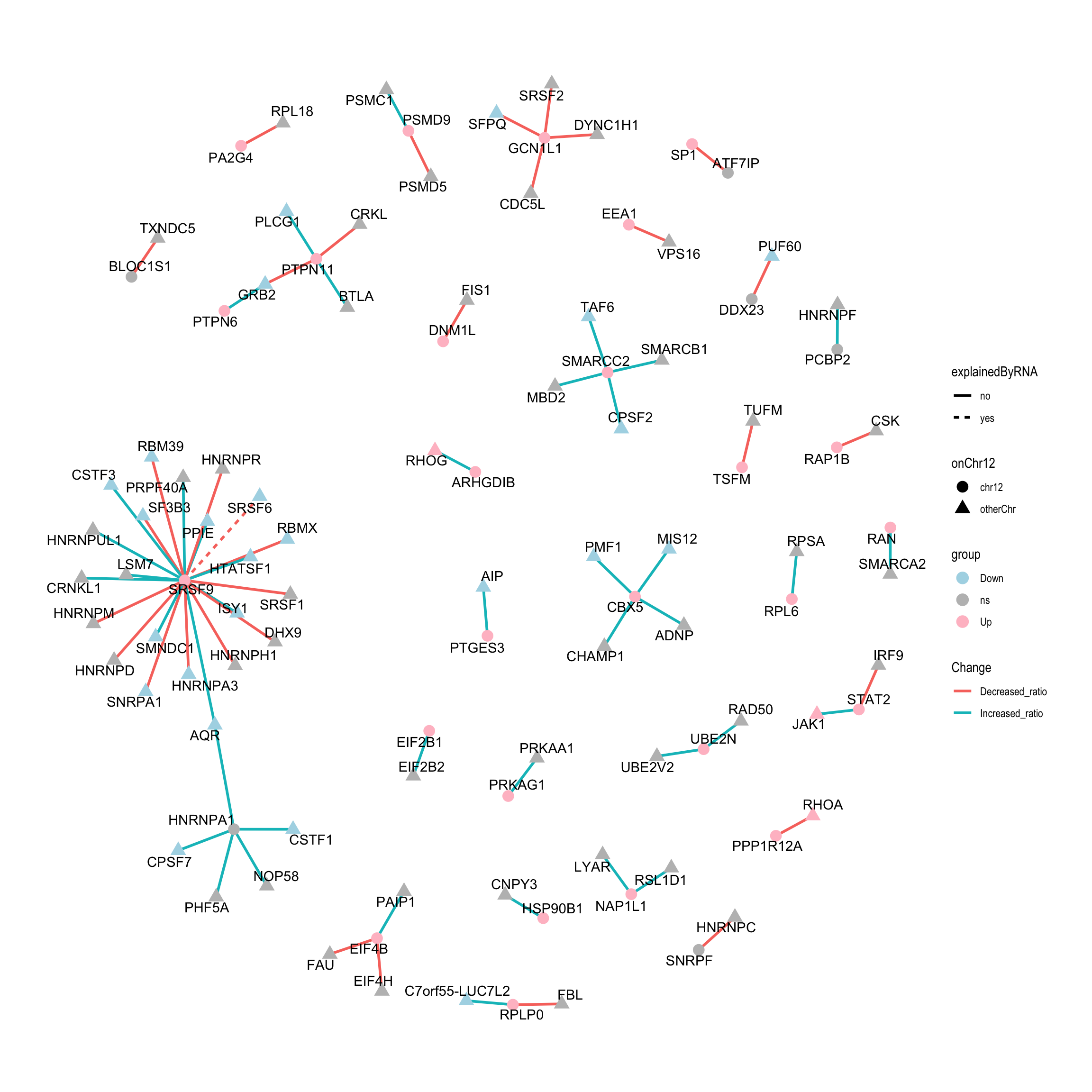 In this plot, proteins on Chr12 are shown as solid circles and others are shown as triangles. The proteins up-regulated in trisomy12 samples are colored by red, down-regulated proteins are colored by cyan and the proteins with no significant changes are colored by grey. The color of the edges indication the whether the ratio of two proteins in pairs are increased or decreased in the reference group. But I don’t think this value has real biological meaning. It depends which protein is placed as the first one when calculating the ratio.
Inspecting some interesting pairs
plotPair <- function(comRes, protList, protCLL, gene) {
  pairList <- filter(comRes, protA %in% protList | protB %in% protList)
  plotList <- lapply(seq(nrow(pairList)), function(i) {
    idA <- pairList[i,]$idA
    idB <- pairList[i,]$idB
    protA <- pairList[i,]$protA
    protB  <- pairList[i,]$protB
    idPair <- c(idA, idB)
    protPair <- c(protA, protB)
    ord <- order(protPair)
    idPair <- idPair[ord]
    protPair <- protPair[ord]
    plotTab <- assays(protCLL)[["count"]][idPair,] %>%
      t() %>% data.frame()
    colnames(plotTab) <- protPair
    plotTab$logRatio <- log2(plotTab[,1]) - log2(plotTab[,2])
    plotTab <- rownames_to_column(plotTab,"patID") %>%
      mutate(status = factor(protCLL[,patID][[gene]])) %>%
      filter(!is.na(logRatio))
    histP <- ggplot(plotTab, aes(x=logRatio, fill = status, col = status)) +
      geom_histogram(position = "identity", alpha=0.5) +
      ggtitle(sprintf("Stoichiometry: %s ~ %s",protPair[1], protPair[2]))
    corP <- ggplot(plotTab, aes_string(x=protPair[1], y=protPair[2], col="status")) +
      geom_point() + geom_smooth(formula = y~x, method = "lm") +
      scale_color_discrete(name = gene)
    plot_grid(histP, corP)
  })
  return(plotList)
}
plotPair.rna <- function(comRes, protList, ddsSub.vst, gene) {
pairList <- filter(comRes, protA %in% protList | protB %in% protList)
plotList <- lapply(seq(nrow(pairList)), function(i) {
idA <- pairList[i,]$idA
idB <- pairList[i,]$idB
protA <- pairList[i,]$protA
protB <- pairList[i,]$protB
idPair <- c(idA, idB)
protPair <- c(protA, protB)
ord <- order(protPair)
idPair <- idPair[ord]
protPair <- protPair[ord]
plotTab <- assay(ddsSub.vst)[idPair,] %>%
t() %>% data.frame()
colnames(plotTab) <- protPair
plotTab$logRatio <- log2(plotTab[,1]) - log2(plotTab[,2])
plotTab <- rownames_to_column(plotTab,"patID") %>%
mutate(status = factor(ddsSub.vst[,patID][[gene]])) %>%
filter(!is.na(logRatio))
histP <- ggplot(plotTab, aes(x=logRatio, fill = status, col = status)) +
geom_histogram(position = "identity", alpha=0.5) +
ggtitle(sprintf("Stoichiometry: %s ~ %s",protPair[1], protPair[2]))
corP <- ggplot(plotTab, aes_string(x=protPair[1], y=protPair[2], col="status")) +
geom_point() + geom_smooth(formula = y~x, method = "lm") +
scale_color_discrete(name = gene)
plot_grid(histP, corP)
})
return(plotList)
}Pairs involving PTPN6 and PTPN11
protList <- c("PTPN6","PTPN11")
plotPair(comRes.pqr, protList, protCLL, "trisomy12")
[[1]]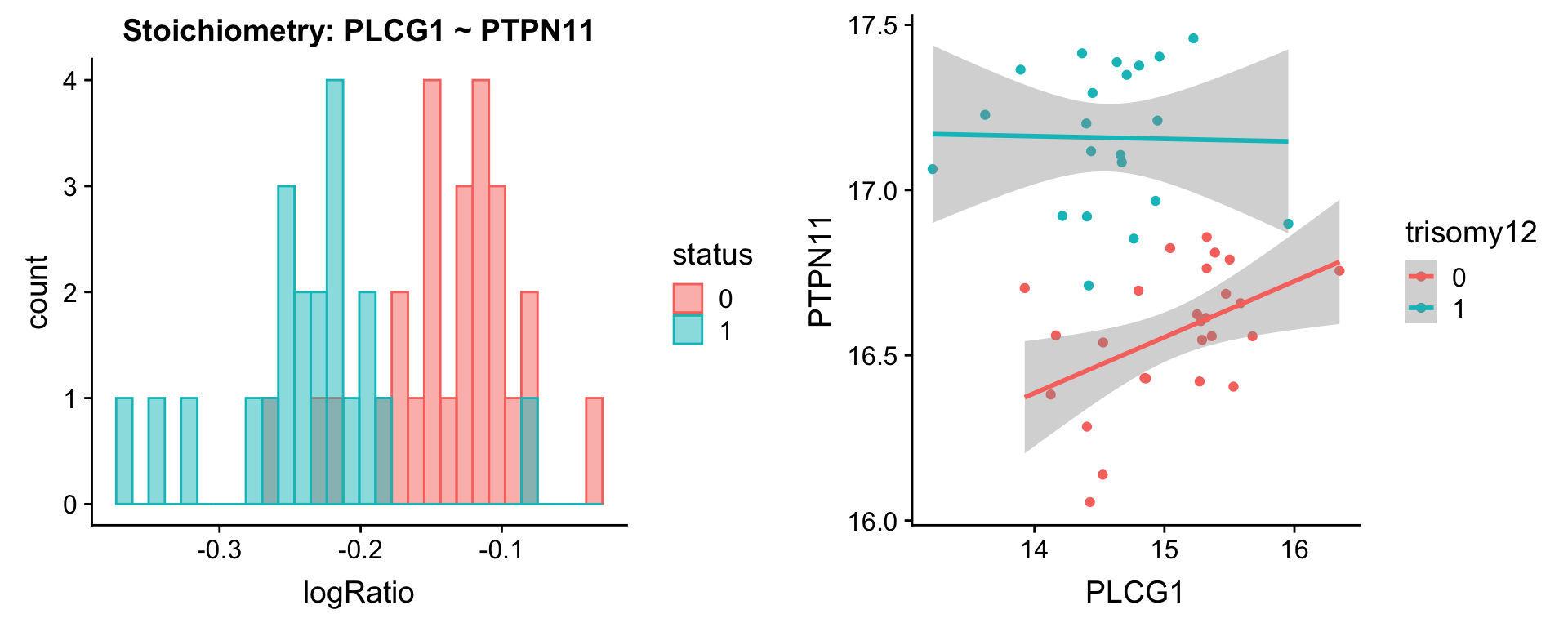
[[2]]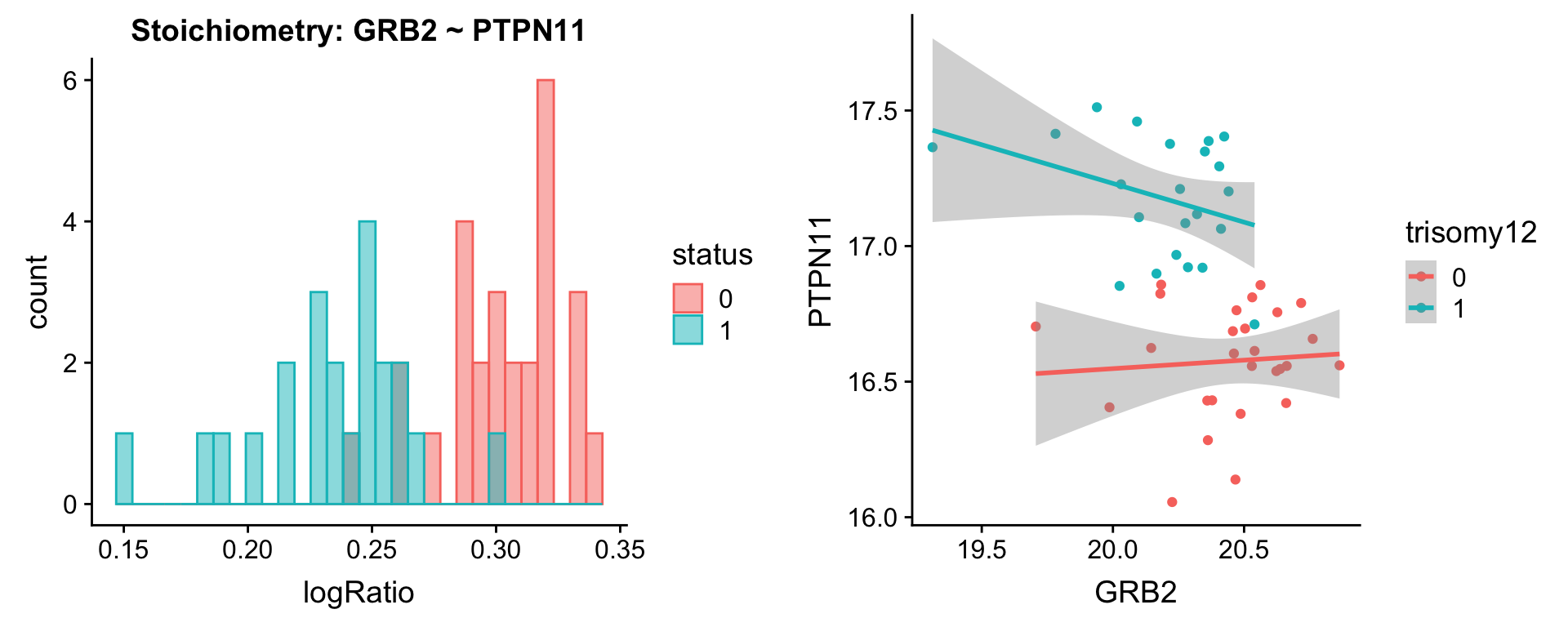
[[3]]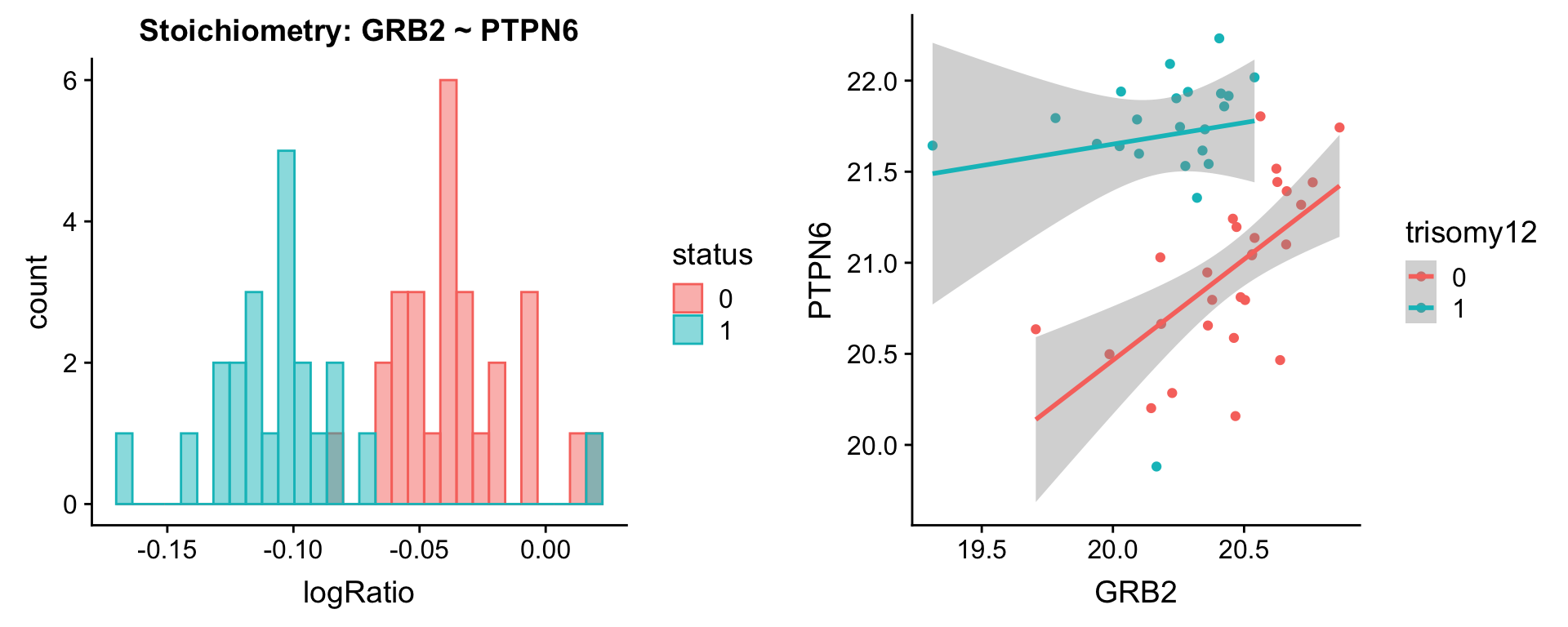
[[4]]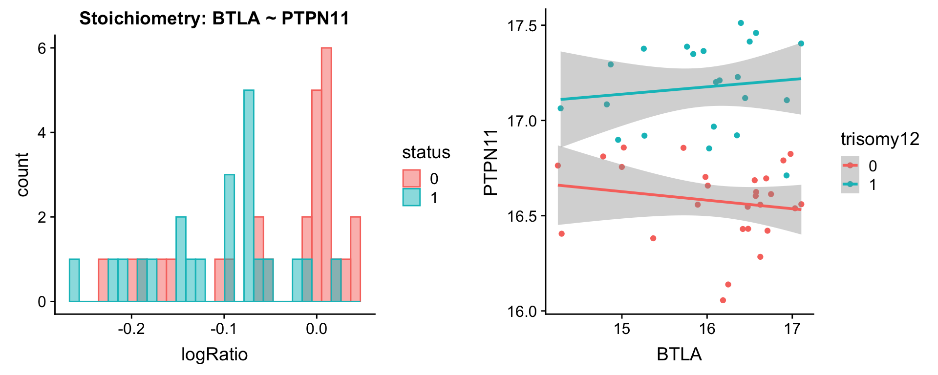
[[5]]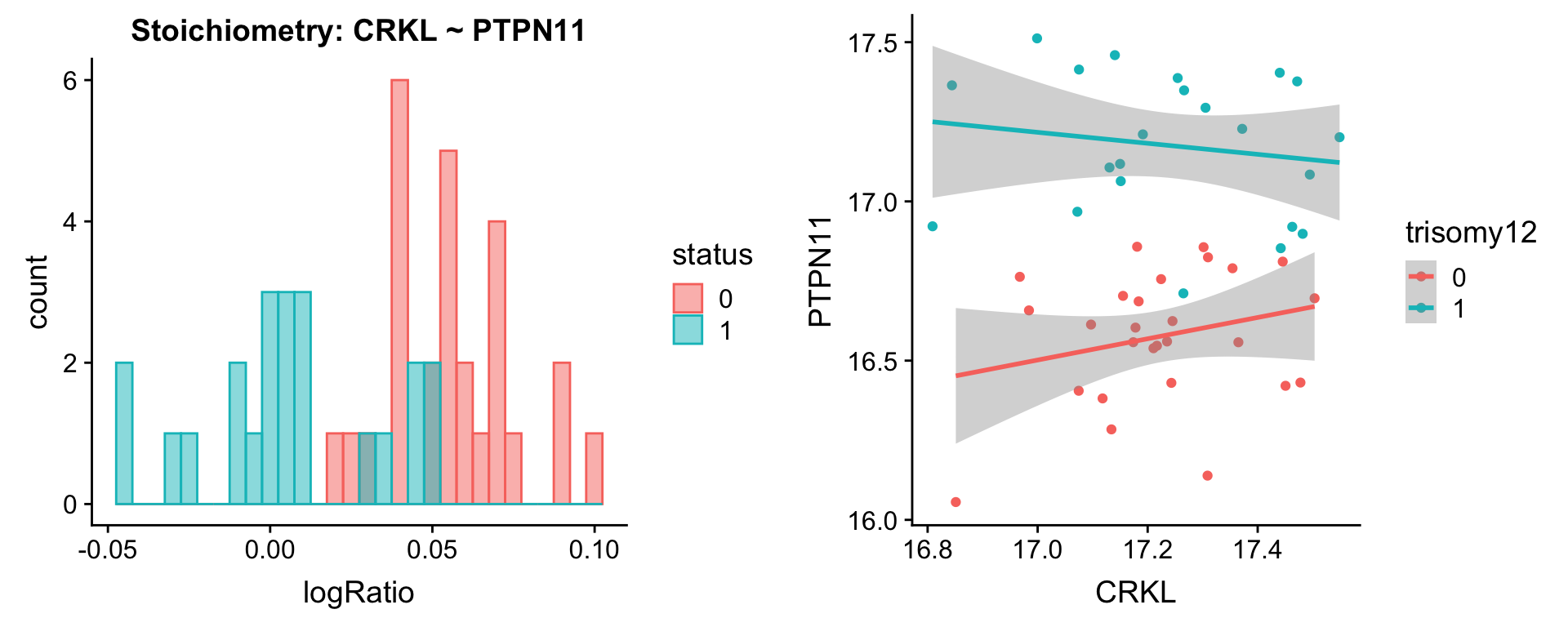
Pairs involving STAT2
protList <- c("STAT2")
plotPair(comRes.pqr, protList, protCLL, "trisomy12")
[[1]]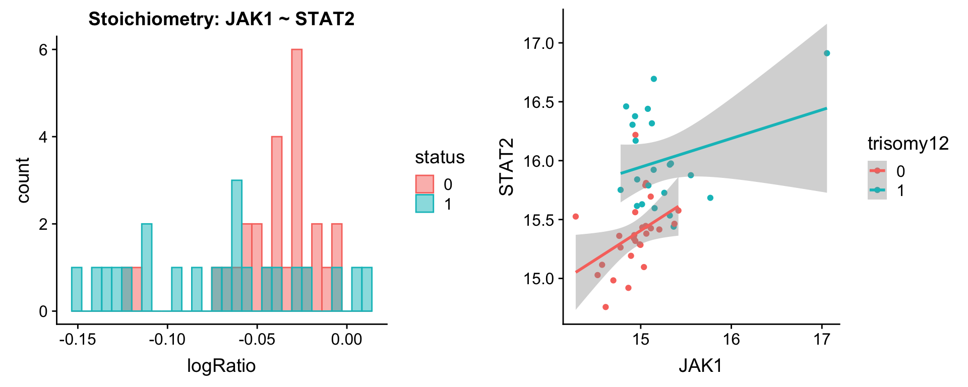
[[2]]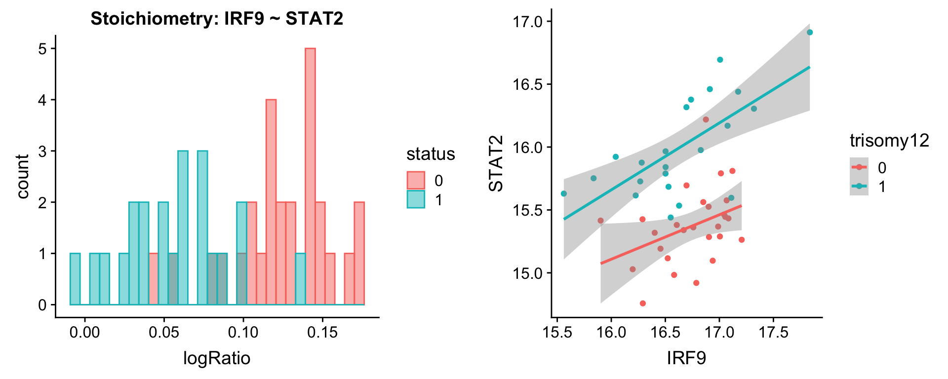
Check those pairs at RNA level
Pairs involving PTPN6 and PTPN11
protList <- c("PTPN6","PTPN11")
plotPair.rna(comRes.pqr, protList, ddsSub.vst, "trisomy12")
[[1]]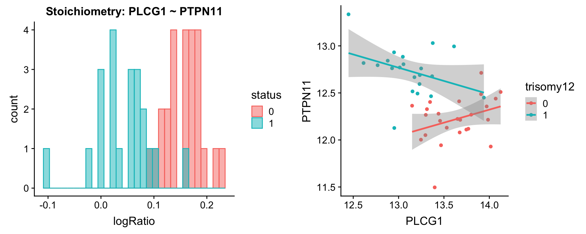
[[2]]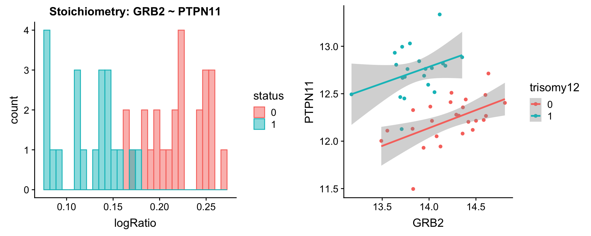
[[3]]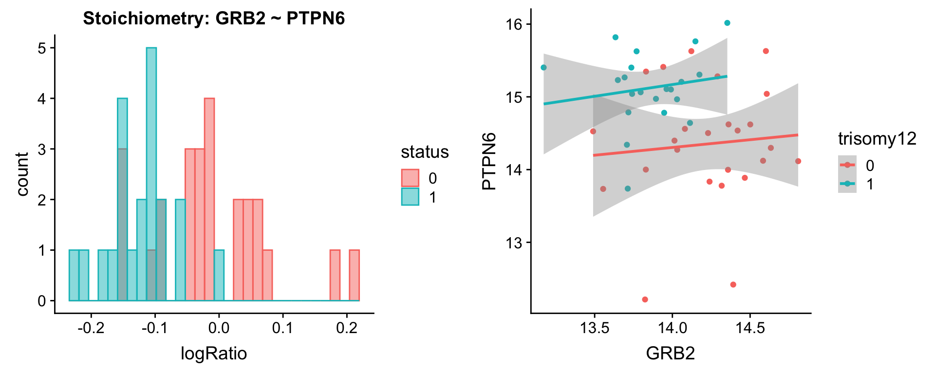
[[4]]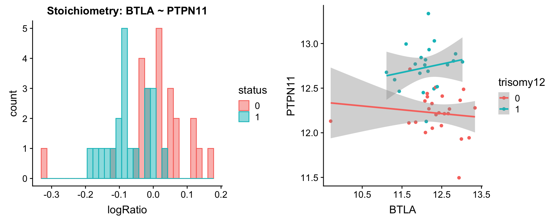
[[5]]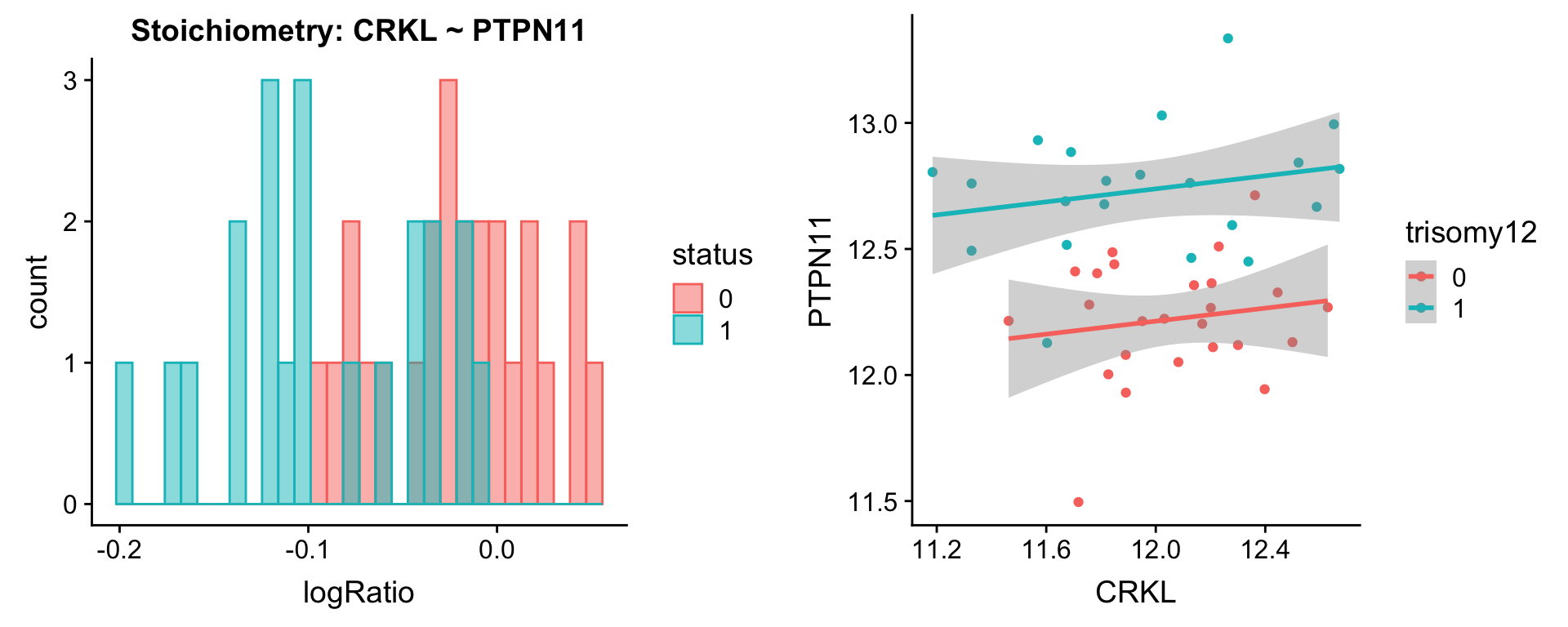
Pairs involving STAT2
protList <- c("STAT2")
plotPair.rna(comRes.pqr, protList, ddsSub.vst, "trisomy12")
[[1]]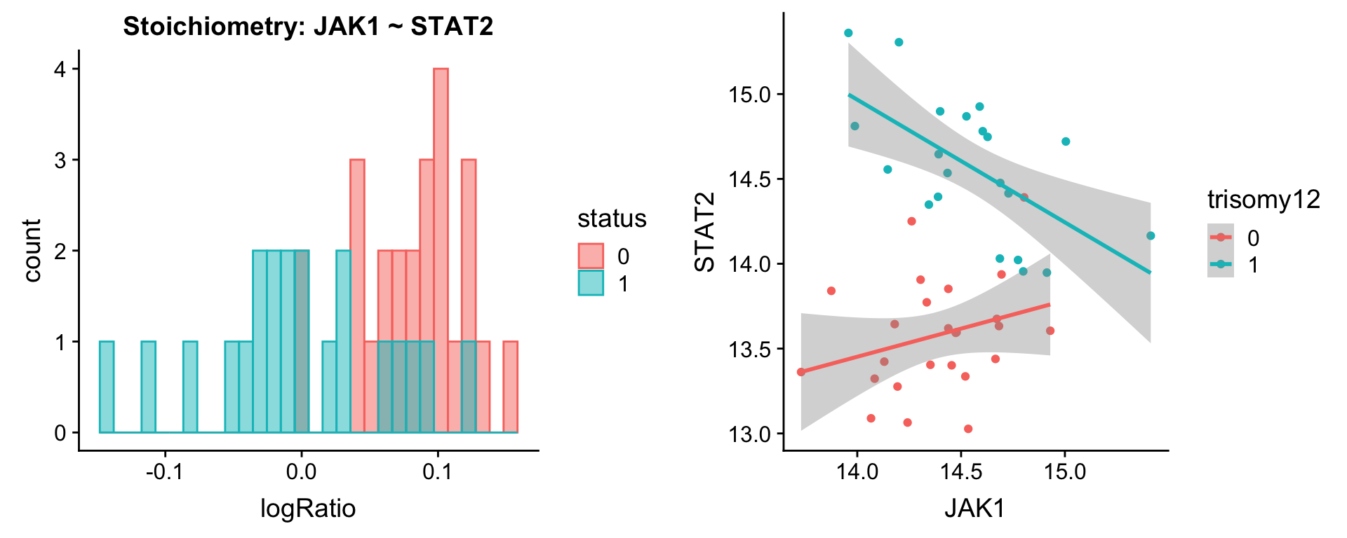
[[2]]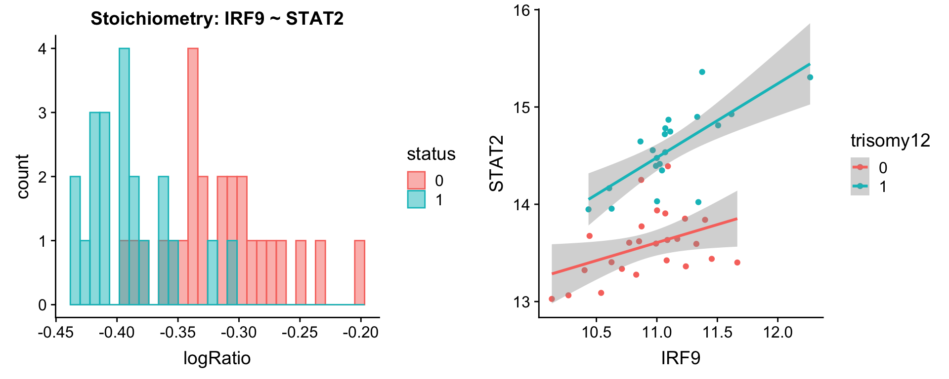
Detect differential complex formations based on correlation test
This approach is based on the hypothesis that if two proteins are in complexes, there abundance should be correlated among samples. The correlation changes are not affected by simple up-regulation or down-regulation. But the problem of this approach is that one needs a relatively larger sample size to detect real change of correlations. And therefore, this method seems to be two stringent in our dataset. In addition, the change of correlations in protein abundance can also be due to the change of gene expression changes, not necessarily only due to complex changes.
Differential correlation detection using DGCA package
quant_data_all = assays(protCLL)[["QRILC"]]
quant_data_all <- quant_data_all[order(rownames(quant_data_all)),]

tri12 <- protCLL$trisomy12
designMat <- model.matrix(~tri12+0 )
colnames(designMat) <- c("WT","Tri12")
ddcor_res = ddcorAll(inputMat = quant_data_all, design = designMat,
  compare = c("WT", "Tri12"),
  adjust = "BH", heatmapPlot = FALSE, nPerm = 0, nPairs = "all")
Reformat output
comTab <- int_pairs %>%
  mutate(pair = map2_chr(ProtA, ProtB, ~paste0(sort(c(.x, .y)),collapse = "-"))) %>%
  separate(pair, c("Gene1","Gene2"), "-",remove = FALSE) %>%
  select(Gene1, Gene2) %>% mutate(inComplex= TRUE)

allRes <- left_join(ddcor_res, comTab, by = c("Gene1","Gene2")) %>%
  mutate(inComplex = ifelse(is.na(inComplex),FALSE,TRUE))
Distribution of p-values for protein in complexes and not in complexes
ggplot(allRes, aes(x=pValDiff, fill = inComplex)) + geom_histogram() + facet_wrap(~inComplex, scale="free") +
xlim(0,1)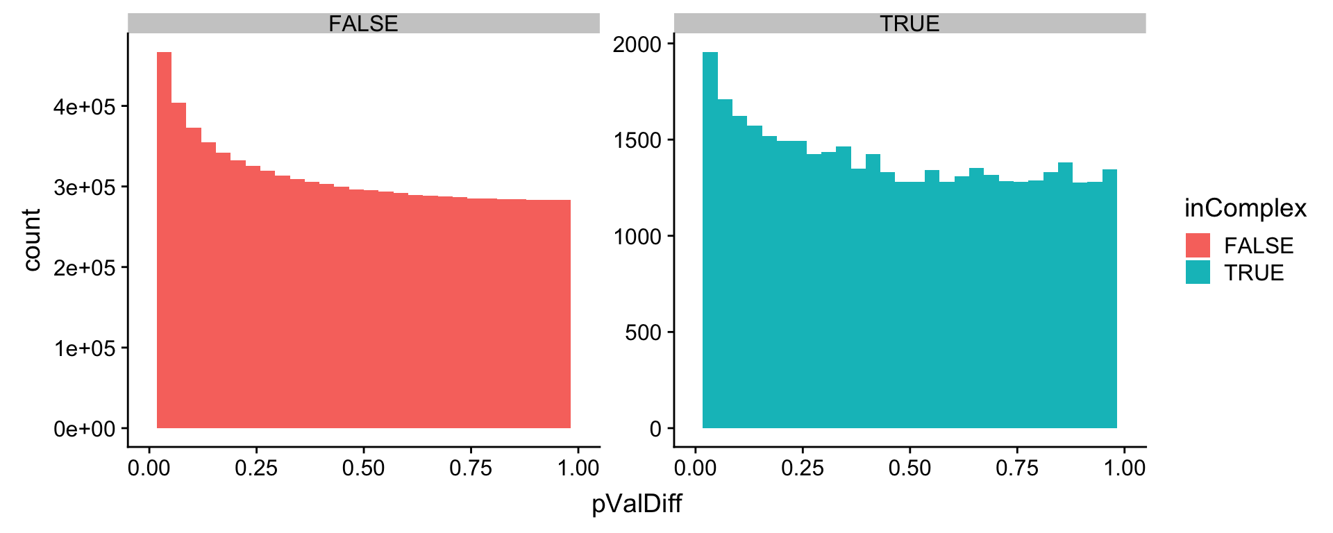 Not much difference.
Differential correlation detection on RNA level
quant_data_all = assay(ddsSub.vst)
quant_data_all <- quant_data_all[order(rownames(quant_data_all)),]

tri12 <- ddsSub.vst$trisomy12
designMat <- model.matrix(~tri12+0 )
colnames(designMat) <- c("WT","Tri12")
ddcor_res = ddcorAll(inputMat = quant_data_all, design = designMat,
  compare = c("WT", "Tri12"),
  adjust = "BH", heatmapPlot = FALSE, nPerm = 0, nPairs = "all")

rnaRes.cor <- ddcor_res %>%
  select(Gene1, Gene2,  pValDiff, pValDiff_adj, Classes) %>%
  dplyr::rename(p.rna = pValDiff, padj.rna = pValDiff_adj, Classes.rna = Classes)
Exploring the results
Only for proteins involved in known complexes
comRes.cor <- filter(allRes, inComplex) %>%
   mutate(protA = rowData(protCLL[Gene1,])$hgnc_symbol,
         protB = rowData(protCLL[Gene2,])$hgnc_symbol,
         chrA = rowData(protCLL[Gene1,])$chromosome_name,
         chrB = rowData(protCLL[Gene2,])$chromosome_name) %>%
  mutate(withChr12 = ifelse(chrA %in% "12" | chrB%in% "12", "yes", "no")) %>% mutate(idx = seq(nrow(.))) %>%
  mutate(p=pValDiff,padj = pValDiff_adj)
Add test results from RNA
comRes.cor <- left_join(comRes.cor, rnaRes.cor, by =c("Gene1","Gene2")) %>%
  mutate(explainedByRNA = ifelse(is.na(p.rna),"no",
                                 ifelse(padj.rna < 0.25 & Classes == Classes.rna,"yes","no")))
P values for pair involving or not involving complex
ggplot(comRes.cor, aes(x=p, fill = withChr12, col = withChr12)) +
  geom_histogram(alpha=0.5, position = "identity", col = NA) + facet_wrap(~withChr12, scale = "free") +
  xlim(0,1)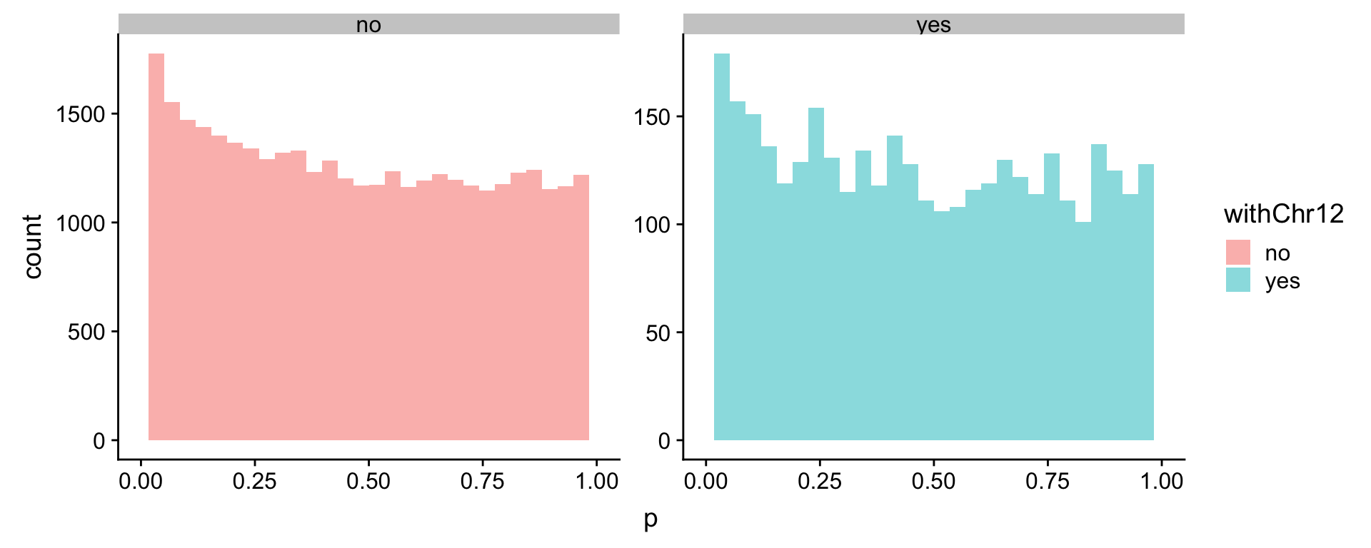
List of significant pairs (25% FDR) As this test is very stringent, I use the looser FDR cut-off here.
comRes.sig <- filter(comRes.cor, withChr12 %in% c("yes")) %>%
  mutate(padj = p.adjust(p, method = "BH"),
         ifSig = padj <0.25) %>%
  filter(ifSig)
comRes.sig %>% select(protA, protB, p, padj, chrA, chrB, withChr12, Classes, explainedByRNA) %>%
  mutate_if(is.numeric, formatC, digits=2, format="e") %>%
DT::datatable() Visualization
Visualize in network plot
comRes.filt <- filter(comRes.sig)
#comRes.filt <- comRes
#get node list
allNodes <- union(comRes.filt$protA, comRes.filt$protB)

nodeList <- data.frame(id = seq(length(allNodes))-1, name = allNodes, stringsAsFactors = FALSE) %>%
  mutate(onChr12 = ifelse(rowData(protCLL[match(name, rowData(protCLL)$hgnc_symbol),])$chromosome_name %in% "12", "chr12","otherChr")) %>%
  mutate(group = corRes.sig[match(name, corRes.sig$name),]$direction) %>%
  mutate(group = ifelse(is.na(group),"ns",group)) %>%
  mutate(nnSize = ifelse(onChr12 == "chr12",100, 1))

#get edge list
edgeList <- select(comRes.filt, protA, protB, p, Classes) %>%
  dplyr::rename(Source = protA, Target = protB) %>%
  mutate(Source = nodeList[match(Source,nodeList$name),]$id,
         Target = nodeList[match(Target, nodeList$name),]$id,
         Classes = as.character(Classes)) %>%
  data.frame(stringsAsFactors = FALSE)

net <- graph_from_data_frame(vertices = nodeList, d=edgeList, directed = FALSE)
Visualize using ggraph
tidyNet <- as_tbl_graph(net)
ggraph(tidyNet) + geom_edge_link(aes(color = Classes), width=1) +
  geom_node_point(aes(color =group, shape = onChr12), size=4) +
  geom_node_text(aes(label = name), repel = TRUE) +
  scale_color_manual(values = c(Up = "pink",Down = "lightblue", ns="grey"))+
theme_graph() 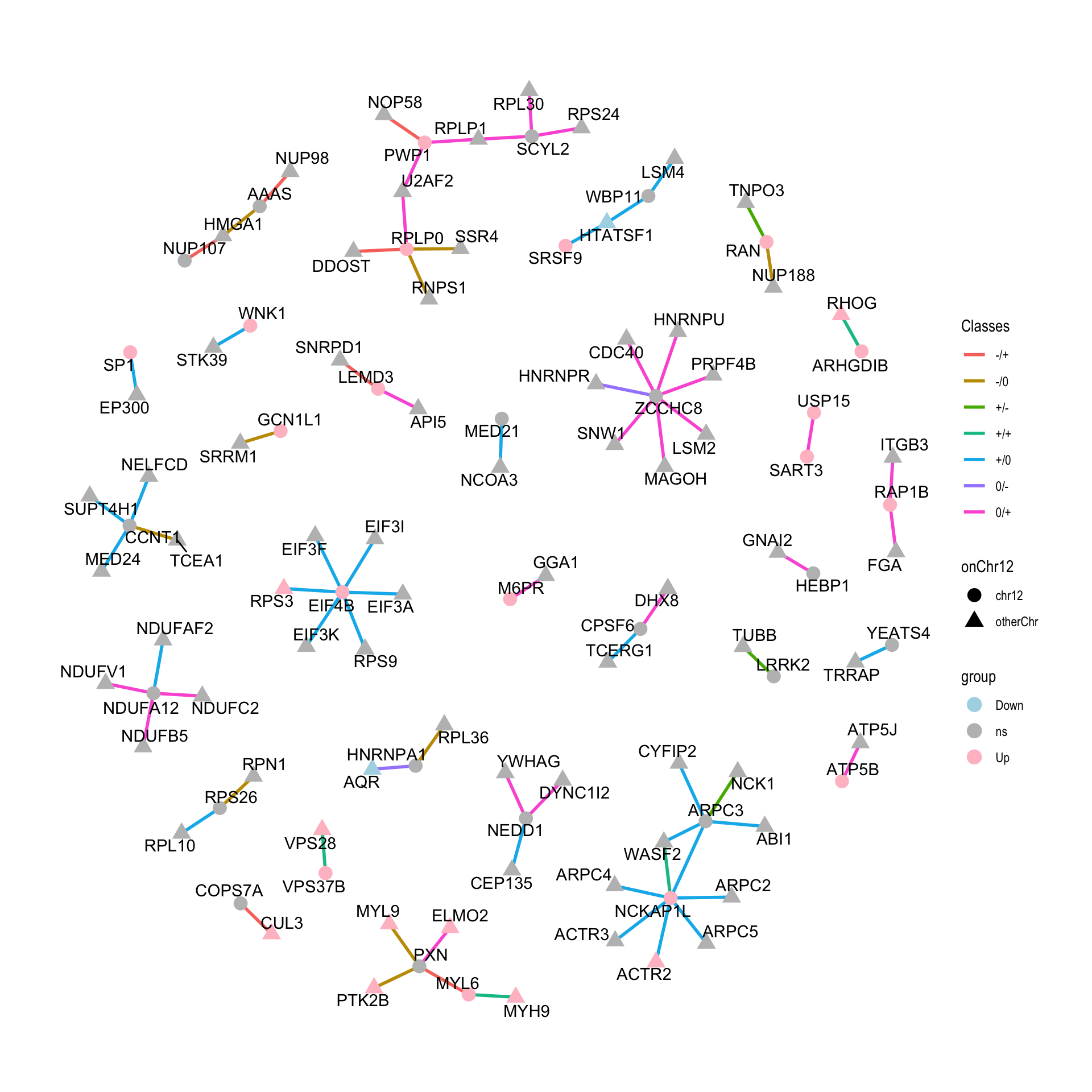
sessionInfo()R version 3.6.0 (2019-04-26)
Platform: x86_64-apple-darwin15.6.0 (64-bit)
Running under: macOS 10.15.4
Matrix products: default
BLAS: /Library/Frameworks/R.framework/Versions/3.6/Resources/lib/libRblas.0.dylib
LAPACK: /Library/Frameworks/R.framework/Versions/3.6/Resources/lib/libRlapack.dylib
locale:
[1] en_US.UTF-8/en_US.UTF-8/en_US.UTF-8/C/en_US.UTF-8/en_US.UTF-8
attached base packages:
[1] parallel stats4 stats graphics grDevices utils datasets
[8] methods base
other attached packages:
[1] forcats_0.4.0 stringr_1.4.0
[3] dplyr_0.8.5 purrr_0.3.3
[5] readr_1.3.1 tidyr_1.0.0
[7] tibble_3.0.0 tidyverse_1.3.0
[9] ggraph_1.0.2 igraph_1.2.4.1
[11] cowplot_0.9.4 ggplot2_3.3.0
[13] DESeq2_1.24.0 proDA_1.1.2
[15] DGCA_1.0.2 tidygraph_1.1.2
[17] SummarizedExperiment_1.14.0 DelayedArray_0.10.0
[19] BiocParallel_1.18.0 matrixStats_0.54.0
[21] Biobase_2.44.0 GenomicRanges_1.36.0
[23] GenomeInfoDb_1.20.0 IRanges_2.18.1
[25] S4Vectors_0.22.0 BiocGenerics_0.30.0
loaded via a namespace (and not attached):
[1] readxl_1.3.1 backports_1.1.4 Hmisc_4.2-0
[4] workflowr_1.6.0 plyr_1.8.4 splines_3.6.0
[7] crosstalk_1.0.0 robust_0.4-18.1 digest_0.6.19
[10] foreach_1.4.4 htmltools_0.4.0 viridis_0.5.1
[13] GO.db_3.8.2 magrittr_1.5 checkmate_2.0.0
[16] memoise_1.1.0 fit.models_0.5-14 cluster_2.1.0
[19] doParallel_1.0.14 fastcluster_1.1.25 annotate_1.62.0
[22] modelr_0.1.5 colorspace_1.4-1 rvest_0.3.5
[25] blob_1.1.1 rrcov_1.4-9 ggrepel_0.8.1
[28] haven_2.2.0 xfun_0.8 crayon_1.3.4
[31] RCurl_1.95-4.12 jsonlite_1.6 genefilter_1.66.0
[34] impute_1.58.0 survival_2.44-1.1 iterators_1.0.10
[37] glue_1.3.2 polyclip_1.10-0 gtable_0.3.0
[40] zlibbioc_1.30.0 XVector_0.24.0 DEoptimR_1.0-8
[43] scales_1.1.0 mvtnorm_1.0-11 DBI_1.0.0
[46] Rcpp_1.0.1 viridisLite_0.3.0 xtable_1.8-4
[49] htmlTable_1.13.1 foreign_0.8-71 bit_1.1-14
[52] preprocessCore_1.46.0 Formula_1.2-3 DT_0.7
[55] htmlwidgets_1.3 httr_1.4.1 RColorBrewer_1.1-2
[58] acepack_1.4.1 ellipsis_0.2.0 pkgconfig_2.0.2
[61] XML_3.98-1.20 farver_2.0.3 nnet_7.3-12
[64] dbplyr_1.4.2 locfit_1.5-9.1 dynamicTreeCut_1.63-1
[67] labeling_0.3 tidyselect_1.0.0 rlang_0.4.5
[70] later_0.8.0 AnnotationDbi_1.46.0 cellranger_1.1.0
[73] munsell_0.5.0 tools_3.6.0 cli_1.1.0
[76] generics_0.0.2 RSQLite_2.1.1 broom_0.5.2
[79] evaluate_0.14 yaml_2.2.0 knitr_1.23
[82] bit64_0.9-7 fs_1.4.0 robustbase_0.93-5
[85] nlme_3.1-140 mime_0.7 xml2_1.2.2
[88] compiler_3.6.0 rstudioapi_0.10 reprex_0.3.0
[91] tweenr_1.0.1 geneplotter_1.62.0 pcaPP_1.9-73
[94] stringi_1.4.3 lattice_0.20-38 Matrix_1.2-17
[97] vctrs_0.2.4 pillar_1.4.3 lifecycle_0.2.0
[100] data.table_1.12.2 bitops_1.0-6 httpuv_1.5.1
[103] R6_2.4.0 latticeExtra_0.6-28 promises_1.0.1
[106] gridExtra_2.3 codetools_0.2-16 MASS_7.3-51.4
[109] assertthat_0.2.1 rprojroot_1.3-2 withr_2.1.2
[112] GenomeInfoDbData_1.2.1 mgcv_1.8-28 hms_0.5.2
[115] grid_3.6.0 rpart_4.1-15 rmarkdown_1.13
[118] git2r_0.26.1 ggforce_0.2.2 shiny_1.3.2
[121] lubridate_1.7.4 WGCNA_1.68 base64enc_0.1-3