Load libraries and dataset

library(SummarizedExperiment)
library(tidygraph)
library(DGCA)
library(proDA)
library(DESeq2)
library(cowplot)
library(igraph)
library(ggraph)
library(tidyverse)

Prepare datasets

load("../output/proteomic_LUMOS_20200430.RData")
load("../../var/patmeta_200522.RData")
load("../../var/ddsrna_180717.RData")

Preprocessing protein and RNA data

#subset samples and genes
overSampe <- intersect(colnames(dds), colnames(protCLL))
overGene <- intersect(rownames(dds), rowData(protCLL)$ensembl_gene_id)
ddsSub <- dds[overGene, overSampe]
protSub <- protCLL[match(overGene, rowData(protCLL)$ensembl_gene_id),overSampe]
rowData(ddsSub)$uniprotID <- rownames(protSub)[match(rownames(ddsSub),rowData(protSub)$ensembl_gene_id)]

#vst
ddsSub.vst <- varianceStabilizingTransformation(ddsSub)

Processing protein complex data

int_pairs <- read_delim("../data/proteins_in_complexes", delim = "\t") %>%
  mutate(Reactome = grepl("Reactome",Evidence_supporting_the_interaction),
         Corum = grepl("Corum",Evidence_supporting_the_interaction)) %>%
  filter(ProtA %in% rownames(protSub) & ProtB %in% rownames(protSub)) %>%
  mutate(pair=map2_chr(ProtA, ProtB, ~paste0(sort(c(.x,.y)), collapse = "-"))) %>%
  mutate(database = case_when(
    Reactome & Corum ~ "both",
    Reactome & !Corum ~ "Reactome",
    !Reactome & Corum ~ "Corum",
    TRUE ~ "other"
  )) %>% mutate(inComplex = "yes")

Differential protein and RNA expression analysis related to trisomy12

fdrCut <- 0.1
exprMat <- assays(protCLL)[["count"]]
designMat <- data.frame(row.names  = colnames(protCLL), IGHV = protCLL$IGHV.status, trisomy12 = protCLL$trisomy12)
fit <- proDA(exprMat, design = ~ .,
             col_data = designMat)

protRes <- test_diff(fit, "trisomy121") %>%
    dplyr::rename(uniprotID = name, logFC = diff, 
                  pvalue = pval, padj = adj_pval) %>% 
    mutate(name = rowData(protCLL[uniprotID,])$hgnc_symbol,
           chrom = rowData(protCLL[uniprotID,])$chromosome_name,
           geneID = rowData(protCLL[uniprotID,])$ensembl_gene_id) %>%
    select(name, uniprotID, geneID, chrom, logFC, pvalue, padj) %>%  
    arrange(pvalue) %>% as_tibble() 

ddsSub$trisomy12 <- patMeta[match(ddsSub$PatID,patMeta$Patient.ID),]$trisomy12
ddsSub$IGHV <- patMeta[match(ddsSub$PatID, patMeta$Patient.ID),]$IGHV.status
design(ddsSub) <- ~ trisomy12 + IGHV
deRes <- DESeq(ddsSub, betaPrior = TRUE)
rnaRes <- results(deRes, name = "trisomy121", tidy = TRUE) %>%
  dplyr::rename(geneID = row, log2FC.rna = log2FoldChange, 
                pvalue.rna = pvalue, padj.rna = padj) %>%
  select(geneID, log2FC.rna, pvalue.rna, padj.rna)

allRes <- left_join(protRes, rnaRes, by = "geneID")

Construct protein-protein interaction network by connecting chr12 proteins and non-chr12 protein

comTab <- int_pairs %>% select(ProtA, ProtB, database) %>%
  mutate(chrA = rowData(protCLL[ProtA,])$chromosome_name,
         chrB = rowData(protCLL[ProtB,])$chromosome_name) %>%
  filter(!is.na(chrA), !is.na(chrB)) %>%
  filter((chrA == "12" & chrB != "12") | (chrA !="12" & chrB == "12")) %>%
  mutate(source = ifelse(chrA == 12, ProtA, ProtB),
         target = ifelse(chrA == 12, ProtB, ProtA)) %>%
  select(source, target, database)

fdrCut <- 0.1
resTab <- select(allRes, name, uniprotID, chrom, padj, padj.rna, logFC,log2FC.rna) %>%
  mutate(sigProt = padj <= fdrCut,
         sigRna = padj.rna <=fdrCut,
         upProt = sigProt & logFC > 0,
         upRna = sigRna & log2FC.rna > 0)
comTab <- comTab %>% 
  left_join(resTab, by = c(source = "uniprotID")) %>%
  left_join(resTab, by = c(target = "uniprotID")) %>%
  rename_all(funs(str_replace(., "x", "source"))) %>%
  rename_all(funs(str_replace(., "y", "target"))) 

comTab.filter <- filter(comTab, sigProt.source, sigProt.target, !sigRna.target, upProt.source, upProt.target)

#get node list
allNodes <- union(comTab.filter$name.source, comTab.filter$name.target) 

nodeList <- data.frame(id = seq(length(allNodes))-1, name = allNodes, stringsAsFactors = FALSE) %>%
  mutate(onChr12 = ifelse(rowData(protCLL[match(name, rowData(protCLL)$hgnc_symbol),])$chromosome_name %in% "12", 
                          "chr12","otherChr"))

#get edge list
edgeList <- select(comTab.filter, name.source, name.target, database) %>%
  dplyr::rename(Source = name.source, Target = name.target) %>% 
  mutate(Source = nodeList[match(Source,nodeList$name),]$id,
         Target = nodeList[match(Target, nodeList$name),]$id) %>%
  data.frame(stringsAsFactors = FALSE)

net <- graph_from_data_frame(vertices = nodeList, d=edgeList, directed = FALSE)

tidyNet <- as_tbl_graph(net)
ggraph(tidyNet) + geom_edge_link(aes(color = database), width=1) + 
  geom_node_point(aes(color =onChr12, shape = onChr12), size=5) + 
  geom_node_text(aes(label = name), repel = TRUE) +
  scale_color_manual(values = c(chr12 = "red",otherChr = "blue")) +
  scale_edge_color_brewer(palette = "Set2") +
  theme_graph()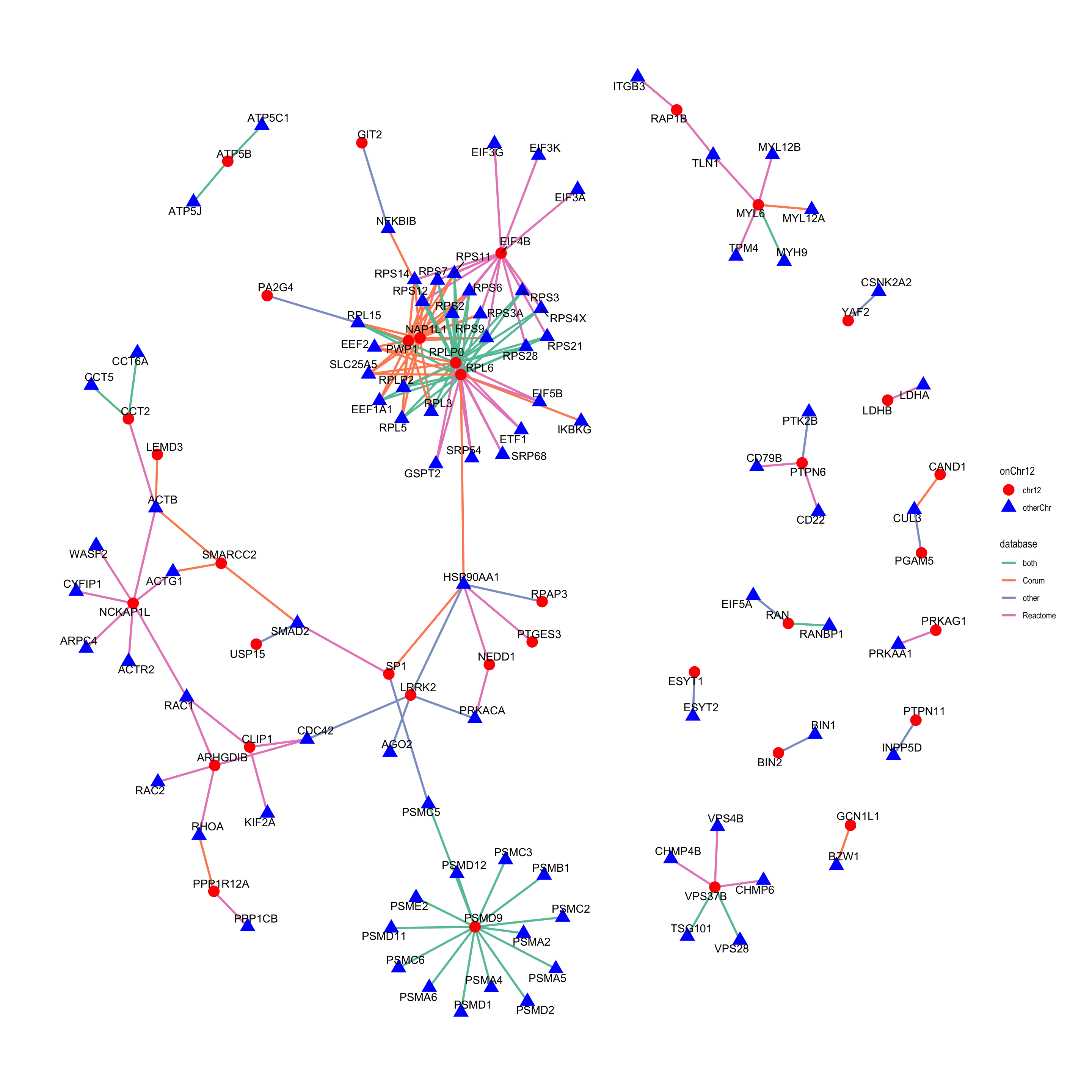 

In this plot, the proteins on chr12 are shown as red circles and non-chr12 proteins are blue triangles. The color of the edges indicate the databases that the complexes based upon. I consider “both” (annotated both in Corum and Reactome) as the stronger evidence, while “other” (not annotated in either Corum or Reactome database but some other databases) as weaker evidence. But this is very subjective.

I think it’s easier to interpret this network. For example, there’s a module center by a chr12 gene PTPN6, which involves CD79B, CD22, PTK2B. This module can be explained as that, trisomy12 leads to the up-regulation of PTPN6 at protein level, which in turn leads to the up-regulation of CD79B, CD22 and PTK2B in trisomy12 samples. This observation is more likely explained by the stabilizing effect through forming complex among those proteins rather than by RNA expressions, as the RNA expression levels of CD79B, CD22, PTK2B are not different between trisomy12 and WT samples.

I also find the clusters of this network quite interesting: There’s one large cluster involving protein synthesis pathways (ribosome, eIF) centered around three chr12 proteins: RPLP0, RPL6 and eIF4B, which may indicate trisomy12 regulate protein synthesis through propagating gene dosage effect by this complex. There are also some clusters involving proteosome complexes (PSMD9), motor proteins (MYL6), PTPN6/PTPN11 and so on. They are potentially interesting. Let me know if there are some candidates you want to investigate further.

PTPN11-INPP5D

protList <- c("PTPN11","INPP5D")

plotSubNet <- function(protList,edgeTab, nodeTab) {
  #get node list
  subCom <- filter(edgeTab, nameA %in% protList | nameB %in% protList)
  allNodes <- union(subCom$nameA, subCom$nameB) 
   
  nodeList <- data.frame(id = seq(length(allNodes))-1, name = allNodes, stringsAsFactors = FALSE) %>%
    left_join(nodeTab, by = "name") %>%
    mutate(onChr12 = ifelse(chrom %in% "12", 
                            "chr12","otherChr"))
  
  #get edge list
  edgeList <- select(subCom, nameA, nameB, database) %>%
    dplyr::rename(Source = nameA, Target = nameB) %>% 
    mutate(Source = nodeList[match(Source,nodeList$name),]$id,
           Target = nodeList[match(Target, nodeList$name),]$id) %>%
    data.frame(stringsAsFactors = FALSE)
  
  net <- graph_from_data_frame(vertices = nodeList, d=edgeList, directed = FALSE)
  
  tidyNet <- as_tbl_graph(net)
ggraph(tidyNet) + geom_edge_link(aes(color = database), width=1) + 
  geom_node_point(aes(color =group, shape = onChr12), size=5) + 
  geom_node_text(aes(label = name), repel = TRUE) +
  scale_color_manual(values = c(both_up = "red", Protein_up = "blue", RNA_up = "orange", none = "grey")) +
  scale_edge_color_brewer(palette = "Set2") +
  theme_graph() 

}

plotSubNet(protList,edgeTab, nodeTab)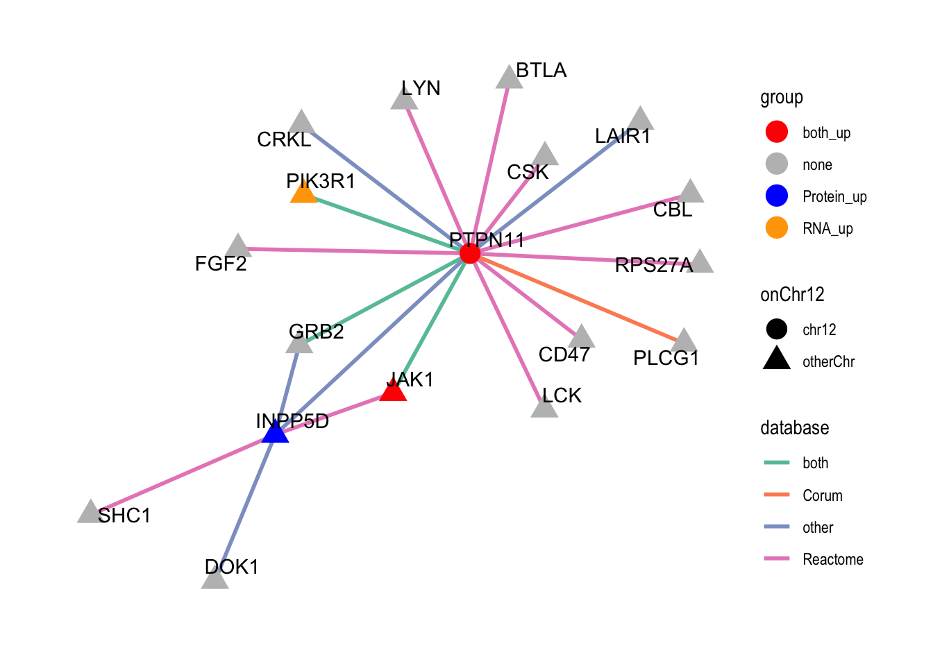

This network plot is similar as above, but focus on the pair PTPN11 and INPP5D. Gene that do not show significant expression changes at protein or RNA levels were also included.

PTPN6-CD79B/CD22/PTK2B

protList <- c("PTPN6","CD79B","CD22","PTK2B")

plotSubNet(protList,edgeTab, nodeTab)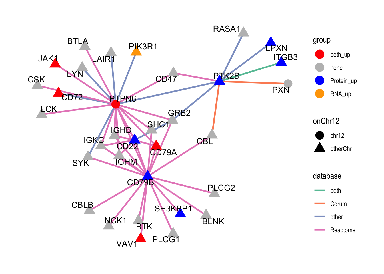

Session information

sessionInfo()

R version 3.6.0 (2019-04-26)
Platform: x86_64-apple-darwin15.6.0 (64-bit)
Running under: macOS  10.15.4

Matrix products: default
BLAS:   /Library/Frameworks/R.framework/Versions/3.6/Resources/lib/libRblas.0.dylib
LAPACK: /Library/Frameworks/R.framework/Versions/3.6/Resources/lib/libRlapack.dylib

locale:
[1] en_US.UTF-8/en_US.UTF-8/en_US.UTF-8/C/en_US.UTF-8/en_US.UTF-8

attached base packages:
[1] parallel  stats4    stats     graphics  grDevices utils     datasets 
[8] methods   base     

other attached packages:
 [1] forcats_0.4.0               stringr_1.4.0              
 [3] dplyr_0.8.5                 purrr_0.3.3                
 [5] readr_1.3.1                 tidyr_1.0.0                
 [7] tibble_3.0.0                tidyverse_1.3.0            
 [9] ggraph_1.0.2                igraph_1.2.4.1             
[11] cowplot_0.9.4               ggplot2_3.3.0              
[13] DESeq2_1.24.0               proDA_1.1.2                
[15] DGCA_1.0.2                  tidygraph_1.1.2            
[17] SummarizedExperiment_1.14.0 DelayedArray_0.10.0        
[19] BiocParallel_1.18.0         matrixStats_0.54.0         
[21] Biobase_2.44.0              GenomicRanges_1.36.0       
[23] GenomeInfoDb_1.20.0         IRanges_2.18.1             
[25] S4Vectors_0.22.0            BiocGenerics_0.30.0        

loaded via a namespace (and not attached):
  [1] readxl_1.3.1           backports_1.1.4        Hmisc_4.2-0           
  [4] workflowr_1.6.0        plyr_1.8.4             splines_3.6.0         
  [7] robust_0.4-18.1        digest_0.6.19          foreach_1.4.4         
 [10] htmltools_0.4.0        viridis_0.5.1          GO.db_3.8.2           
 [13] magrittr_1.5           checkmate_2.0.0        memoise_1.1.0         
 [16] fit.models_0.5-14      cluster_2.1.0          doParallel_1.0.14     
 [19] fastcluster_1.1.25     annotate_1.62.0        modelr_0.1.5          
 [22] colorspace_1.4-1       rvest_0.3.5            blob_1.1.1            
 [25] rrcov_1.4-9            ggrepel_0.8.1          haven_2.2.0           
 [28] xfun_0.8               crayon_1.3.4           RCurl_1.95-4.12       
 [31] jsonlite_1.6           genefilter_1.66.0      impute_1.58.0         
 [34] survival_2.44-1.1      iterators_1.0.10       glue_1.3.2            
 [37] polyclip_1.10-0        gtable_0.3.0           zlibbioc_1.30.0       
 [40] XVector_0.24.0         DEoptimR_1.0-8         scales_1.1.0          
 [43] mvtnorm_1.0-11         DBI_1.0.0              Rcpp_1.0.1            
 [46] viridisLite_0.3.0      xtable_1.8-4           htmlTable_1.13.1      
 [49] foreign_0.8-71         bit_1.1-14             preprocessCore_1.46.0 
 [52] Formula_1.2-3          htmlwidgets_1.3        httr_1.4.1            
 [55] RColorBrewer_1.1-2     acepack_1.4.1          ellipsis_0.2.0        
 [58] pkgconfig_2.0.2        XML_3.98-1.20          farver_2.0.3          
 [61] nnet_7.3-12            dbplyr_1.4.2           locfit_1.5-9.1        
 [64] dynamicTreeCut_1.63-1  labeling_0.3           tidyselect_1.0.0      
 [67] rlang_0.4.5            later_0.8.0            AnnotationDbi_1.46.0  
 [70] cellranger_1.1.0       munsell_0.5.0          tools_3.6.0           
 [73] cli_1.1.0              generics_0.0.2         RSQLite_2.1.1         
 [76] broom_0.5.2            evaluate_0.14          yaml_2.2.0            
 [79] knitr_1.23             bit64_0.9-7            fs_1.4.0              
 [82] robustbase_0.93-5      nlme_3.1-140           xml2_1.2.2            
 [85] compiler_3.6.0         rstudioapi_0.10        reprex_0.3.0          
 [88] tweenr_1.0.1           geneplotter_1.62.0     pcaPP_1.9-73          
 [91] stringi_1.4.3          lattice_0.20-38        Matrix_1.2-17         
 [94] vctrs_0.2.4            pillar_1.4.3           lifecycle_0.2.0       
 [97] data.table_1.12.2      bitops_1.0-6           httpuv_1.5.1          
[100] R6_2.4.0               latticeExtra_0.6-28    promises_1.0.1        
[103] gridExtra_2.3          codetools_0.2-16       MASS_7.3-51.4         
[106] assertthat_0.2.1       rprojroot_1.3-2        withr_2.1.2           
[109] GenomeInfoDbData_1.2.1 hms_0.5.2              grid_3.6.0            
[112] rpart_4.1-15           rmarkdown_1.13         git2r_0.26.1          
[115] ggforce_0.2.2          lubridate_1.7.4        WGCNA_1.68            
[118] base64enc_0.1-3