Correlate proteomic profiling with genomic background (without blocking for IGHV and trisomy12)
Junyan Lu
2020-03-07
Last updated: 2020-04-24
Checks: 5 2
Knit directory: Proteomics/analysis/
This reproducible R Markdown analysis was created with workflowr (version 1.6.0). The Checks tab describes the reproducibility checks that were applied when the results were created. The Past versions tab lists the development history.
The R Markdown is untracked by Git. To know which version of the R Markdown file created these results, you’ll want to first commit it to the Git repo. If you’re still working on the analysis, you can ignore this warning. When you’re finished, you can run wflow_publish to commit the R Markdown file and build the HTML.
Great job! The global environment was empty. Objects defined in the global environment can affect the analysis in your R Markdown file in unknown ways. For reproduciblity it’s best to always run the code in an empty environment.
The command set.seed(20200227) was run prior to running the code in the R Markdown file. Setting a seed ensures that any results that rely on randomness, e.g. subsampling or permutations, are reproducible.
Great job! Recording the operating system, R version, and package versions is critical for reproducibility.
- unnamed-chunk-7
To ensure reproducibility of the results, delete the cache directory correlateGenomic_noBlock_cache and re-run the analysis. To have workflowr automatically delete the cache directory prior to building the file, set delete_cache = TRUE when running wflow_build() or wflow_publish().
Great job! Using relative paths to the files within your workflowr project makes it easier to run your code on other machines.
Great! You are using Git for version control. Tracking code development and connecting the code version to the results is critical for reproducibility. The version displayed above was the version of the Git repository at the time these results were generated.
Note that you need to be careful to ensure that all relevant files for the analysis have been committed to Git prior to generating the results (you can use wflow_publish or wflow_git_commit). workflowr only checks the R Markdown file, but you know if there are other scripts or data files that it depends on. Below is the status of the Git repository when the results were generated:
Ignored files:
    Ignored:    .DS_Store
    Ignored:    .Rhistory
    Ignored:    .Rproj.user/
    Ignored:    analysis/.DS_Store
    Ignored:    analysis/.Rhistory
    Ignored:    analysis/correlateGenomic_cache/
    Ignored:    analysis/correlateGenomic_noBlock_MCLL_cache/
    Ignored:    analysis/correlateGenomic_noBlock_UCLL_cache/
    Ignored:    analysis/correlateGenomic_noBlock_cache/
    Ignored:    code/.Rhistory
    Ignored:    data/.DS_Store
    Ignored:    output/.DS_Store

Untracked files:
    Untracked:  analysis/analysisSplicing.Rmd
    Untracked:  analysis/analysisTrisomy19.Rmd
    Untracked:  analysis/annotateCNV.Rmd
    Untracked:  analysis/correlateGenomic_PC12adjusted.Rmd
    Untracked:  analysis/correlateGenomic_noBlock.Rmd
    Untracked:  analysis/correlateGenomic_noBlock_MCLL.Rmd
    Untracked:  analysis/correlateGenomic_noBlock_UCLL.Rmd
    Untracked:  analysis/default.css
    Untracked:  analysis/patCNV.csv
    Untracked:  analysis/patCNV.xlsx
    Untracked:  analysis/patSNV.csv
    Untracked:  analysis/peptideValidate.Rmd
    Untracked:  analysis/processPeptides_LUMOS.Rmd
    Untracked:  analysis/style.css
    Untracked:  code/utils.R
    Untracked:  data/190909_CLL_prot_abund_med_norm.tsv
    Untracked:  data/190909_CLL_prot_abund_no_norm.tsv
    Untracked:  data/20190423_Proteom_submitted_samples_bereinigt.xlsx
    Untracked:  data/20191025_Proteom_submitted_samples_final.xlsx
    Untracked:  data/LUMOS/
    Untracked:  data/LUMOS_peptides/
    Untracked:  data/LUMOS_protAnnotation.csv
    Untracked:  data/LUMOS_protAnnotation_fix.csv
    Untracked:  data/SampleAnnotation_cleaned.xlsx
    Untracked:  data/facTab_IC50atLeast3New.RData
    Untracked:  data/gmts/
    Untracked:  data/mapEnsemble.txt
    Untracked:  data/mapSymbol.txt
    Untracked:  data/pyprophet_export_aligned.csv
    Untracked:  data/timsTOF_protAnnotation.csv
    Untracked:  output/LUMOS_processed.RData
    Untracked:  output/dxdCLL.RData
    Untracked:  output/pepCLL_lumos.RData
    Untracked:  output/pepTab_lumos.RData
    Untracked:  output/proteomic_LUMOS_20200227.RData
    Untracked:  output/proteomic_LUMOS_20200320.RData
    Untracked:  output/proteomic_timsTOF_20200227.RData
    Untracked:  output/splicingResults.RData
    Untracked:  output/timsTOF_processed.RData

Unstaged changes:
    Modified:   analysis/_site.yml
    Modified:   analysis/analysisSF3B1.Rmd
    Modified:   analysis/compareProteomicsRNAseq.Rmd
    Modified:   analysis/correlateGenomic.Rmd
    Modified:   analysis/correlateMIR.Rmd
    Modified:   analysis/correlateMethylationCluster.Rmd
    Modified:   analysis/index.Rmd
    Modified:   analysis/predictOutcome.Rmd
    Modified:   analysis/processProteomics_LUMOS.Rmd
    Modified:   analysis/qualityControl_LUMOS.Rmd
Note that any generated files, e.g. HTML, png, CSS, etc., are not included in this status report because it is ok for generated content to have uncommitted changes.
There are no past versions. Publish this analysis with wflow_publish() to start tracking its development.
Preprocessing
Process proteomics data
protMat <- assays(protCLL)[["count"]] #without imputation
protCLL$trisomy12 <- patMeta[match(colnames(protCLL),patMeta$Patient.ID),]$trisomy12
Prepare genomic background
Get Mutations with at least 3 cases
geneMat <-  patMeta[match(colnames(protMat), patMeta$Patient.ID),] %>%
  select(Patient.ID, IGHV.status, del11p:U1) %>%
  mutate_if(is.factor, as.character) %>% mutate(IGHV.status = ifelse(IGHV.status == "M", 1,0)) %>%
  mutate_at(vars(-Patient.ID), as.factor) %>% #assign a few unknown mutated cases to wildtype
  data.frame() %>% column_to_rownames("Patient.ID")


geneMat <- geneMat[,apply(geneMat,2, function(x) sum(x %in% 1, na.rm = TRUE))>=3]
Mutations that will be tested
colnames(geneMat) [1] "IGHV.status" "del11q" "del13q" "del14q" "del17p"
[6] "del5IgH" "IgH_break" "trisomy12" "trisomy19" "ATM"
[11] "BRAF" "DDX3X" "EGR2" "FBXW7" "HIST1H1E"
[16] "KRAS" "NOTCH1" "SF3B1" "TP53" Test if there’s interaction between gene mutations (potential confounders)
chiRes <- lapply(seq(1,ncol(geneMat)-1), function(i) {
  lapply(seq(i+1, ncol(geneMat)), function(j) {
    geneA <- colnames(geneMat)[i]
    geneB <- colnames(geneMat)[j]
    #res <- chisq.test(geneMat[,i],geneMat[,j])
    res <- fisher.test(table(geneMat[,i], geneMat[,j]))
    tibble(geneA = geneA, geneB=geneB, p = res$p.value)
  }) %>% bind_rows()
}) %>% bind_rows() %>% arrange(p) %>%
  filter(p <=0.05)
chiRes
# A tibble: 10 x 3
geneA geneB p
<chr> <chr> <dbl>
1 del5IgH IgH_break 0.00226
2 del17p TP53 0.00710
3 IGHV.status del11q 0.0106
4 DDX3X EGR2 0.0111
5 trisomy12 trisomy19 0.0119
6 IGHV.status DDX3X 0.0219
7 del13q trisomy12 0.0222
8 DDX3X FBXW7 0.0265
9 IGHV.status TP53 0.0488
10 IGHV.status trisomy19 0.0496 Heatmap of mutations
plotMat <- apply(geneMat,2,as.numeric)
rownames(plotMat) <- rownames(geneMat)
plotMat <- data.frame(plotMat)
#A recursive function to sort table
sortTab <- function(sumTab) {
i <- ncol(sumTab)
#print(i)
if (i == 1) {
#print(rownames(sumTab)[order(sumTab[,i])])
return(rownames(sumTab)[order(sumTab[,i])])
}
orderRow <- c(sortTab(sumTab[sumTab[,i] %in% c(0,NA), seq(1,i-1), drop = FALSE]), sortTab(sumTab[sumTab[,i] %in% 1, seq(1,i-1), drop = FALSE]))
return(orderRow)
}
#order columns based on number of samples
plotMat <- plotMat[,order(colSums(plotMat, na.rm = TRUE))]
#sort rows based on completeness
sampleOrder <- sortTab(plotMat)
plotMat <- plotMat[rev(sampleOrder),]
pheatmap(t(plotMat), cluster_rows = FALSE, cluster_cols = FALSE)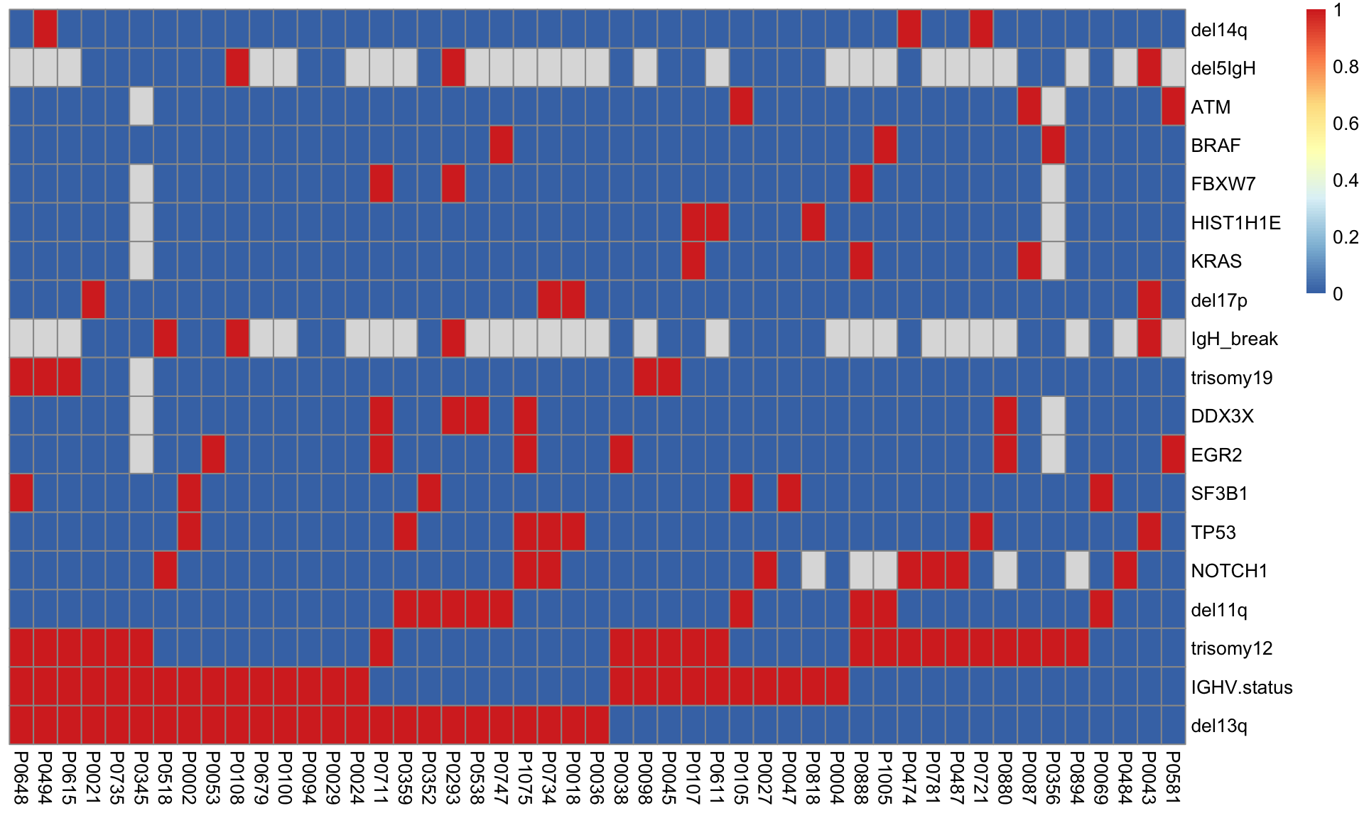 It seems most del11q, NOTCH1, TP53, DDX3X are U-CLLs while most trisomy19 are M-CLL samples.
Test for all variantions (no blocking)
Fit the probailistic dropout model and test for differentially expressed proteins
resList <- lapply(colnames(geneMat), function(n) {
  designMat <- geneMat[,n, drop =FALSE]
  designMat <- designMat[!is.na(designMat[[n]]),,drop=FALSE]
  testMat <- protMat[,rownames(designMat)]

  fit <- proDA(testMat, design = ~ .,
             col_data = designMat)

  contra <- paste0(n,"1")
  resTab <- test_diff(fit, contra) %>%
    dplyr::rename(id = name, logFC = diff, t=t_statistic,
                  P.Value = pval, adj.P.Val = adj_pval) %>%
    mutate(name = rowData(protCLL[id,])$hgnc_symbol) %>%
    select(name, id, logFC, t, P.Value, adj.P.Val) %>%
    arrange(P.Value) %>% mutate(Gene = n) %>%
    as_tibble()
  resTab
}) %>% bind_rows()
P-value histogram for each genomic feature
ggplot(resList, aes(x=P.Value)) + geom_histogram(fill = "green", alpha =0.5, bins=30, col = "grey50") + facet_wrap(~Gene, ncol=4, scales = "fixed") + xlim(0,1)Warning: Removed 38 rows containing missing values (geom_bar).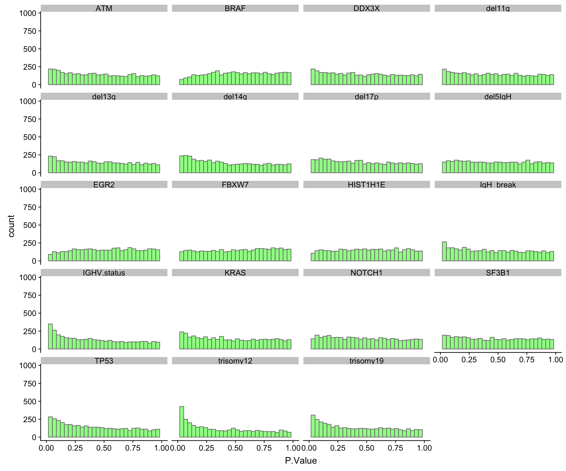
Number of significantly associated proteins at 10% FDR
proNumTab <- resList %>% group_by(Gene) %>%
  summarise(number = sum(adj.P.Val < 0.1, na.rm=TRUE)) %>%
  arrange(desc(number)) %>% mutate(Gene = factor(Gene, levels = Gene))
proNumTab
# A tibble: 19 x 2
Gene number
<fct> <int>
1 trisomy12 1111
2 IGHV.status 336
3 trisomy19 260
4 del11q 30
5 SF3B1 20
6 KRAS 13
7 del14q 12
8 ATM 9
9 del17p 2
10 EGR2 1
11 BRAF 0
12 DDX3X 0
13 del13q 0
14 del5IgH 0
15 FBXW7 0
16 HIST1H1E 0
17 IgH_break 0
18 NOTCH1 0
19 TP53 0Based on the P-value histograms and numbers of significant associations, trisomy12 has the most impact on protein expression, followed by IGHV and del11q. Other genomic variations do not seem to have major impact on protein expression.
Visualize results
IGHV status
List of significant proteins (10% FDR)
corRes.sig <- resList %>% filter(Gene == "IGHV.status", adj.P.Val < 0.1) %>%
  select(-Gene)
corRes.sig %>% mutate_if(is.numeric, formatC, digits=2, format="e") %>% DT::datatable()
Volcano plot
plotVolcano <- function(pTab, fdrCut = 0.05, posCol = "red", negCol = "blue",
                        x_lab = "dm", plotTitle = "",ifLabel = FALSE,
                        colLabel = NULL) {
  plotTab <- pTab %>% mutate(ifSig = ifelse(adj.P.Val > fdrCut, "n.s.",
                                            ifelse(logFC > 0, "up","down"))) %>%
    mutate(ifSig = factor(ifSig, levels = c("up","down","n.s.")))
  pCut <- -log10((filter(plotTab, ifSig != "n.s.") %>% arrange(desc(P.Value)))$P.Value[1])
  g <- ggplot(plotTab, aes(x=logFC, y=-log10(P.Value), label = name)) +
    geom_point(shape = 21, aes(fill = ifSig),size=3) +
    geom_hline(yintercept = pCut, linetype = "dashed") +
    annotate("text", x = -Inf, y = pCut, label = paste0(fdrCut*100,"% FDR"),
             size = 5, vjust = -1.2, hjust=-0.1) +
    scale_fill_manual(values = c(n.s. = "grey70",
                                  up = posCol, down = negCol)) +
    theme( legend.position = "bottom",
          legend.text = element_text(size = 15)) +
    ylab(expression(-log[10]*'('*italic(P)~value*')')) +
    xlab(x_lab) + ggtitle(plotTitle)

  if (ifLabel & is.null(colLabel))
    g <- g + ggrepel::geom_text_repel(data = filter(plotTab, ifSig != "n.s."),
                                      size=5, force = 2)
  else if (ifLabel & !is.null(colLabel)) {
     g <- g+ggrepel::geom_text_repel(data = filter(plotTab, ifSig != "n.s."),
                                    aes_string(col = colLabel),
                                    size=5, force = 2) +
       scale_color_manual(values = c(yes = "red",no = "black"))
  }

  return(g)
}
plotVolcano(filter(resList, Gene == "IGHV.status"), fdrCut =0.01, x_lab="log2FoldChange",
            plotTitle = "IGHV.status", ifLabel = TRUE)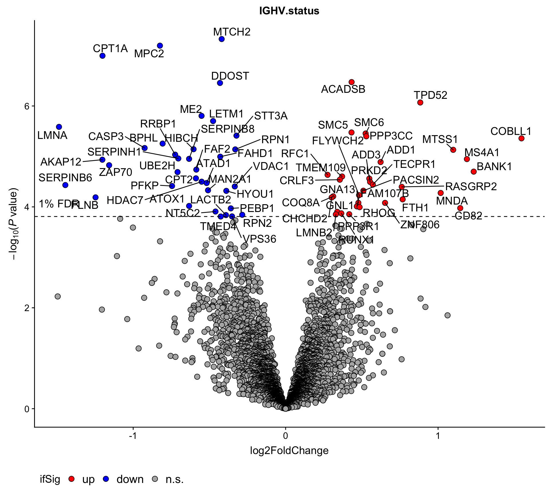
Heatmap of differentially expressed proteins
proList <- corRes.sig$id
plotMat <- assays(protCLL)[["QRILC"]][proList,]
rownames(plotMat) <- rowData(protCLL[proList,])$hgnc_symbol

colAnno <- colData(protCLL)[,c("trisomy12","IGHV.status")] %>%
  data.frame()

plotMat <- jyluMisc::mscale(plotMat, censor = 6)
pheatmap(plotMat, scale = "none", annotation_col = colAnno, clustering_method = "ward.D2",
         color = colorRampPalette(c("navy","white","firebrick"))(100),
         breaks = seq(-6,6, length.out = 101))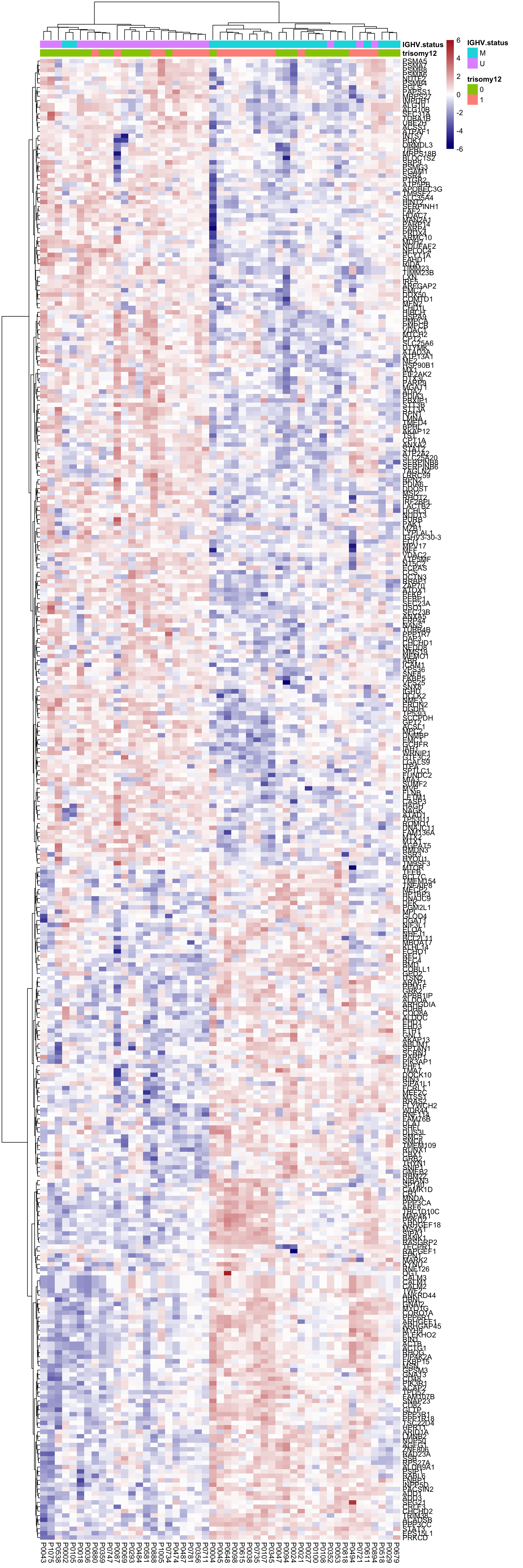
Plot top 9 most differentially expressed proteins
protTab <- sumToTiday(protCLL,"patID") %>% mutate(name = hgnc_symbol)
plotTab <- filter(protTab, name %in% corRes.sig$name[1:9]) %>% dplyr::rename(expression = QRILC)
ggplot(plotTab, aes(x=IGHV.status, y =  expression)) + geom_boxplot(aes(fill = IGHV.status)) + geom_point() +
  facet_wrap(~name, scale = "free")
Enrichment analysis
gmts = list(H= "../data/gmts/h.all.v6.2.symbols.gmt",
            KEGG= "../data/gmts/c2.cp.kegg.v6.2.symbols.gmt")
inputTab <- resList %>% filter(P.Value <0.05, Gene == "IGHV.status") %>%
  mutate(name = rowData(protCLL[id,])$hgnc_symbol) %>% filter(!is.na(name)) %>%
  dplyr::select(name, t) %>% data.frame() %>% column_to_rownames("name")
enRes <- list()
enRes[["HALLMARK"]] <- runGSEA(inputTab, gmts$H, "page")
enRes[["KEGG"]] <- runGSEA(inputTab, gmts$KEGG, "page")
p <- plotEnrichmentBar(enRes, pCut =0.05, ifFDR= FALSE)
Coordinate system already present. Adding new coordinate system, which will replace the existing one.
Coordinate system already present. Adding new coordinate system, which will replace the existing one.plot(p)
Trisomy12
List of significant proteins (10% FDR)
corRes.sig <- resList %>% filter(Gene == "trisomy12", adj.P.Val < 0.1) %>%
  mutate(chromosome = rowData(protCLL[id,])$chromosome_name) %>%
  select(-Gene)
corRes.sig %>% mutate_if(is.numeric, formatC, digits=2, format="e") %>% DT::datatable()
Volcano plot (0.1% FDR)
plotTab <- filter(resList, Gene == "trisomy12") %>%
  mutate(chromosome = rowData(protCLL[id,])$chromosome_name) %>%
  mutate(onChr12 = ifelse(chromosome == "12","yes","no"))
plotVolcano(plotTab, fdrCut =0.001, x_lab="log2FoldChange",
            plotTitle = "trisomy12", ifLabel = TRUE, colLabel = "onChr12")
Labels colored by red indicates the gene is on chromosome 12
Heatmap of differentially expressed proteins (0.1%)
proList <- filter(corRes.sig, !is.na(name),adj.P.Val < 0.001) %>% distinct(name, .keep_all = TRUE) %>% pull(id)
plotMat <- assays(protCLL)[["QRILC"]][proList,]
rownames(plotMat) <- rowData(protCLL[proList,])$hgnc_symbol

colAnno <- colData(protCLL)[,c("gender","trisomy12","IGHV.status")] %>%
  data.frame()

rowAnno <- rowData(protCLL)[proList,c("chromosome_name","hgnc_symbol"),drop=FALSE] %>%
  data.frame(stringsAsFactors = FALSE) %>%
  mutate(onChr12 = ifelse(chromosome_name == "12","yes","no")) %>%
  select(hgnc_symbol, onChr12) %>% data.frame() %>% column_to_rownames("hgnc_symbol")

plotMat <- jyluMisc::mscale(plotMat, censor = 6)

pheatmap(plotMat, scale = "none", annotation_col = colAnno, clustering_method = "ward.D2",
         annotation_row = rowAnno,
         color = colorRampPalette(c("navy","white","firebrick"))(100),
         breaks = seq(-6,6, length.out = 101))
Plot top 9 most differentially expressed proteins
plotTab <- filter(protTab, name %in% corRes.sig$name[1:9]) %>% dplyr::rename(expression = QRILC) %>%
  filter(!is.na(trisomy12))
ggplot(plotTab, aes(x=trisomy12, y =  expression)) + geom_boxplot(aes(fill = trisomy12)) + geom_point() +
  facet_wrap(~name, scale = "free")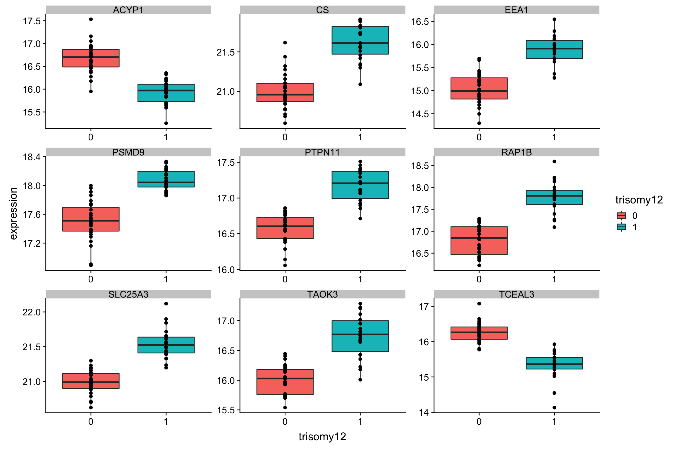
Enrichment analysis
gmts = list(H= "../data/gmts/h.all.v6.2.symbols.gmt",
            KEGG = "../data/gmts/c2.cp.kegg.v6.2.symbols.gmt")
inputTab <- resList %>% filter(P.Value <0.05, Gene == "trisomy12") %>%
  mutate(name = rowData(protCLL[id,])$hgnc_symbol) %>% filter(!is.na(name)) %>%
  distinct(name, .keep_all = TRUE) %>%
  select(name, t) %>% data.frame() %>% column_to_rownames("name")
enRes <- list()
enRes[["HALLMARK"]] <- runGSEA(inputTab, gmts$H, "page")
enRes[["KEGG"]] <- runGSEA(inputTab, gmts$KEGG, "page")
p <- plotEnrichmentBar(enRes, pCut =0.05, ifFDR= FALSE)
Coordinate system already present. Adding new coordinate system, which will replace the existing one.
Coordinate system already present. Adding new coordinate system, which will replace the existing one.#pdf("tri12Enrich.pdf", height = 15, width = 6)
plot(p)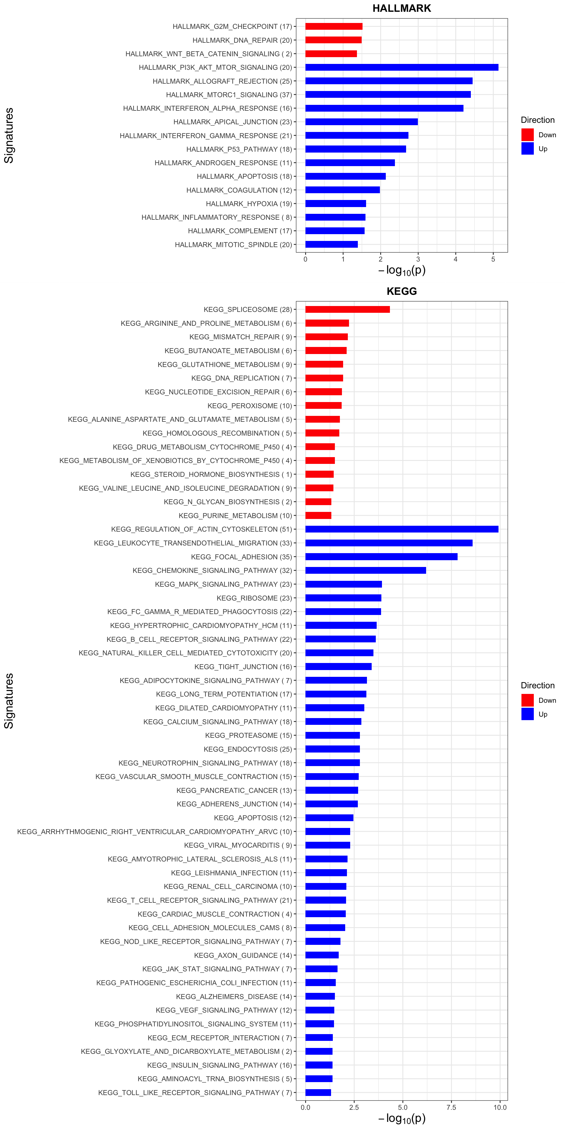
#dev.off()SF3B1
List of significant proteins (10% FDR)
corRes.sig <- resList %>% filter(Gene == "SF3B1", adj.P.Val < 0.1) %>%
  select(-Gene)
corRes.sig %>% mutate_if(is.numeric, formatC, digits=2, format="e") %>% DT::datatable()
Volcano plot
plotVolcano(filter(resList, Gene == "SF3B1"), fdrCut =0.1, x_lab="log2FoldChange",
            plotTitle = "SF3B1", ifLabel = TRUE)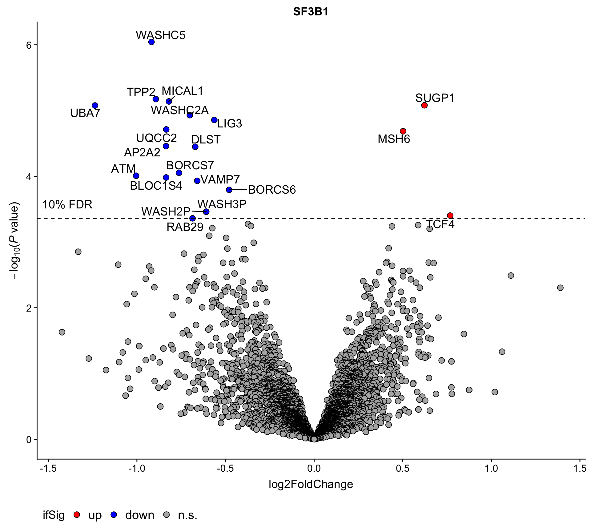
Heatmap of differentially expressed proteins
proList <- corRes.sig$id
plotMat <- assays(protCLL)[["QRILC"]][proList,]
rownames(plotMat) <- rowData(protCLL[proList,])$hgnc_symbol

colAnno <- geneMat[,c("trisomy12","IGHV.status","SF3B1")] %>%
  data.frame()

plotMat <- jyluMisc::mscale(plotMat, censor = 6)
pheatmap(plotMat, scale = "none", annotation_col = colAnno, clustering_method = "ward.D2",
         color = colorRampPalette(c("navy","white","firebrick"))(100),
         breaks = seq(-6,6, length.out = 101))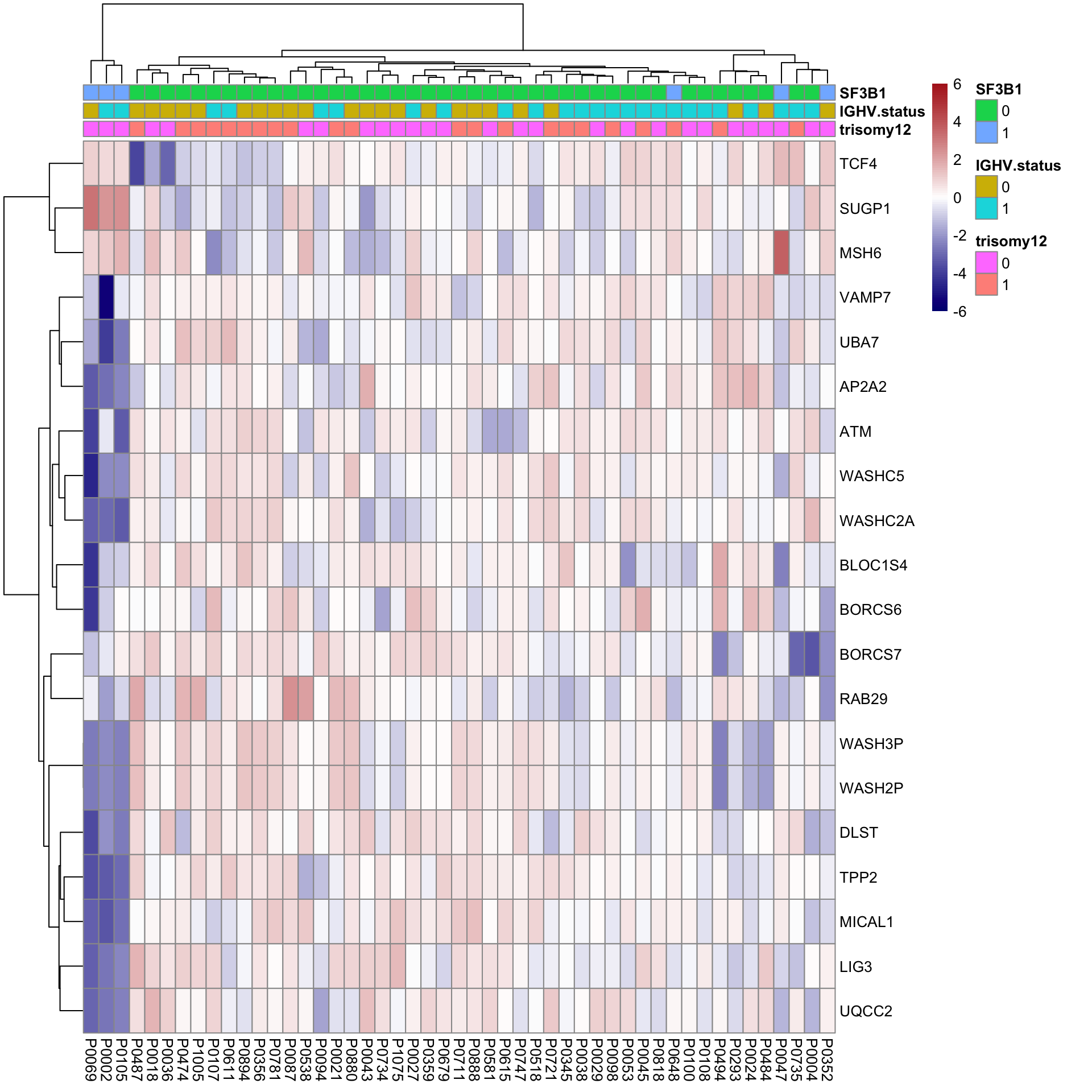
Plot top 9 most differentially expressed proteins
protTab <- sumToTiday(protCLL,"patID") %>% mutate(name = hgnc_symbol)
plotTab <- filter(protTab, name %in% corRes.sig$name[1:9]) %>% dplyr::rename(expression = QRILC) %>%
  mutate(SF3B1 = patMeta[match(colID, patMeta$Patient.ID),]$SF3B1)
ggplot(plotTab, aes(x=SF3B1, y =  expression)) + geom_boxplot(aes(fill = SF3B1)) + geom_point() +
  facet_wrap(~name, scale = "free")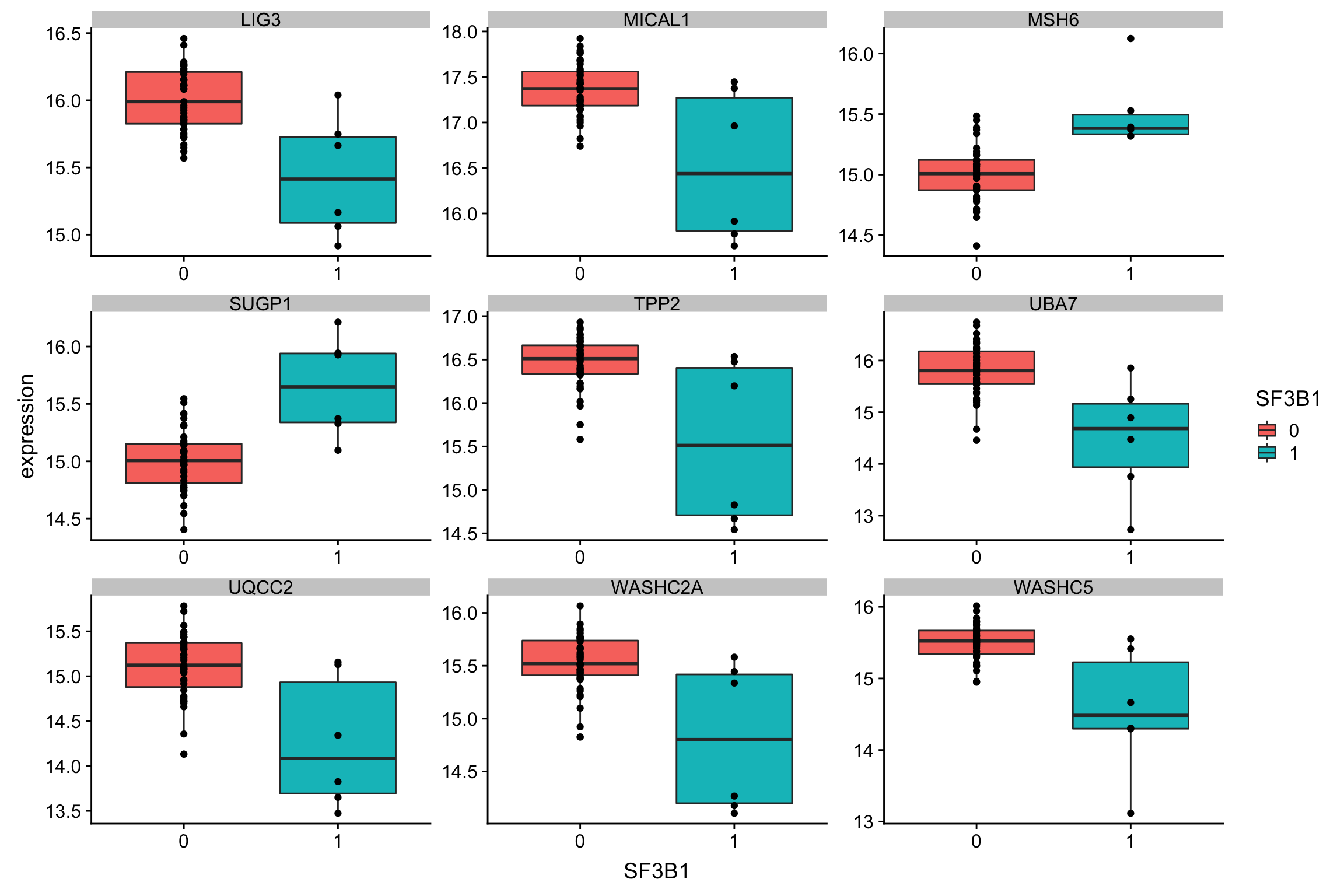
Enrichment analysis
gmts = list(H= "../data/gmts/h.all.v6.2.symbols.gmt",
            KEGG= "../data/gmts/c2.cp.kegg.v6.2.symbols.gmt")
inputTab <- resList %>% filter(P.Value <0.05, Gene == "SF3B1") %>%
  mutate(name = rowData(protCLL[id,])$hgnc_symbol) %>% filter(!is.na(name)) %>%
  dplyr::select(name, t) %>% data.frame() %>% column_to_rownames("name")
enRes <- list()
enRes[["HALLMARK"]] <- runGSEA(inputTab, gmts$H, "page")
enRes[["KEGG"]] <- runGSEA(inputTab, gmts$KEGG, "page")
p <- plotEnrichmentBar(enRes, pCut =0.05, ifFDR= FALSE)
Coordinate system already present. Adding new coordinate system, which will replace the existing one.
Coordinate system already present. Adding new coordinate system, which will replace the existing one.plot(p)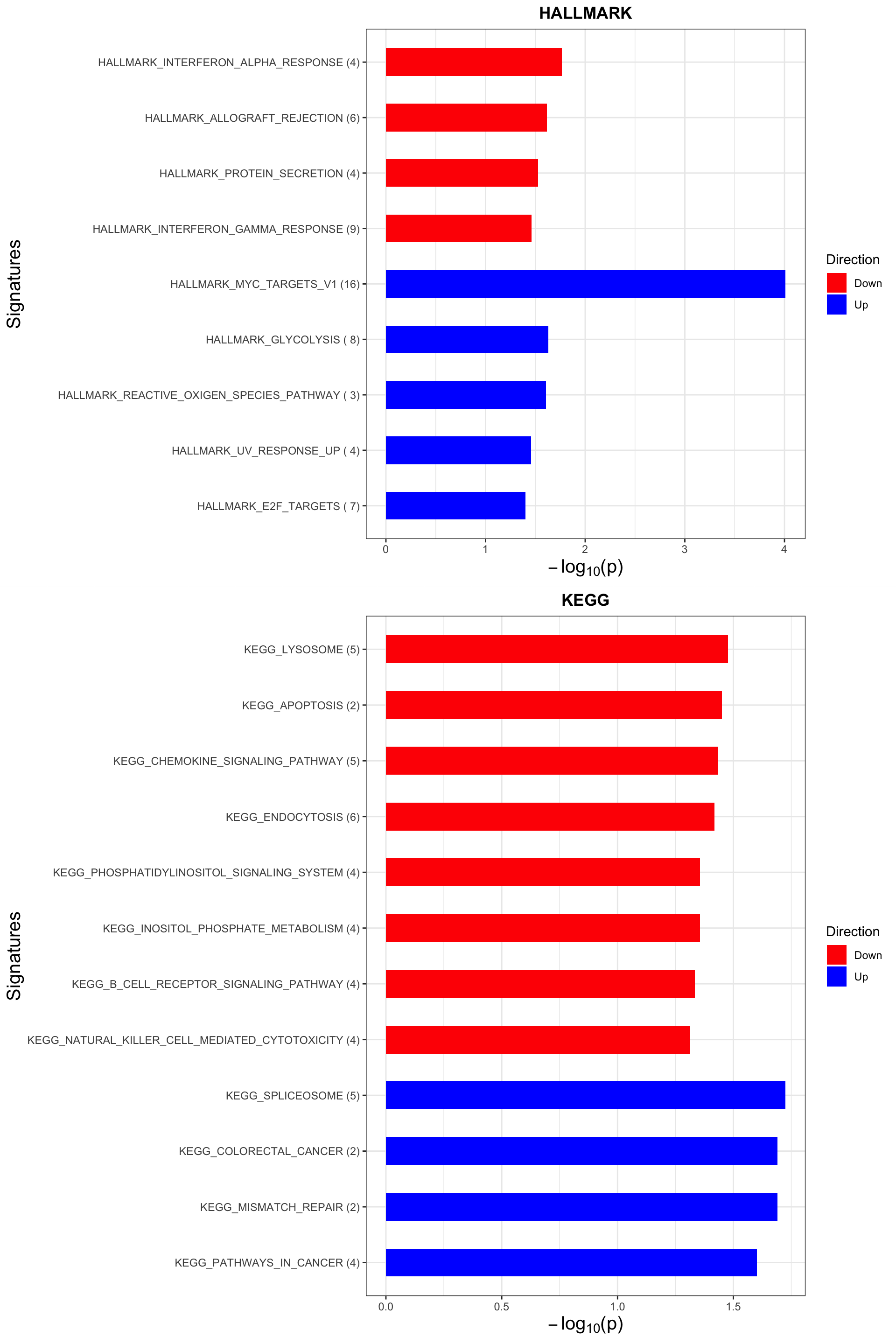
del11q
List of significant proteins (10% FDR)
corRes.sig <- resList %>% filter(Gene == "del11q", adj.P.Val < 0.1) %>%
  mutate(chromosome = rowData(protCLL[id,])$chromosome_name) %>%
  select(-Gene)
corRes.sig %>% mutate_if(is.numeric, formatC, digits=2, format="e") %>% DT::datatable()
Volcano plot
plotTab <- plotTab <- filter(resList, Gene == "del11q") %>%
  mutate(chromosome = rowData(protCLL[id,])$chromosome_name) %>%
  mutate(onChr11 = ifelse(chromosome == "11","yes","no"))
plotVolcano(plotTab, fdrCut =0.1, x_lab="log2FoldChange",
            plotTitle = "del11q", ifLabel = TRUE, colLabel = "onChr11")
Labels colored by red indicates the gene is on chromosome 11
Heatmap of differentially expressed proteins
proList <- filter(corRes.sig, !is.na(name)) %>% distinct(name, .keep_all = TRUE) %>% pull(id)
plotMat <- assays(protCLL)[["QRILC"]][proList,]
rownames(plotMat) <- rowData(protCLL[proList,])$hgnc_symbol

colAnno <- geneMat[,c("del11q","IGHV.status")] %>%
  data.frame()
colAnno$gender <- protCLL[,rownames(colAnno)]$gender

rowAnno <- rowData(protCLL)[proList, c("chromosome_name","hgnc_symbol"),drop=FALSE] %>% data.frame(stringsAsFactors = FALSE) %>%
  mutate(onChr11 = ifelse(chromosome_name == "11","yes","no")) %>%
  select(hgnc_symbol, onChr11) %>% data.frame() %>% column_to_rownames("hgnc_symbol")

plotMat <- jyluMisc::mscale(plotMat, censor = 6)
pheatmap(plotMat, scale = "none", annotation_col = colAnno,  annotation_row = rowAnno,
         clustering_method = "ward.D2",
         color = colorRampPalette(c("navy","white","firebrick"))(100),
         breaks = seq(-6,6, length.out = 101))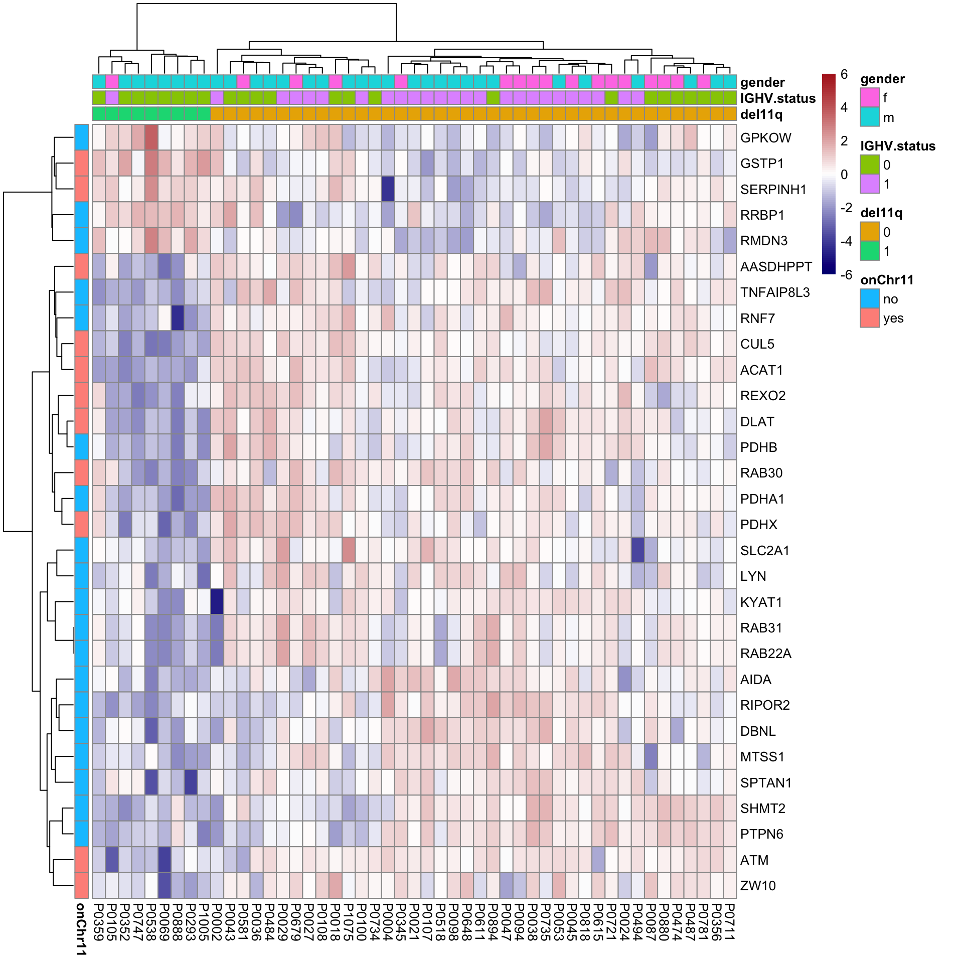
Plot top 9 most differentially expressed proteins
plotTab <- filter(protTab, name %in% corRes.sig$name[1:9]) %>% dplyr::rename(expression = QRILC) %>%
  mutate(del11q = patMeta[match(colID, patMeta$Patient.ID),]$del11q) %>%
  filter(!is.na(del11q))
ggplot(plotTab, aes(x=del11q, y =  expression)) + geom_boxplot(aes(fill = del11q)) + geom_point() +
  facet_wrap(~name, scale = "free")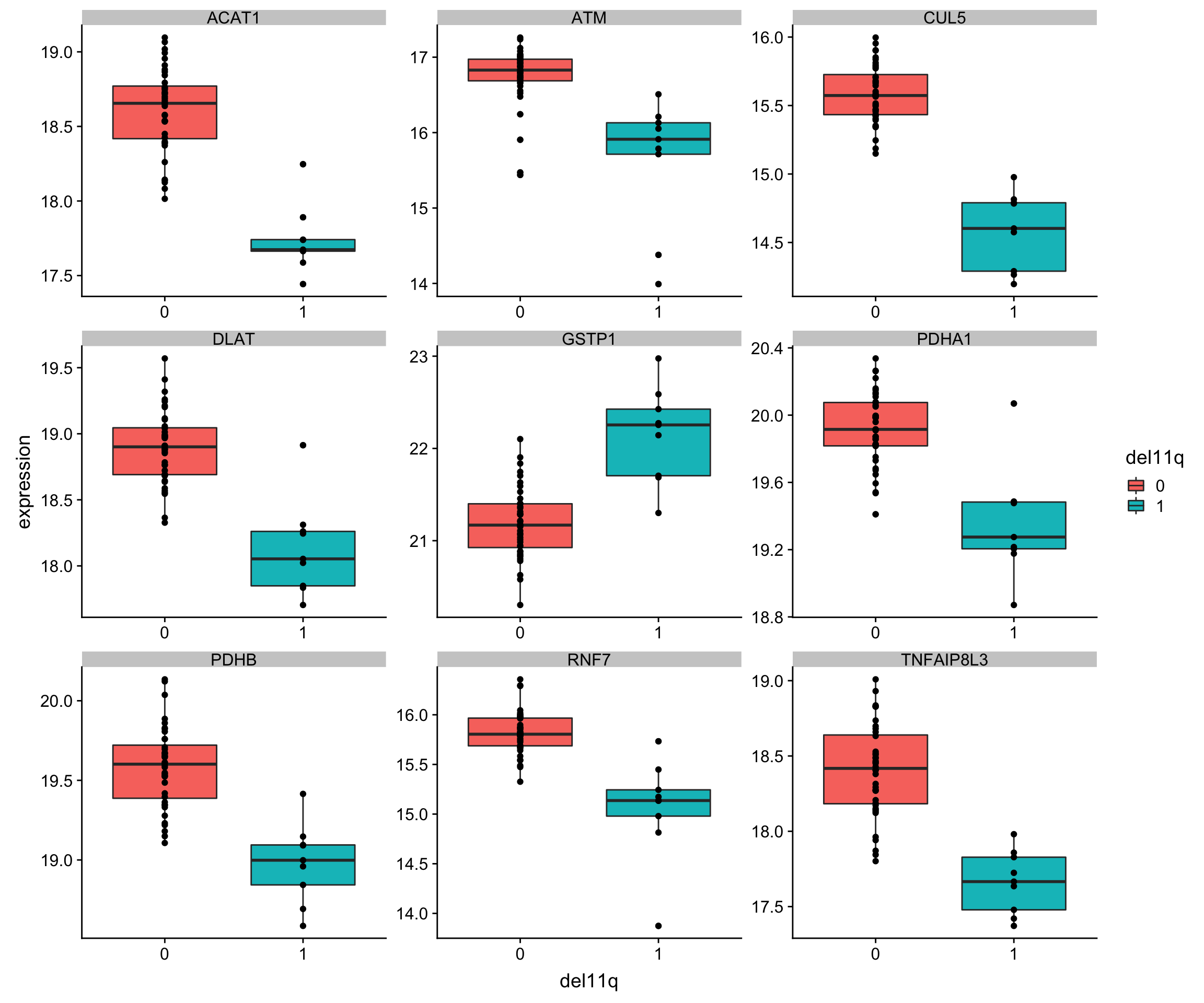
Enrichment analysis
inputTab <- resList %>% filter(P.Value <0.05, Gene == "del11q") %>%
  mutate(name = rowData(protCLL[id,])$hgnc_symbol) %>% filter(!is.na(name)) %>%
  distinct(name, .keep_all = TRUE) %>%
  select(name, t) %>% data.frame() %>% column_to_rownames("name")
enRes <- list()
enRes[["HALLMARK"]] <- runGSEA(inputTab, gmts$H, "page")
enRes[["KEGG"]] <- runGSEA(inputTab, gmts$KEGG, "page")
p <- plotEnrichmentBar(enRes, pCut =0.05, ifFDR= FALSE)
Coordinate system already present. Adding new coordinate system, which will replace the existing one.
Coordinate system already present. Adding new coordinate system, which will replace the existing one.#pdf("tri12Enrich.pdf", height = 15, width = 6)
plot(p)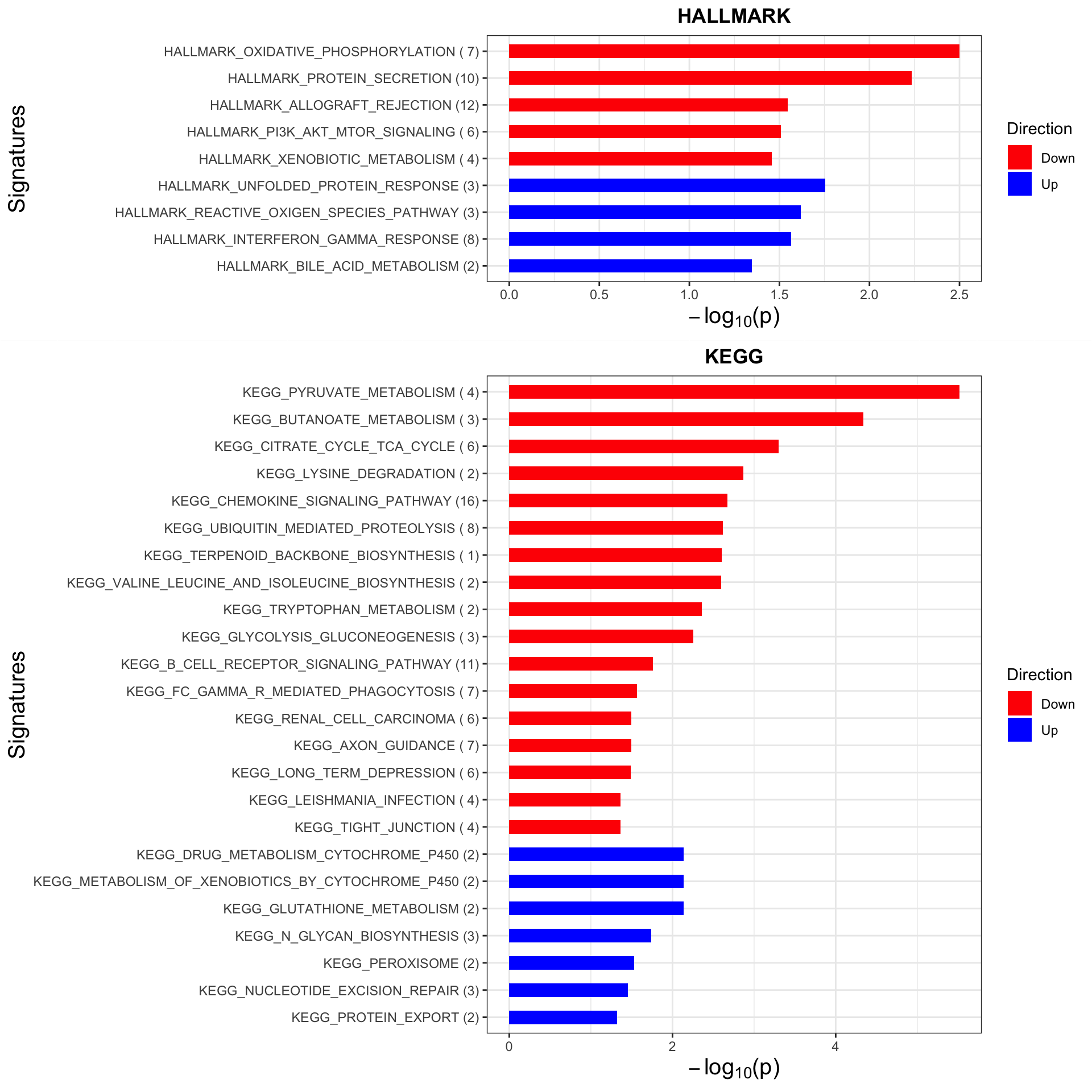
#dev.off()trisomy19
List of significant proteins (10% FDR)
corRes.sig <- resList %>% filter(Gene == "trisomy19", adj.P.Val < 0.1) %>%
  mutate(chromosome = rowData(protCLL[id,])$chromosome_name) %>%
  select(-Gene)
corRes.sig %>% mutate_if(is.numeric, formatC, digits=2, format="e") %>% DT::datatable()
Volcano plot
plotTab <- plotTab <- filter(resList, Gene == "trisomy19") %>%
mutate(chromosome = rowData(protCLL[id,])$chromosome_name) %>%
mutate(onChr19 = ifelse(chromosome == "19","yes","no"))
plotVolcano(plotTab, fdrCut =0.1, x_lab="log2FoldChange",
plotTitle = "trisomy19", ifLabel = TRUE, colLabel = "onChr19")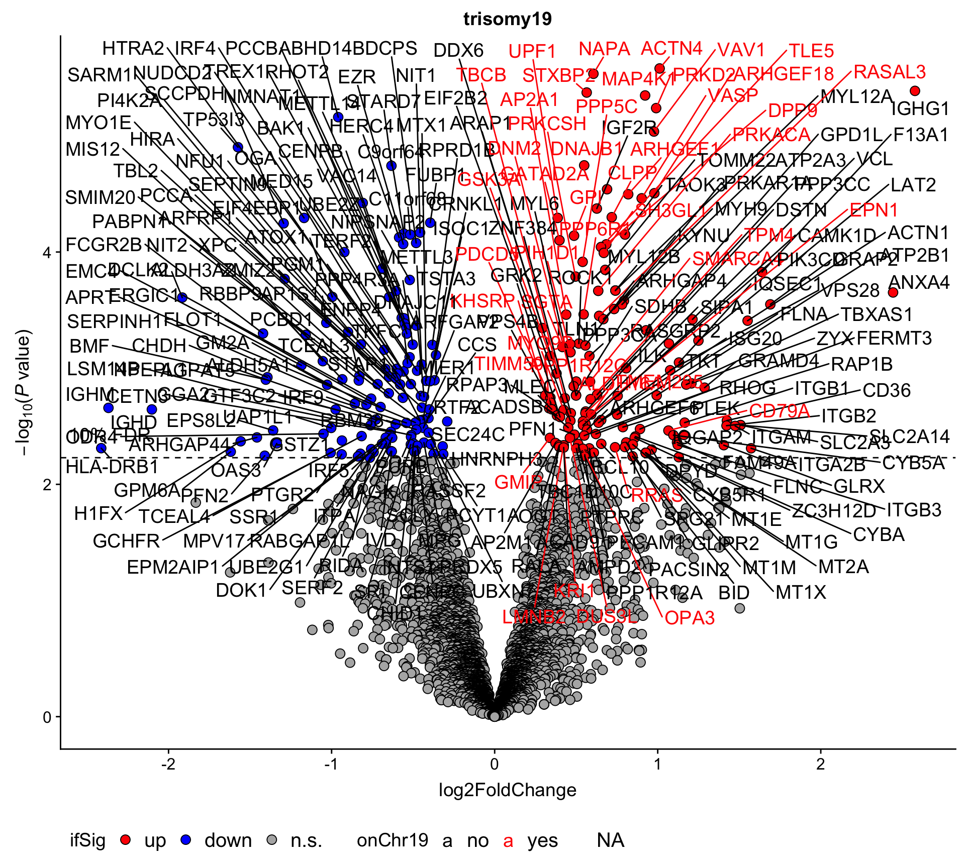 Labels colored by red indicates the gene is on chromosome 19
Heatmap of differentially expressed proteins
proList <- filter(corRes.sig, !is.na(name)) %>% distinct(name, .keep_all = TRUE) %>% pull(id)
plotMat <- assays(protCLL)[["QRILC"]][proList,]
rownames(plotMat) <- rowData(protCLL[proList,])$hgnc_symbol

colAnno <- geneMat[,c("trisomy19","IGHV.status","trisomy12")] %>%
  data.frame()

rowAnno <- rowData(protCLL)[proList, c("chromosome_name","hgnc_symbol"),drop=FALSE] %>% data.frame(stringsAsFactors = FALSE) %>%
  mutate(onChr19 = ifelse(chromosome_name == "19","yes","no")) %>%
  select(hgnc_symbol, onChr19) %>% data.frame() %>% column_to_rownames("hgnc_symbol")

plotMat <- jyluMisc::mscale(plotMat, censor = 6)
pheatmap(plotMat, scale = "none", annotation_col = colAnno,  annotation_row = rowAnno,
         clustering_method = "ward.D2",
         color = colorRampPalette(c("navy","white","firebrick"))(100),
         breaks = seq(-6,6, length.out = 101))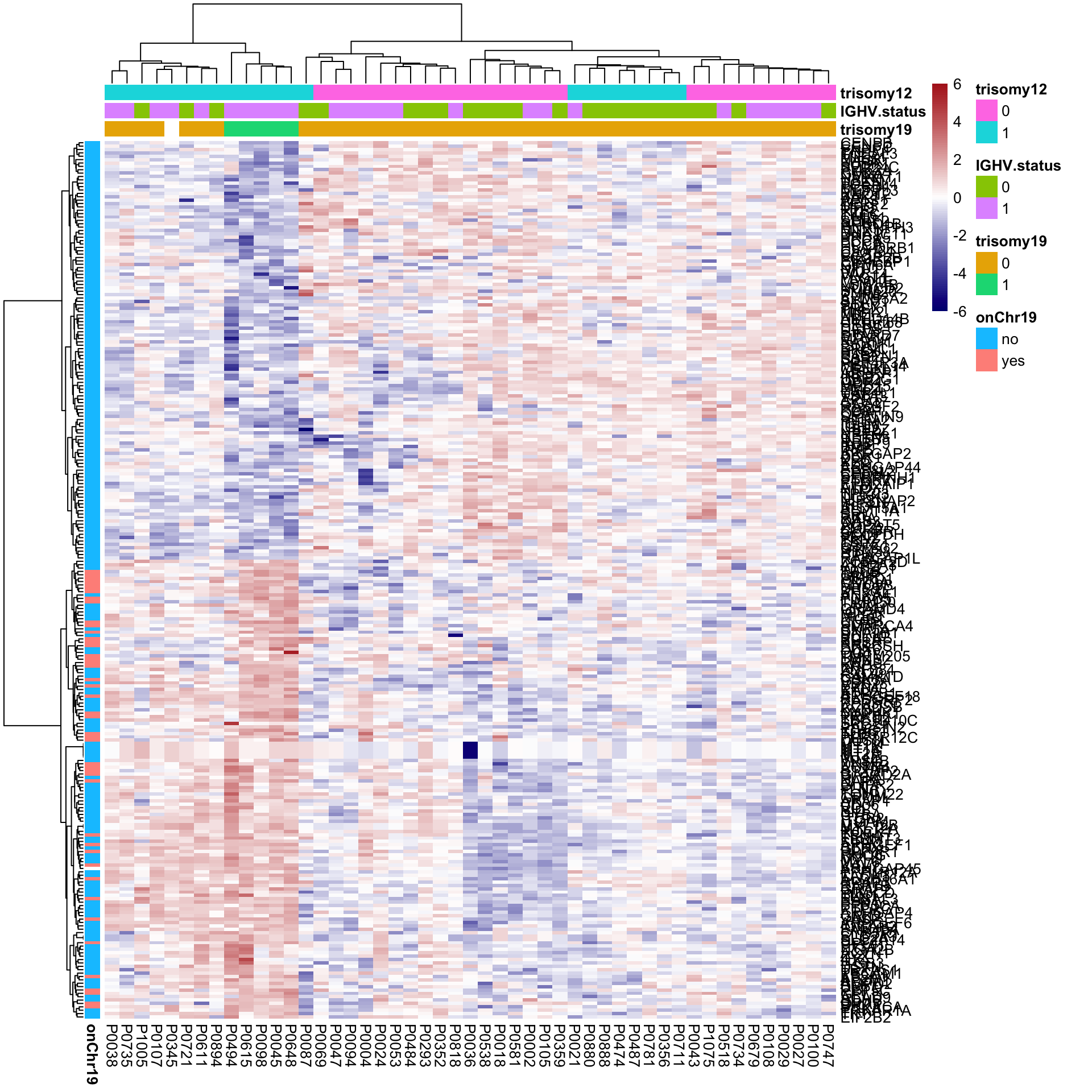
Plot top 9 most differentially expressed proteins
plotTab <- filter(protTab, name %in% corRes.sig$name[1:9]) %>% dplyr::rename(expression = QRILC) %>%
  mutate(trisomy19 = patMeta[match(colID, patMeta$Patient.ID),]$trisomy19) %>%
  filter(!is.na(trisomy19))
ggplot(plotTab, aes(x=trisomy19, y =  expression)) + geom_boxplot(aes(fill = trisomy19)) + geom_point() +
  facet_wrap(~name, scale = "free")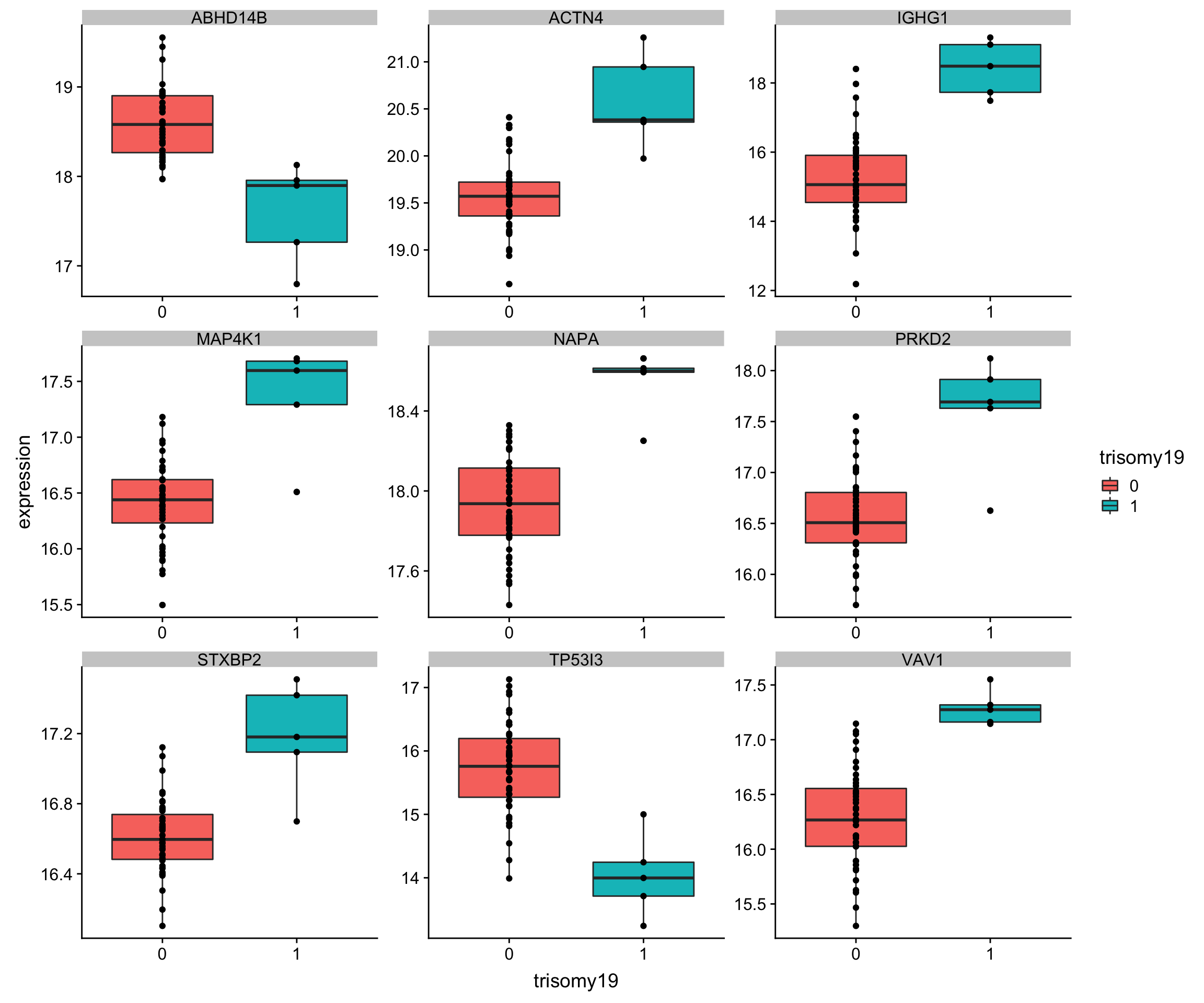
Enrichment analysis
inputTab <- resList %>% filter(P.Value <0.05, Gene == "trisomy19") %>%
  mutate(name = rowData(protCLL[id,])$hgnc_symbol) %>% filter(!is.na(name)) %>%
  distinct(name, .keep_all = TRUE) %>%
  select(name, t) %>% data.frame() %>% column_to_rownames("name")
enRes <- list()
enRes[["HALLMARK"]] <- runGSEA(inputTab, gmts$H, "page")
enRes[["KEGG"]] <- runGSEA(inputTab, gmts$KEGG, "page")
p <- plotEnrichmentBar(enRes, pCut =0.05, ifFDR= FALSE)
Coordinate system already present. Adding new coordinate system, which will replace the existing one.
Coordinate system already present. Adding new coordinate system, which will replace the existing one.#pdf("tri12Enrich.pdf", height = 15, width = 6)
plot(p)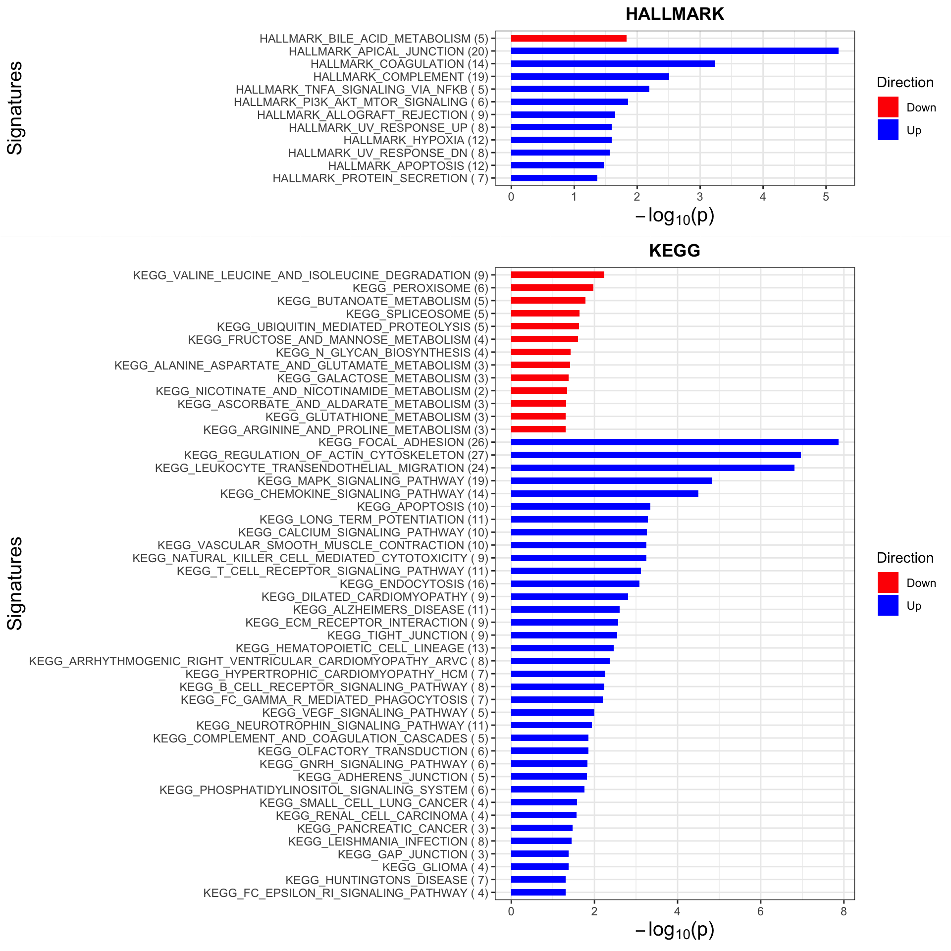
#dev.off()
sessionInfo()R version 3.6.0 (2019-04-26)
Platform: x86_64-apple-darwin15.6.0 (64-bit)
Running under: macOS 10.15.4
Matrix products: default
BLAS: /Library/Frameworks/R.framework/Versions/3.6/Resources/lib/libRblas.0.dylib
LAPACK: /Library/Frameworks/R.framework/Versions/3.6/Resources/lib/libRlapack.dylib
locale:
[1] en_US.UTF-8/en_US.UTF-8/en_US.UTF-8/C/en_US.UTF-8/en_US.UTF-8
attached base packages:
[1] parallel stats4 stats graphics grDevices utils datasets
[8] methods base
other attached packages:
[1] forcats_0.4.0 stringr_1.4.0
[3] dplyr_0.8.5 purrr_0.3.3
[5] readr_1.3.1 tidyr_1.0.0
[7] tibble_3.0.0 tidyverse_1.3.0
[9] SummarizedExperiment_1.14.0 DelayedArray_0.10.0
[11] BiocParallel_1.18.0 matrixStats_0.54.0
[13] Biobase_2.44.0 GenomicRanges_1.36.0
[15] GenomeInfoDb_1.20.0 IRanges_2.18.1
[17] S4Vectors_0.22.0 BiocGenerics_0.30.0
[19] jyluMisc_0.1.5 pheatmap_1.0.12
[21] piano_2.0.2 proDA_1.1.2
[23] cowplot_0.9.4 ggplot2_3.3.0
loaded via a namespace (and not attached):
[1] readxl_1.3.1 backports_1.1.4 fastmatch_1.1-0
[4] drc_3.0-1 workflowr_1.6.0 igraph_1.2.4.1
[7] shinydashboard_0.7.1 splines_3.6.0 crosstalk_1.0.0
[10] TH.data_1.0-10 digest_0.6.19 htmltools_0.4.0
[13] fansi_0.4.0 gdata_2.18.0 magrittr_1.5
[16] cluster_2.1.0 openxlsx_4.1.0.1 limma_3.40.2
[19] modelr_0.1.5 sandwich_2.5-1 colorspace_1.4-1
[22] ggrepel_0.8.1 rvest_0.3.5 haven_2.2.0
[25] xfun_0.8 crayon_1.3.4 RCurl_1.95-4.12
[28] jsonlite_1.6 survival_2.44-1.1 zoo_1.8-6
[31] glue_1.3.2 survminer_0.4.4 gtable_0.3.0
[34] zlibbioc_1.30.0 XVector_0.24.0 car_3.0-3
[37] abind_1.4-5 scales_1.1.0 mvtnorm_1.0-11
[40] DBI_1.0.0 relations_0.6-8 Rcpp_1.0.1
[43] plotrix_3.7-6 xtable_1.8-4 cmprsk_2.2-8
[46] foreign_0.8-71 km.ci_0.5-2 DT_0.7
[49] htmlwidgets_1.3 httr_1.4.1 fgsea_1.10.0
[52] gplots_3.0.1.1 RColorBrewer_1.1-2 ellipsis_0.2.0
[55] farver_2.0.3 pkgconfig_2.0.2 dbplyr_1.4.2
[58] utf8_1.1.4 labeling_0.3 tidyselect_1.0.0
[61] rlang_0.4.5 later_0.8.0 munsell_0.5.0
[64] cellranger_1.1.0 tools_3.6.0 visNetwork_2.0.7
[67] cli_1.1.0 generics_0.0.2 broom_0.5.2
[70] evaluate_0.14 yaml_2.2.0 knitr_1.23
[73] fs_1.4.0 zip_2.0.2 survMisc_0.5.5
[76] caTools_1.17.1.2 nlme_3.1-140 mime_0.7
[79] slam_0.1-45 xml2_1.2.2 rstudioapi_0.10
[82] compiler_3.6.0 curl_3.3 ggsignif_0.5.0
[85] marray_1.62.0 reprex_0.3.0 stringi_1.4.3
[88] lattice_0.20-38 Matrix_1.2-17 shinyjs_1.0
[91] KMsurv_0.1-5 vctrs_0.2.4 pillar_1.4.3
[94] lifecycle_0.2.0 data.table_1.12.2 bitops_1.0-6
[97] httpuv_1.5.1 R6_2.4.0 promises_1.0.1
[100] KernSmooth_2.23-15 gridExtra_2.3 rio_0.5.16
[103] codetools_0.2-16 MASS_7.3-51.4 gtools_3.8.1
[106] exactRankTests_0.8-30 assertthat_0.2.1 rprojroot_1.3-2
[109] withr_2.1.2 multcomp_1.4-10 GenomeInfoDbData_1.2.1
[112] hms_0.5.2 grid_3.6.0 rmarkdown_1.13
[115] carData_3.0-2 git2r_0.26.1 maxstat_0.7-25
[118] ggpubr_0.2.1 sets_1.0-18 shiny_1.3.2
[121] lubridate_1.7.4