Analysis of the correlations between RNA and protein expression
Junyan Lu
2020-06-09
Last updated: 2020-06-17
Checks: 5 2
Knit directory: Proteomics/analysis/
This reproducible R Markdown analysis was created with workflowr (version 1.6.0). The Checks tab describes the reproducibility checks that were applied when the results were created. The Past versions tab lists the development history.
The R Markdown is untracked by Git. To know which version of the R Markdown file created these results, you’ll want to first commit it to the Git repo. If you’re still working on the analysis, you can ignore this warning. When you’re finished, you can run wflow_publish to commit the R Markdown file and build the HTML.
Great job! The global environment was empty. Objects defined in the global environment can affect the analysis in your R Markdown file in unknown ways. For reproduciblity it’s best to always run the code in an empty environment.
The command set.seed(20200227) was run prior to running the code in the R Markdown file. Setting a seed ensures that any results that rely on randomness, e.g. subsampling or permutations, are reproducible.
Great job! Recording the operating system, R version, and package versions is critical for reproducibility.
- unnamed-chunk-18
- unnamed-chunk-24
To ensure reproducibility of the results, delete the cache directory correlateRNAexpression_cache and re-run the analysis. To have workflowr automatically delete the cache directory prior to building the file, set delete_cache = TRUE when running wflow_build() or wflow_publish().
Great job! Using relative paths to the files within your workflowr project makes it easier to run your code on other machines.
Great! You are using Git for version control. Tracking code development and connecting the code version to the results is critical for reproducibility. The version displayed above was the version of the Git repository at the time these results were generated.
Note that you need to be careful to ensure that all relevant files for the analysis have been committed to Git prior to generating the results (you can use wflow_publish or wflow_git_commit). workflowr only checks the R Markdown file, but you know if there are other scripts or data files that it depends on. Below is the status of the Git repository when the results were generated:
Ignored files:
    Ignored:    .DS_Store
    Ignored:    .Rhistory
    Ignored:    .Rproj.user/
    Ignored:    analysis/.DS_Store
    Ignored:    analysis/.Rhistory
    Ignored:    analysis/analysisDrugResponses_IC50_cache/
    Ignored:    analysis/analysisDrugResponses_cache/
    Ignored:    analysis/complexAnalysis_IGHV_alternative_cache/
    Ignored:    analysis/complexAnalysis_IGHV_cache/
    Ignored:    analysis/complexAnalysis_trisomy12_alteredPQR_cache/
    Ignored:    analysis/complexAnalysis_trisomy12_alternative_cache/
    Ignored:    analysis/complexAnalysis_trisomy12_cache/
    Ignored:    analysis/correlateCLLPD_cache/
    Ignored:    analysis/correlateRNAexpression_cache/
    Ignored:    analysis/predictOutcome_cache/
    Ignored:    code/.Rhistory
    Ignored:    data/.DS_Store
    Ignored:    output/.DS_Store

Untracked files:
    Untracked:  analysis/CNVanalysis_11q.Rmd
    Untracked:  analysis/CNVanalysis_trisomy12.Rmd
    Untracked:  analysis/CNVanalysis_trisomy19.Rmd
    Untracked:  analysis/analysisDrugResponses.Rmd
    Untracked:  analysis/analysisDrugResponses_IC50.Rmd
    Untracked:  analysis/analysisPCA.Rmd
    Untracked:  analysis/analysisSplicing.Rmd
    Untracked:  analysis/analysisTrisomy19.Rmd
    Untracked:  analysis/annotateCNV.Rmd
    Untracked:  analysis/complexAnalysis_IGHV.Rmd
    Untracked:  analysis/complexAnalysis_IGHV_alternative.Rmd
    Untracked:  analysis/complexAnalysis_overall.Rmd
    Untracked:  analysis/complexAnalysis_trisomy12.Rmd
    Untracked:  analysis/complexAnalysis_trisomy12_alternative.Rmd
    Untracked:  analysis/correlateGenomic_PC12adjusted.Rmd
    Untracked:  analysis/correlateGenomic_noBlock.Rmd
    Untracked:  analysis/correlateGenomic_noBlock_MCLL.Rmd
    Untracked:  analysis/correlateGenomic_noBlock_UCLL.Rmd
    Untracked:  analysis/correlateRNAexpression.Rmd
    Untracked:  analysis/default.css
    Untracked:  analysis/del11q.pdf
    Untracked:  analysis/del11q_norm.pdf
    Untracked:  analysis/peptideValidate.Rmd
    Untracked:  analysis/plotExpressionCNV.Rmd
    Untracked:  analysis/processPeptides_LUMOS.Rmd
    Untracked:  analysis/style.css
    Untracked:  analysis/trisomy12.pdf
    Untracked:  analysis/trisomy12_AFcor.Rmd
    Untracked:  analysis/trisomy12_norm.pdf
    Untracked:  code/AlteredPQR.R
    Untracked:  code/utils.R
    Untracked:  data/190909_CLL_prot_abund_med_norm.tsv
    Untracked:  data/190909_CLL_prot_abund_no_norm.tsv
    Untracked:  data/20190423_Proteom_submitted_samples_bereinigt.xlsx
    Untracked:  data/20191025_Proteom_submitted_samples_final.xlsx
    Untracked:  data/LUMOS/
    Untracked:  data/LUMOS_peptides/
    Untracked:  data/LUMOS_protAnnotation.csv
    Untracked:  data/LUMOS_protAnnotation_fix.csv
    Untracked:  data/SampleAnnotation_cleaned.xlsx
    Untracked:  data/example_proteomics_data
    Untracked:  data/facTab_IC50atLeast3New.RData
    Untracked:  data/gmts/
    Untracked:  data/mapEnsemble.txt
    Untracked:  data/mapSymbol.txt
    Untracked:  data/proteins_in_complexes
    Untracked:  data/pyprophet_export_aligned.csv
    Untracked:  data/timsTOF_protAnnotation.csv
    Untracked:  output/LUMOS_processed.RData
    Untracked:  output/cnv_plots.zip
    Untracked:  output/cnv_plots/
    Untracked:  output/cnv_plots_norm.zip
    Untracked:  output/dxdCLL.RData
    Untracked:  output/exprCNV.RData
    Untracked:  output/lassoResults_CPS.RData
    Untracked:  output/lassoResults_IC50.RData
    Untracked:  output/pepCLL_lumos.RData
    Untracked:  output/pepTab_lumos.RData
    Untracked:  output/plotCNV_allChr11_diff.pdf
    Untracked:  output/plotCNV_del11q_sum.pdf
    Untracked:  output/proteomic_LUMOS_20200227.RData
    Untracked:  output/proteomic_LUMOS_20200320.RData
    Untracked:  output/proteomic_LUMOS_20200430.RData
    Untracked:  output/proteomic_timsTOF_20200227.RData
    Untracked:  output/splicingResults.RData
    Untracked:  output/timsTOF_processed.RData
    Untracked:  plotCNV_del11q_diff.pdf

Unstaged changes:
    Modified:   analysis/_site.yml
    Modified:   analysis/analysisSF3B1.Rmd
    Modified:   analysis/compareProteomicsRNAseq.Rmd
    Modified:   analysis/correlateCLLPD.Rmd
    Modified:   analysis/correlateGenomic.Rmd
    Deleted:    analysis/correlateGenomic_removePC.Rmd
    Modified:   analysis/correlateMIR.Rmd
    Modified:   analysis/correlateMethylationCluster.Rmd
    Modified:   analysis/index.Rmd
    Modified:   analysis/predictOutcome.Rmd
    Modified:   analysis/processProteomics_LUMOS.Rmd
    Modified:   analysis/qualityControl_LUMOS.Rmd
Note that any generated files, e.g. HTML, png, CSS, etc., are not included in this status report because it is ok for generated content to have uncommitted changes.
There are no past versions. Publish this analysis with wflow_publish() to start tracking its development.
Overall associations
Process both datasets
colnames(dds) <- dds$PatID
dds <- estimateSizeFactors(dds)
sampleOverlap <- intersect(colnames(protCLL), colnames(dds))
geneOverlap <- intersect(rowData(protCLL)$ensembl_gene_id, rownames(dds))
ddsSub <- dds[geneOverlap, sampleOverlap]
protSub <- protCLL[match(geneOverlap, rowData(protCLL)$ensembl_gene_id), sampleOverlap]

#how many gene don't have RNA expression at all?
noExp <- rowSums(counts(ddsSub)) == 0

#remove those genes in both datasets
ddsSub <- ddsSub[!noExp,]
protSub <- protSub[!noExp,]

#remove proteins with duplicated identifiers
protSub <- protSub[!duplicated(rowData(protSub)$name)]

geneOverlap <- intersect(rowData(protSub)$ensembl_gene_id, rownames(ddsSub))

ddsSub.vst <- varianceStabilizingTransformation(ddsSub)
Calculate correlations between protein abundance and RNA expression
rnaMat <- assay(ddsSub.vst)
proMat <- assays(protSub)[["count"]]
rownames(proMat) <- rowData(protSub)$ensembl_gene_id

corTab <- lapply(geneOverlap, function(n) {
  rna <- rnaMat[n,]
  pro.raw <- proMat[n,]
  res.raw <- cor.test(rna, pro.raw, use = "pairwise.complete.obs")
  tibble(id = n,
         p = res.raw$p.value,
         coef = res.raw$estimate)
}) %>% bind_rows() %>%
  arrange(desc(coef)) %>% mutate(p.adj = p.adjust(p, method = "BH"),
                                 symbol = rowData(dds[id,])$symbol,
                                 chr = rowData(dds[id,])$chromosome)
Plot the distribution of correlation coefficient
ggplot(corTab, aes(x=coef)) + geom_histogram(position = "identity", col = "grey50", alpha =0.3, bins =100) +
geom_vline(xintercept = 0, col = "red", linetype = "dashed") +
xlab("Pearson's correlation coefficient") 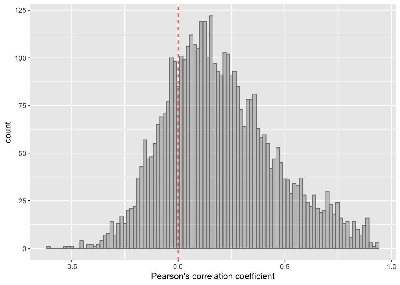 Most of the correlations are positive, which is reasonable.
ggplot(filter(corTab,!is.na(chr)), aes(x=coef)) + geom_histogram(position = "identity", col = "grey50", alpha =0.3, bins =100) +
geom_vline(xintercept = 0, col = "red", linetype = "dashed") + facet_wrap(~chr,ncol=3) +
xlab("Pearson's correlation coefficient") 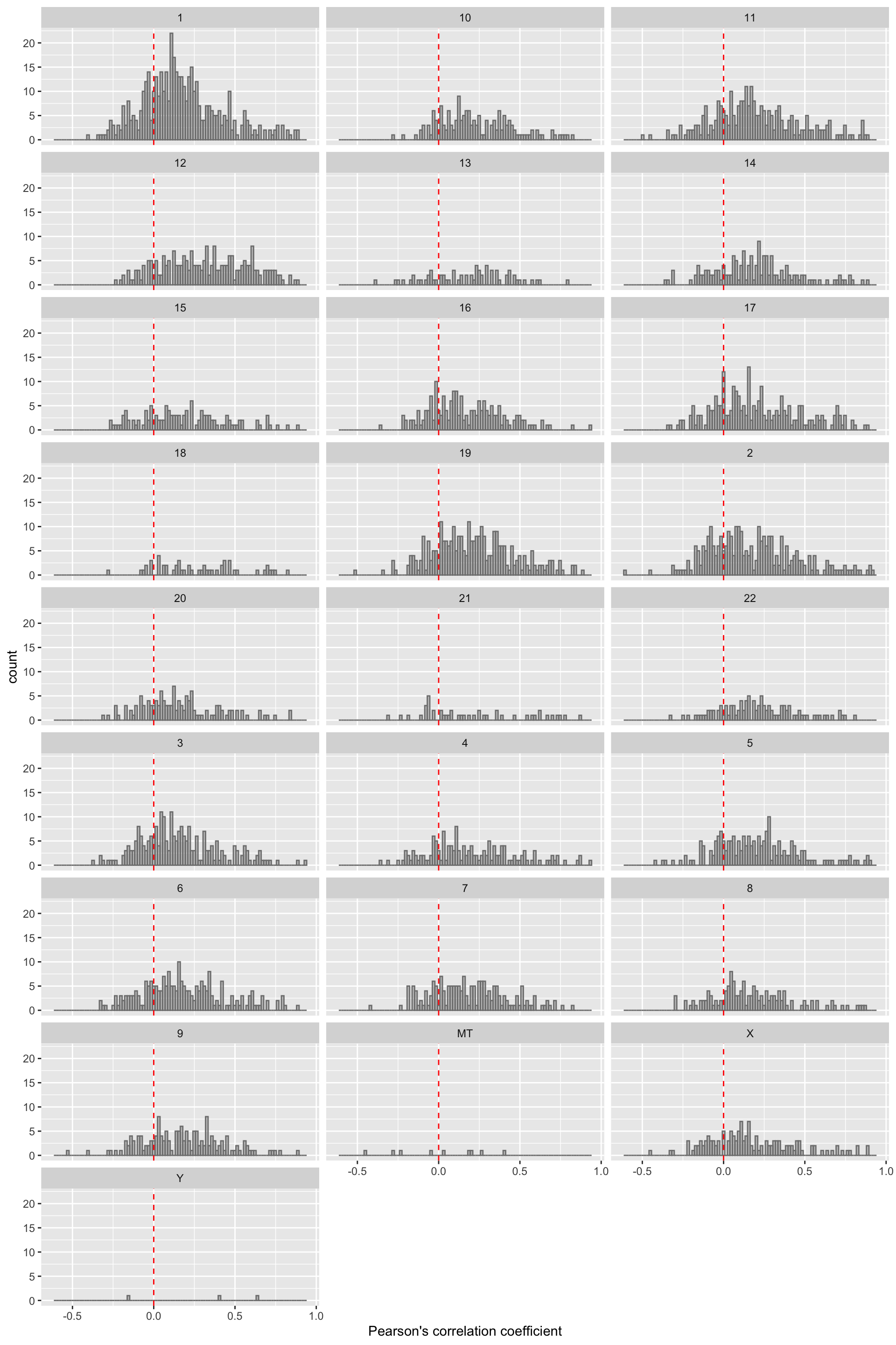 Similar trend can be observed for each chromosome.
Correlation between protein/rna abundance and protein-RNA correltions
protMean <- rowMeans(assays(protSub)[["count"]],na.rm = TRUE)
names(protMean) <- rowData(protSub)$ensembl_gene_id
rnaMean <- rowMeans(counts(ddsSub, normalized = TRUE),na.rm=TRUE)
corTab <- mutate(corTab, meanProt = protMean[id], meanRNA=rnaMean[id])
Protein abundance VS correlation
ggplot(corTab, aes(x=meanProt, y = coef)) + geom_point() + geom_smooth(method= "lm") +
  xlab("Mean protein abundance") + ylab("Correlation coefficient")
cor.test(corTab$meanProt, corTab$coef)
    Pearson's product-moment correlation

data:  corTab$meanProt and corTab$coef
t = -0.57856, df = 4231, p-value = 0.5629
alternative hypothesis: true correlation is not equal to 0
95 percent confidence interval:
 -0.03901014  0.02123779
sample estimates:
         cor
-0.008894243
No correlation.
RNA abundance VS correlation
ggplot(corTab, aes(x=meanRNA, y = coef)) + geom_point() + geom_smooth(method= "lm") +
  xlab("Mean RNA abundance") + ylab("Correlation coefficient") + scale_x_log10()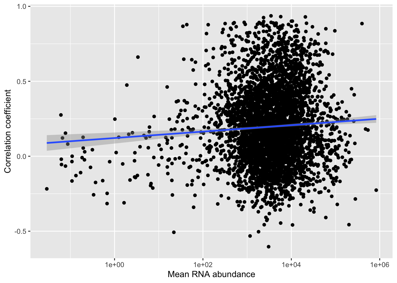
cor.test(corTab$coef, corTab$meanRNA)
    Pearson's product-moment correlation

data:  corTab$coef and corTab$meanRNA
t = -1.3185, df = 4231, p-value = 0.1874
alternative hypothesis: true correlation is not equal to 0
95 percent confidence interval:
 -0.050361859  0.009866109
sample estimates:
        cor
-0.02026626
No correlation.
For proteins in complex and not in complex
int_pairs = read.table ("../data/proteins_in_complexes", sep = "\t", stringsAsFactors = FALSE, header = T)

sourceTab <- int_pairs %>% mutate(Reactome = grepl("Reactome",Evidence_supporting_the_interaction),
         Corum = grepl("Corum",Evidence_supporting_the_interaction)) %>%
  filter(ProtA %in% rownames(protSub) & ProtB %in% rownames(protSub)) %>%
  mutate(database = case_when(
    Reactome & Corum ~ 5,
    Reactome & !Corum ~ 1,
    !Reactome & Corum ~ 2,
    TRUE ~ 0
  )) %>% dplyr::select(ProtA, ProtB, database) %>% gather(key = "prot", value = "id", -database) %>%
  distinct(database, id) %>%
  group_by(id) %>% summarise(n=sum(database)) %>%
  mutate(database = case_when(
    n ==0 ~ "other",
    n ==1 ~ "Reactome",
    n ==2 ~ "Corum",
    n >= 3 ~ "both"
  )) %>%
  mutate(id = rowData(protCLL)$ensembl_gene_id[match(id, rownames(protCLL))])

comProt <- unique(c(int_pairs$ProtA, int_pairs$ProtB))
comGene <- rowData(protCLL)$ensembl_gene_id[match(comProt, rownames(protCLL))]
comGene <- na.omit(comGene)
corTab <- corTab %>% mutate(inComplex = ifelse(id %in% comGene, "yes","no")) %>%
mutate(database = sourceTab[match(id, sourceTab$id),]$database)
ggplot(corTab, aes(x=coef, fill = inComplex, y=..density..)) + geom_histogram(position = "identity", col = "grey50", alpha =0.3, bins =100) +
geom_vline(xintercept = 0, col = "red", linetype = "dashed") +
xlab("Pearson's correlation coefficient") 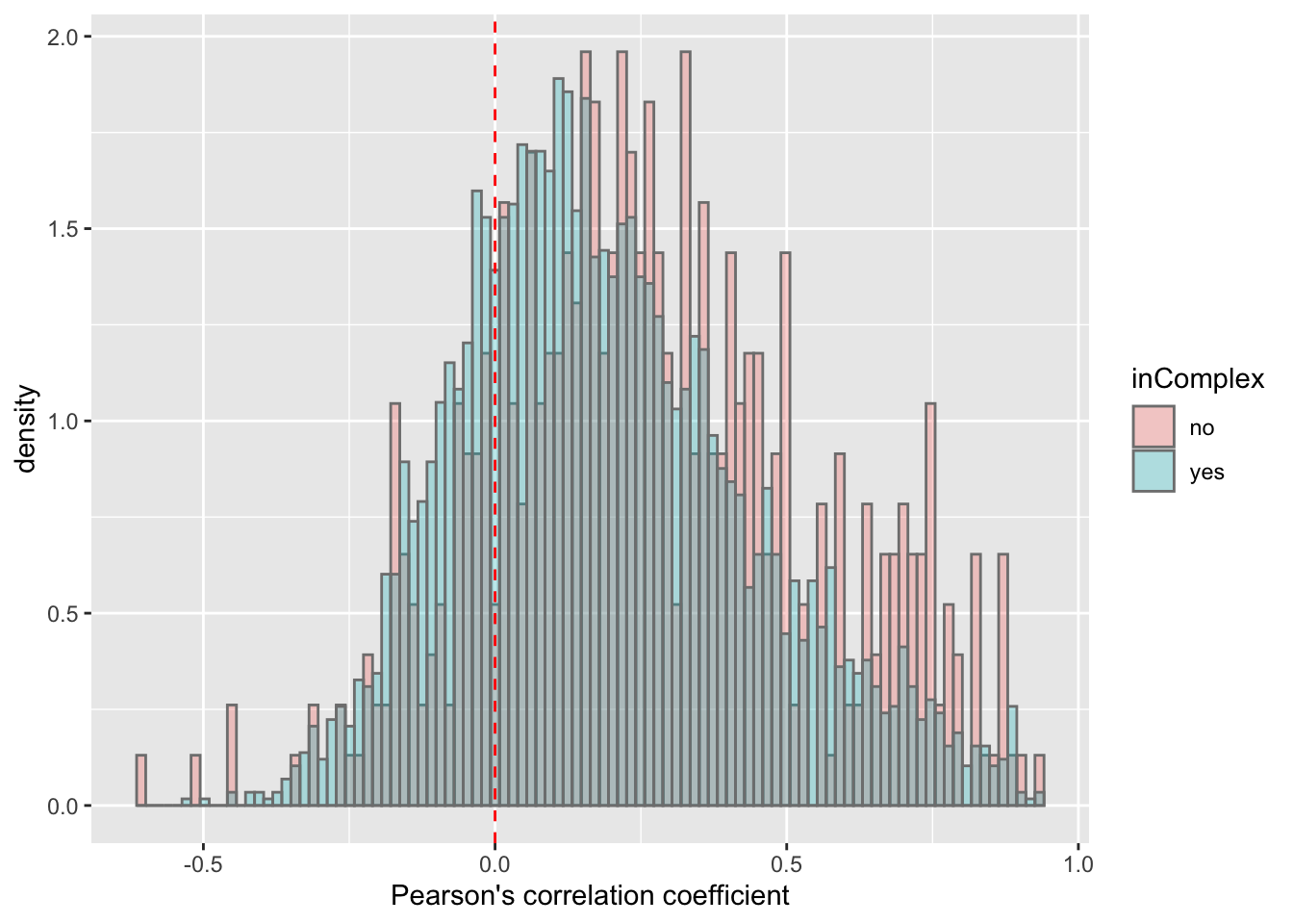 There’s a slight trend that proteins not in complex tend to have higher protein-RNA expression correlations, which is reasonable, as proteins form complexes may be more regulated by buffering effect.
T-test
t.test(coef~inComplex, corTab, var.equal = TRUE )
    Two Sample t-test

data:  coef by inComplex
t = 6.6141, df = 4231, p-value = 4.204e-11
alternative hypothesis: true difference in means is not equal to 0
95 percent confidence interval:
 0.05679841 0.10465599
sample estimates:
 mean in group no mean in group yes
        0.2683433         0.1876161
ggplot(corTab, aes(x=inComplex, y = coef))+geom_boxplot(aes(fill = inComplex)) + geom_point() +
theme_bw()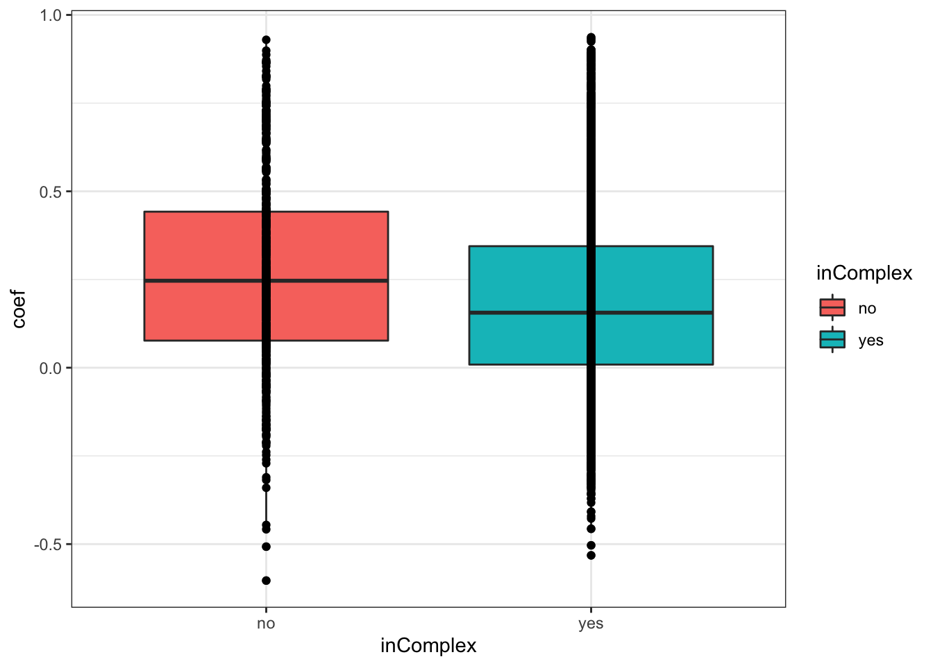
pList <- lapply(na.omit(unique(corTab$database)), function(n) {
plotTab <- filter(corTab, database %in% c(n,NA)) %>%
mutate(database = ifelse(is.na(database),"none",database)) %>%
mutate(database = factor(database, levels = c("none",n)))
p1 <- ggplot(plotTab, aes(x=coef, fill = database, y=..density..)) +
geom_histogram(position = "identity", col = "grey50", alpha =0.3, bins =100) +
geom_vline(xintercept = 0, col = "red", linetype = "dashed") +
xlab("Pearson's correlation coefficient")
p2 <- ggplot(plotTab, aes(x=database, fill = database, y=coef)) +
geom_boxplot() + geom_point() +
ylab("Pearson's correlation coefficient")
cowplot::plot_grid(p1,p2)
})
cowplot::plot_grid(plotlist = pList, ncol=1)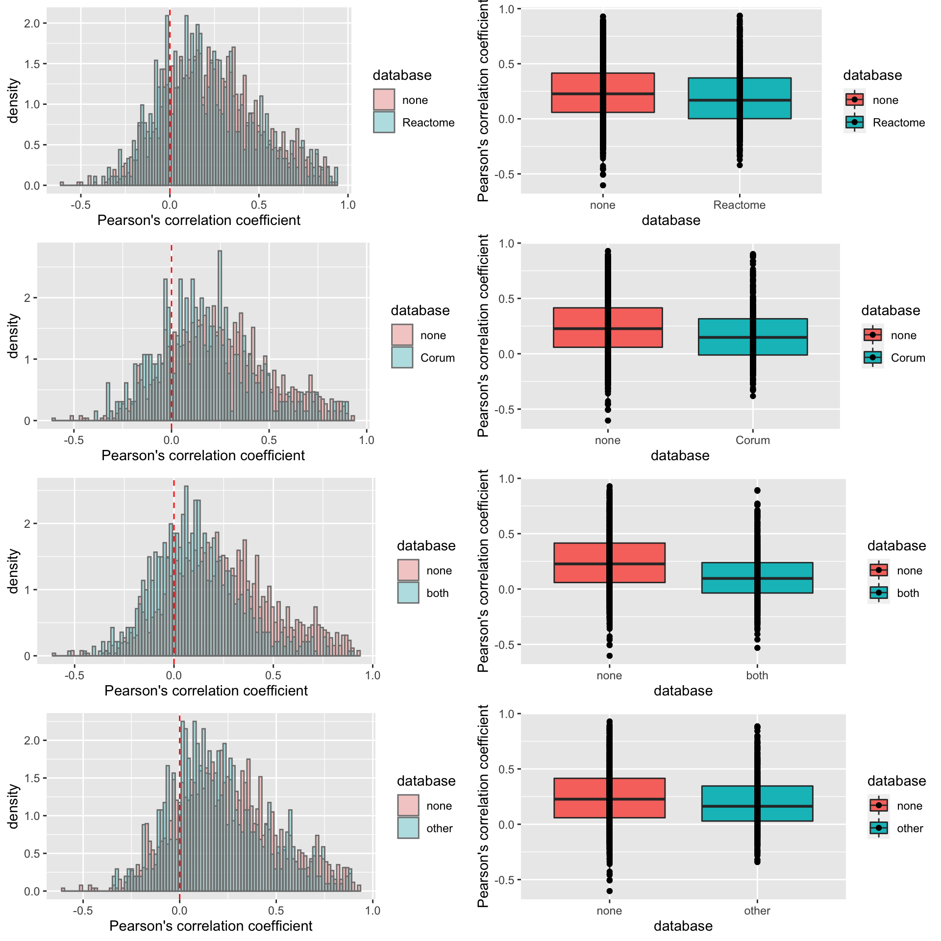 **It seems the difference of correlations coefficient between proteins in complex and not in complex is stronger if we use more stringent criteria for proteins in complexes (annotated as in complexes by both Corum and reactome).
Per chromosome
ggplot(filter(corTab,!is.na(chr)), aes(x=coef,y=..density.., fill =inComplex)) + geom_histogram(position = "identity", col = "grey50", alpha =0.3, bins =100) +
  geom_vline(xintercept = 0, col = "red", linetype = "dashed") + facet_wrap(~chr,ncol=3) +
xlab("Pearson's correlation coefficient") 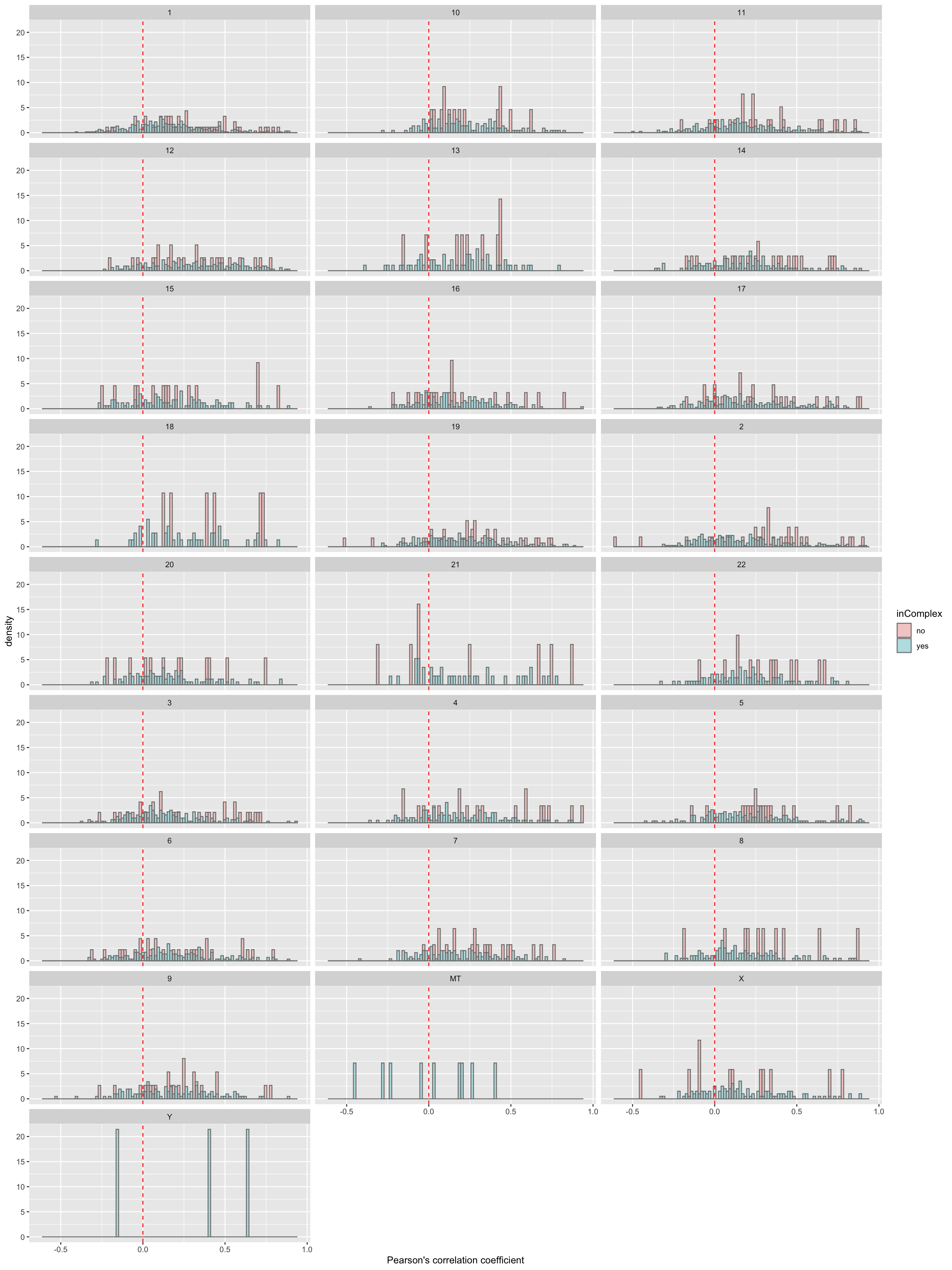
For proteins on chr12
plotTab <- filter(corTab, chr == "12")
ggplot(plotTab, aes(x=coef,y=..density.., fill =inComplex)) +
geom_histogram(position = "identity", col = "grey50", alpha =0.3, bins =100) +
geom_vline(xintercept = 0, col = "red", linetype = "dashed") +
xlab("Pearson's correlation coefficient") 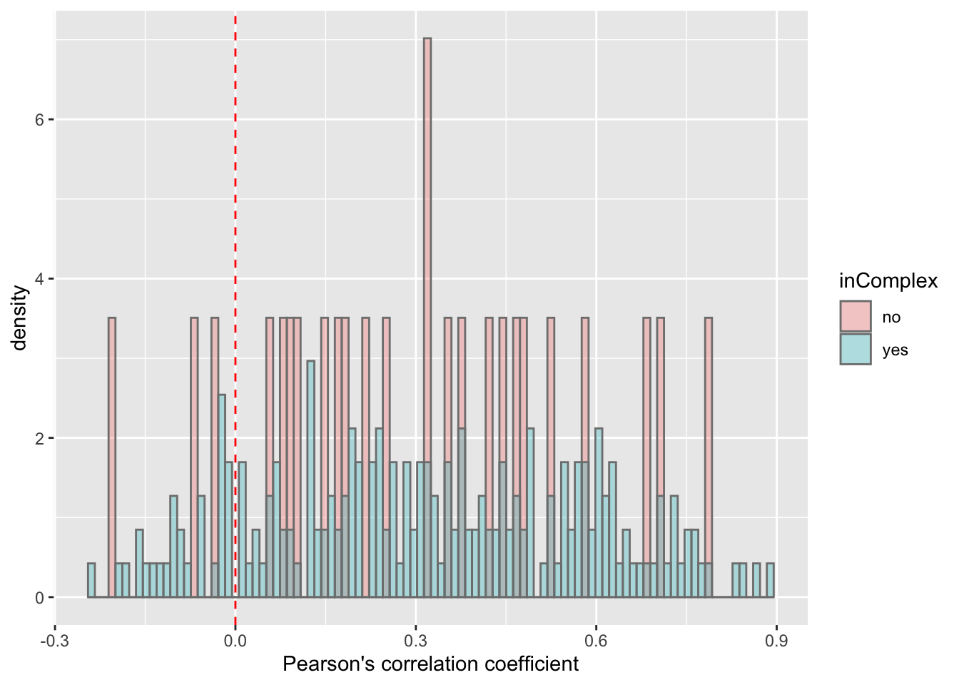 T-test
t.test(coef~inComplex, plotTab, var.equal = TRUE )
    Two Sample t-test

data:  coef by inComplex
t = -0.38296, df = 230, p-value = 0.7021
alternative hypothesis: true difference in means is not equal to 0
95 percent confidence interval:
 -0.13065038  0.08812787
sample estimates:
 mean in group no mean in group yes
        0.2989923         0.3202535
ggplot(plotTab, aes(x=inComplex, y = coef))+geom_boxplot(aes(fill = inComplex)) + geom_point() +
theme_bw()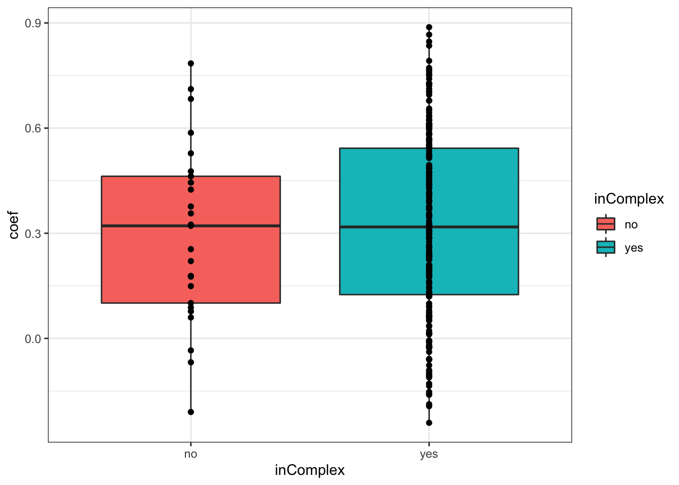
For proteins on chr19
plotTab <- filter(corTab, chr == "19")
ggplot(plotTab, aes(x=coef,y=..density.., fill =inComplex)) +
geom_histogram(position = "identity", col = "grey50", alpha =0.3, bins =100) +
geom_vline(xintercept = 0, col = "red", linetype = "dashed") +
xlab("Pearson's correlation coefficient") 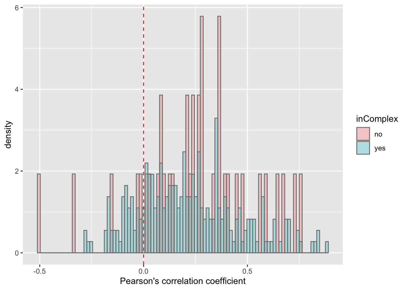
T-test
t.test(coef~inComplex, plotTab, var.equal = TRUE )
Two Sample t-test
data: coef by inComplex
t = 0.78609, df = 295, p-value = 0.4324
alternative hypothesis: true difference in means is not equal to 0
95 percent confidence interval:
-0.05126735 0.11946102
sample estimates:
mean in group no mean in group yes
0.2485261 0.2144293 ggplot(plotTab, aes(x=inComplex, y = coef))+geom_boxplot(aes(fill = inComplex)) + geom_point() +
theme_bw()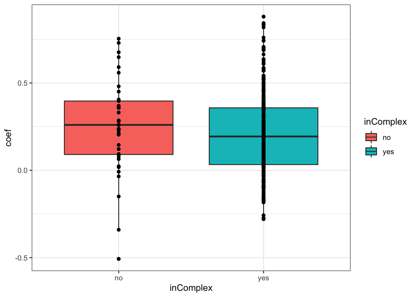
RNA-protein correlation for proteins regulated by trisomy12 or trisomy19
In this part, I want to answer the questions:
1. Whether proteins regulated by trisomy12/trisomy19 (differentially expressed) show a different trend of protein-RNA correlation than other proteins?
2. Whether this difference is related to complex forming?
Trisomy12
Identify proteins regulated by trisomy12 (10% FDR)
protCLL$trisomy12 <- patMeta[match(colnames(protCLL),patMeta$Patient.ID),]$trisomy12
protMat <- assays(protCLL)[["count"]] #without imputation
designMat <- colData(protCLL)[,c("IGHV.status","trisomy12")]
fit <- proDA(protMat, design = ~ .,
col_data = designMat)
resTab.tri12 <- test_diff(fit, "trisomy121") %>%
filter(adj_pval < 0.1) %>%
mutate(symbol = rowData(protCLL[name,])$hgnc_symbol)
dim(resTab.tri12)[1] 1165 11Protien-RNA correlation for proteins associated or not associated with trisomy12
plotTab <- corTab %>% mutate(tri12Regulated = ifelse(symbol %in% resTab.tri12$symbol,"tri12 regulated","not regulated"))
ggplot(plotTab, aes(x=coef,y=..density.., fill =tri12Regulated)) +
geom_histogram(position = "identity", col = "grey50", alpha =0.3, bins =100) +
geom_vline(xintercept = 0, col = "red", linetype = "dashed") +
xlab("Pearson's correlation coefficient") 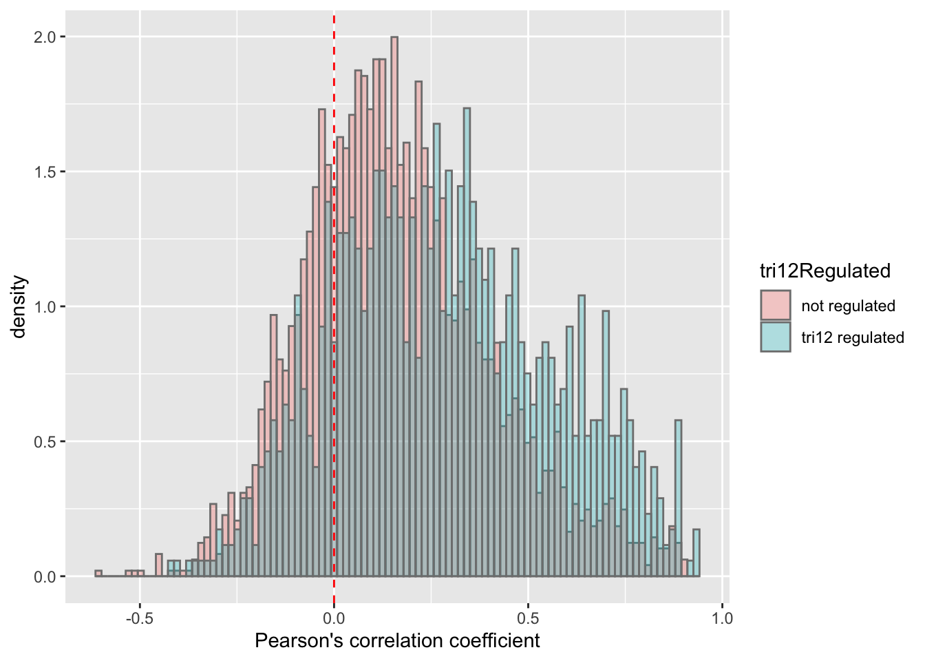
t.test(coef~tri12Regulated, plotTab, var.equal = TRUE )
Two Sample t-test
data: coef by tri12Regulated
t = -13.747, df = 4231, p-value < 2.2e-16
alternative hypothesis: true difference in means is not equal to 0
95 percent confidence interval:
-0.1373007 -0.1030261
sample estimates:
mean in group not regulated mean in group tri12 regulated
0.1654323 0.2855957 ggplot(plotTab, aes(x=tri12Regulated, y = coef))+geom_boxplot(aes(fill = tri12Regulated)) + geom_point() +
theme_bw()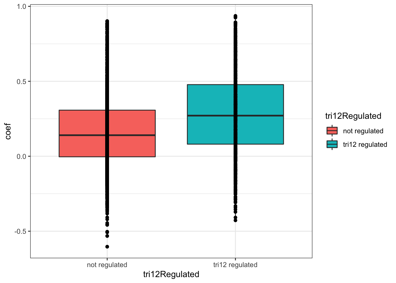 There’s a clear trend that proteins associated with trisomy12 have higher protein-RNA correlation. Maybe a sign of less buffering effect?
Whether complex formation affect this difference?
ggplot(plotTab, aes(x=coef,y=..density.., fill =inComplex)) +
geom_histogram(position = "identity", col = "grey50", alpha =0.3, bins =100) +
geom_vline(xintercept = 0, col = "red", linetype = "dashed") +
xlab("Pearson's correlation coefficient") + facet_wrap(~tri12Regulated)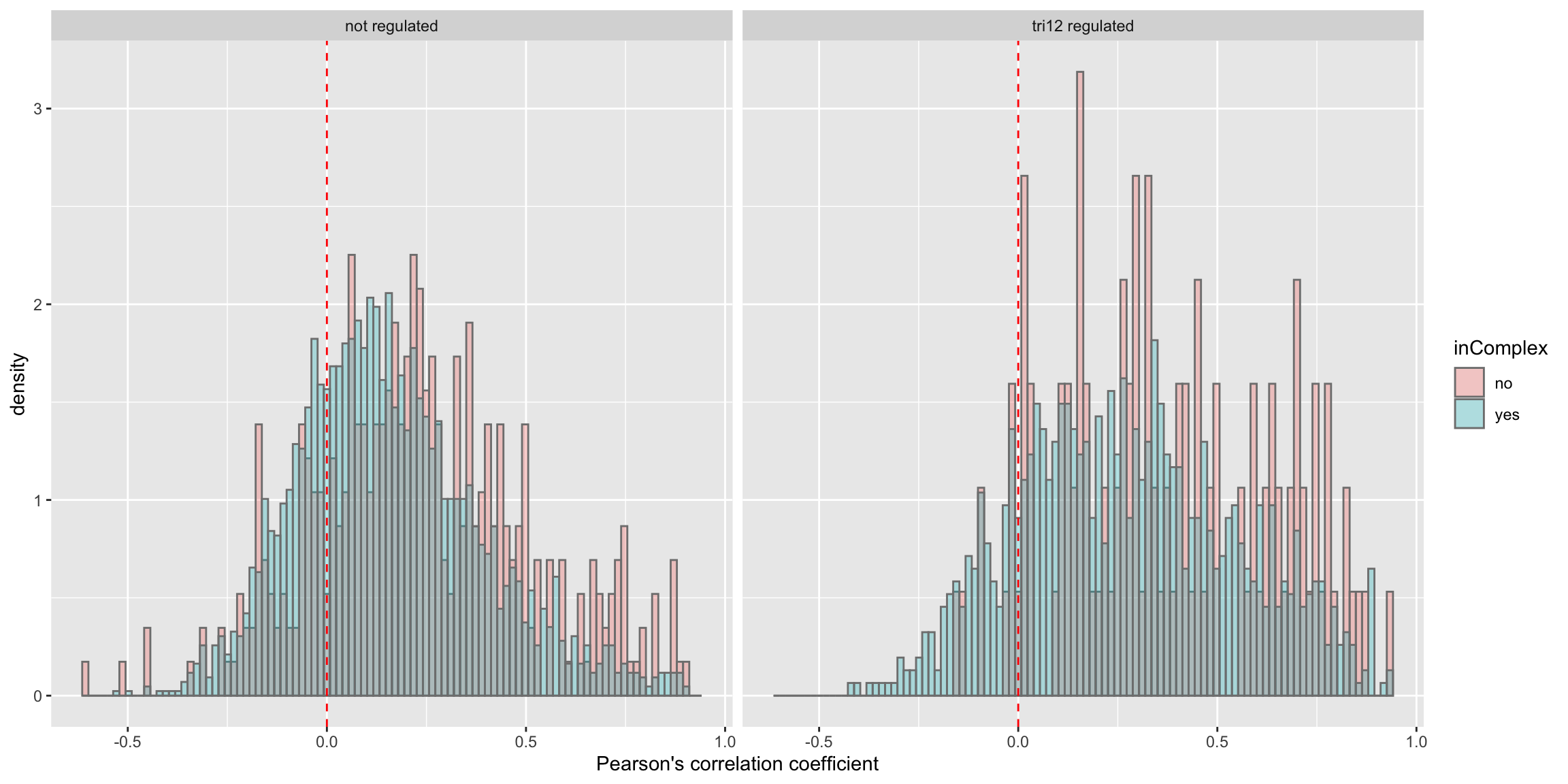
Stratified by trisomy12 regulation
ggplot(plotTab, aes(x=inComplex, y = coef))+geom_boxplot(aes(fill = inComplex)) + geom_point() +
theme_bw() + facet_wrap(~tri12Regulated)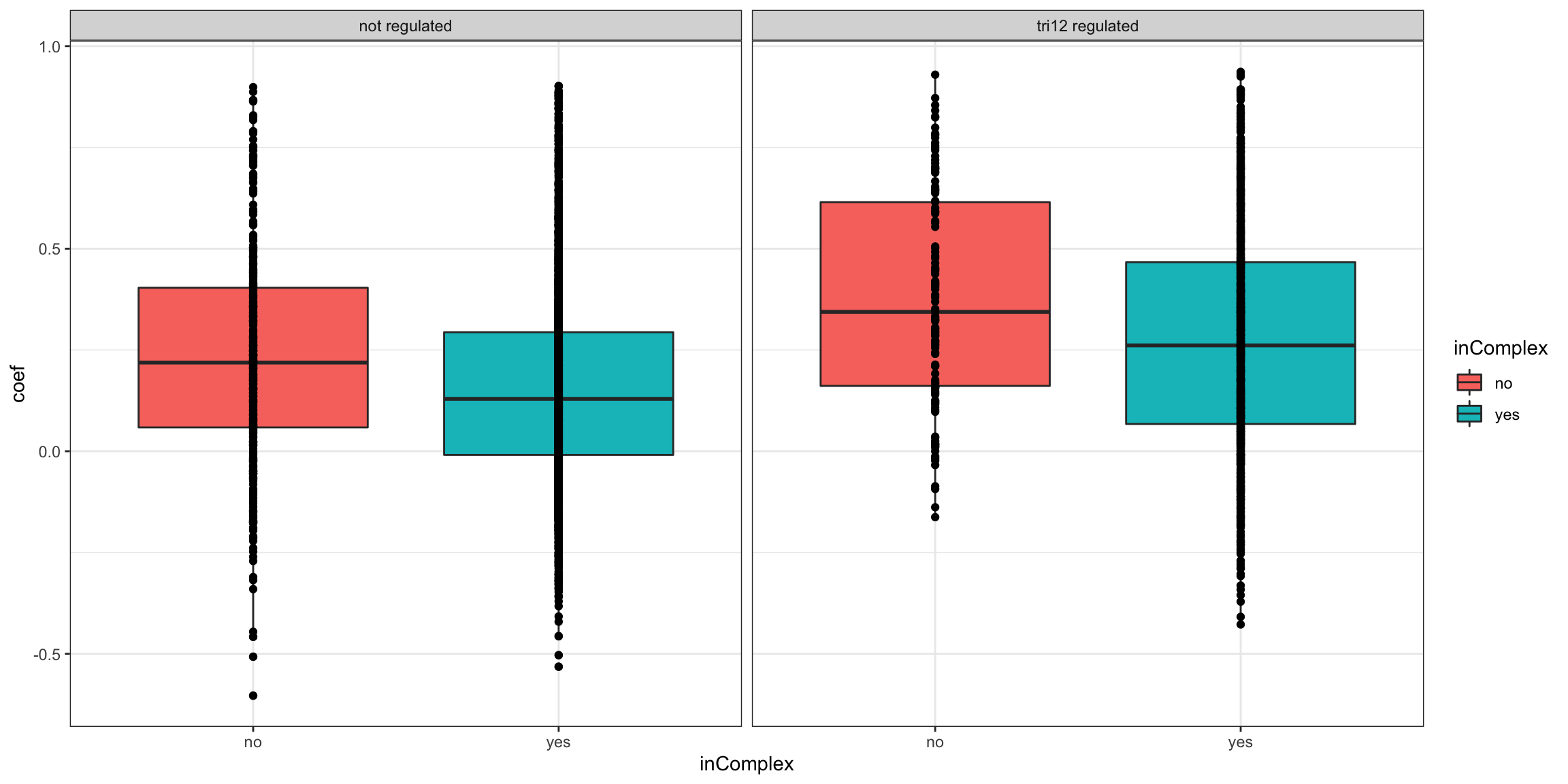
Stratified by complex formation
ggplot(plotTab, aes(x=tri12Regulated, y = coef))+geom_boxplot(aes(fill = tri12Regulated)) + geom_point() +
theme_bw() + facet_wrap(~inComplex)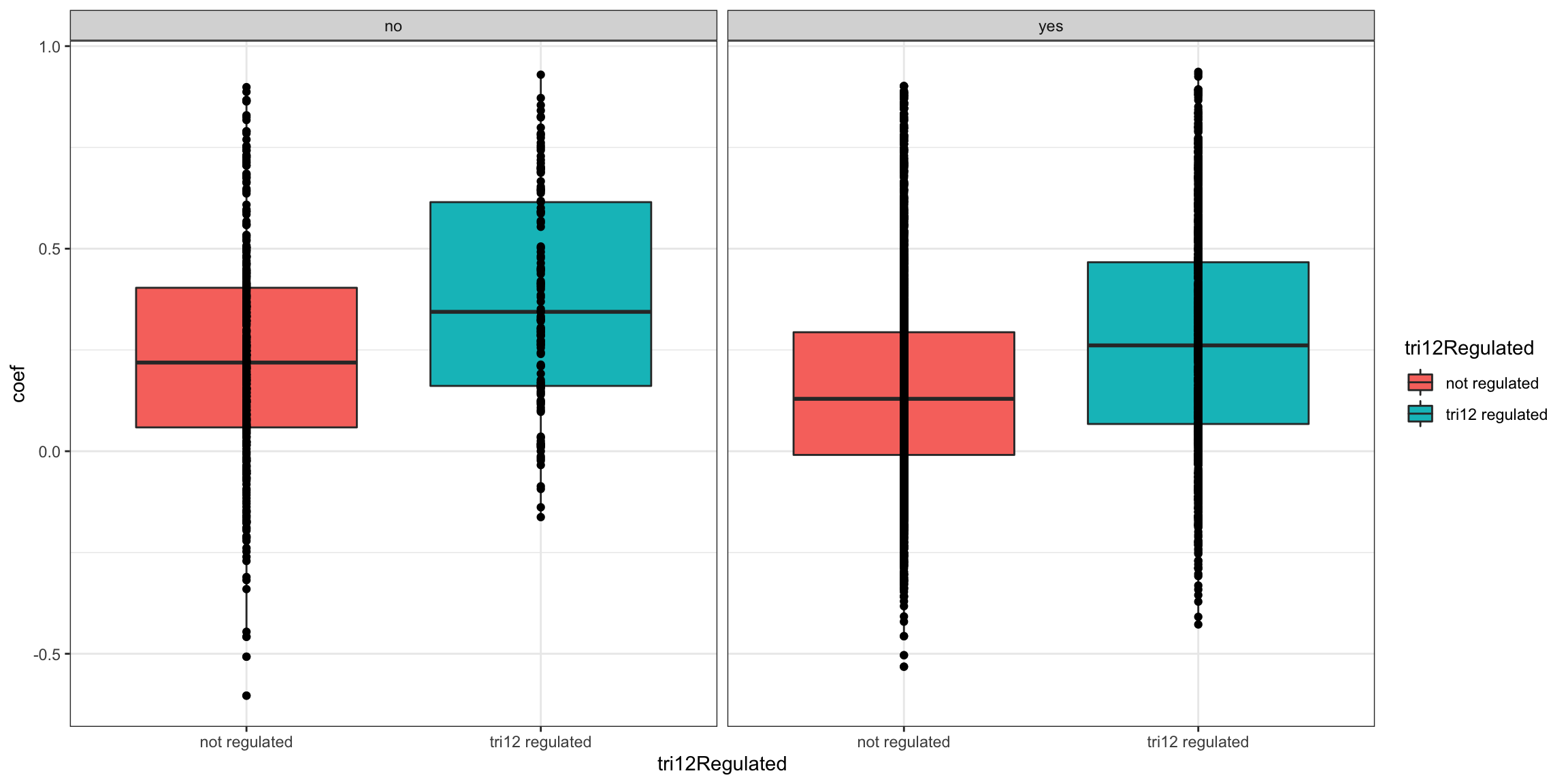
summary(lm(coef~ 1+ tri12Regulated+inComplex, plotTab))
Call:
lm(formula = coef ~ 1 + tri12Regulated + inComplex, data = plotTab)
Residuals:
Min 1Q Median 3Q Max
-0.84202 -0.17669 -0.02234 0.15400 0.74595
Coefficients:
Estimate Std. Error t value Pr(>|t|)
(Intercept) 0.238586 0.011423 20.886 < 2e-16 ***
tri12Regulatedtri12 regulated 0.120999 0.008694 13.918 < 2e-16 ***
inComplexyes -0.083022 0.011938 -6.955 4.08e-12 ***
---
Signif. codes: 0 '***' 0.001 '**' 0.01 '*' 0.05 '.' 0.1 ' ' 1
Residual standard error: 0.2489 on 4230 degrees of freedom
Multiple R-squared: 0.05358, Adjusted R-squared: 0.05313
F-statistic: 119.7 on 2 and 4230 DF, p-value: < 2.2e-16It seems both trisomy12 regulation and complex formation contribute to the variance of RNA-protein correlation independently.
Trisomy19
Identify proteins regulated by trisomy19
(Here I use raw P value < 0.05, otherwise there will be no significant results)
protCLL$trisomy19 <- patMeta[match(colnames(protCLL),patMeta$Patient.ID),]$trisomy19
protSub <- protCLL[,protCLL$IGHV.status %in% "M" & protCLL$trisomy12 %in% 1 &!is.na(protCLL$trisomy19)]
protMat <- assays(protSub)[["count"]] #without imputation
designMat <- colData(protSub)[,c("trisomy19"),drop=FALSE]
fit <- proDA(protMat, design = ~ .,
col_data = designMat)
resTab.tri19 <- test_diff(fit, "trisomy191") %>%
filter(pval < 0.05) %>%
mutate(symbol = rowData(protCLL[name,])$hgnc_symbol)
dim(resTab.tri19)[1] 244 11Protien-RNA correlation for proteins associated or not associated with trisomy19
plotTab <- corTab %>% mutate(tri19Regulated = ifelse(symbol %in% resTab.tri19$symbol,"tri19 regulated","not regulated"))
ggplot(plotTab, aes(x=coef,y=..density.., fill =tri19Regulated)) +
geom_histogram(position = "identity", col = "grey50", alpha =0.3, bins =100) +
geom_vline(xintercept = 0, col = "red", linetype = "dashed") +
xlab("Pearson's correlation coefficient") 
t.test(coef~tri19Regulated, plotTab, var.equal = TRUE )
Two Sample t-test
data: coef by tri19Regulated
t = -9.6542, df = 4231, p-value < 2.2e-16
alternative hypothesis: true difference in means is not equal to 0
95 percent confidence interval:
-0.1996974 -0.1322812
sample estimates:
mean in group not regulated mean in group tri19 regulated
0.1880192 0.3540085 ggplot(plotTab, aes(x=tri19Regulated, y = coef))+geom_boxplot(aes(fill = tri19Regulated)) + geom_point() +
theme_bw() There’s also a clear trend that proteins associated with trisomy19 have higher protein-RNA correlation.
Whether complex formation affect this difference?
ggplot(plotTab, aes(x=coef,y=..density.., fill =inComplex)) +
geom_histogram(position = "identity", col = "grey50", alpha =0.3, bins =100) +
geom_vline(xintercept = 0, col = "red", linetype = "dashed") +
xlab("Pearson's correlation coefficient") + facet_wrap(~tri19Regulated)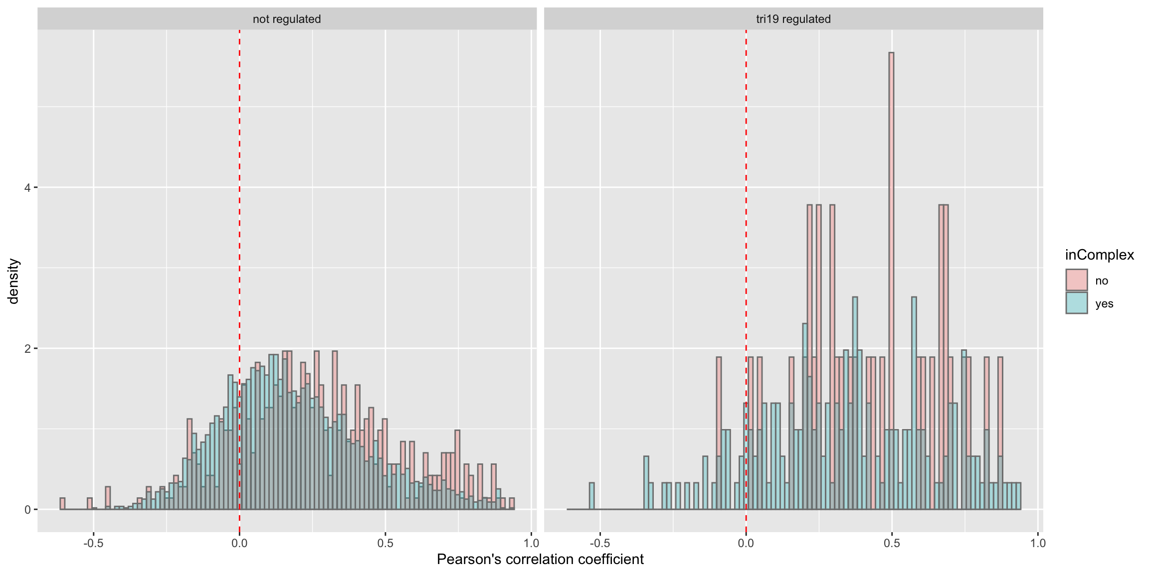
Stratified by trisomy12 regulation
ggplot(plotTab, aes(x=inComplex, y = coef))+geom_boxplot(aes(fill = inComplex)) + geom_point() +
theme_bw() + facet_wrap(~tri19Regulated)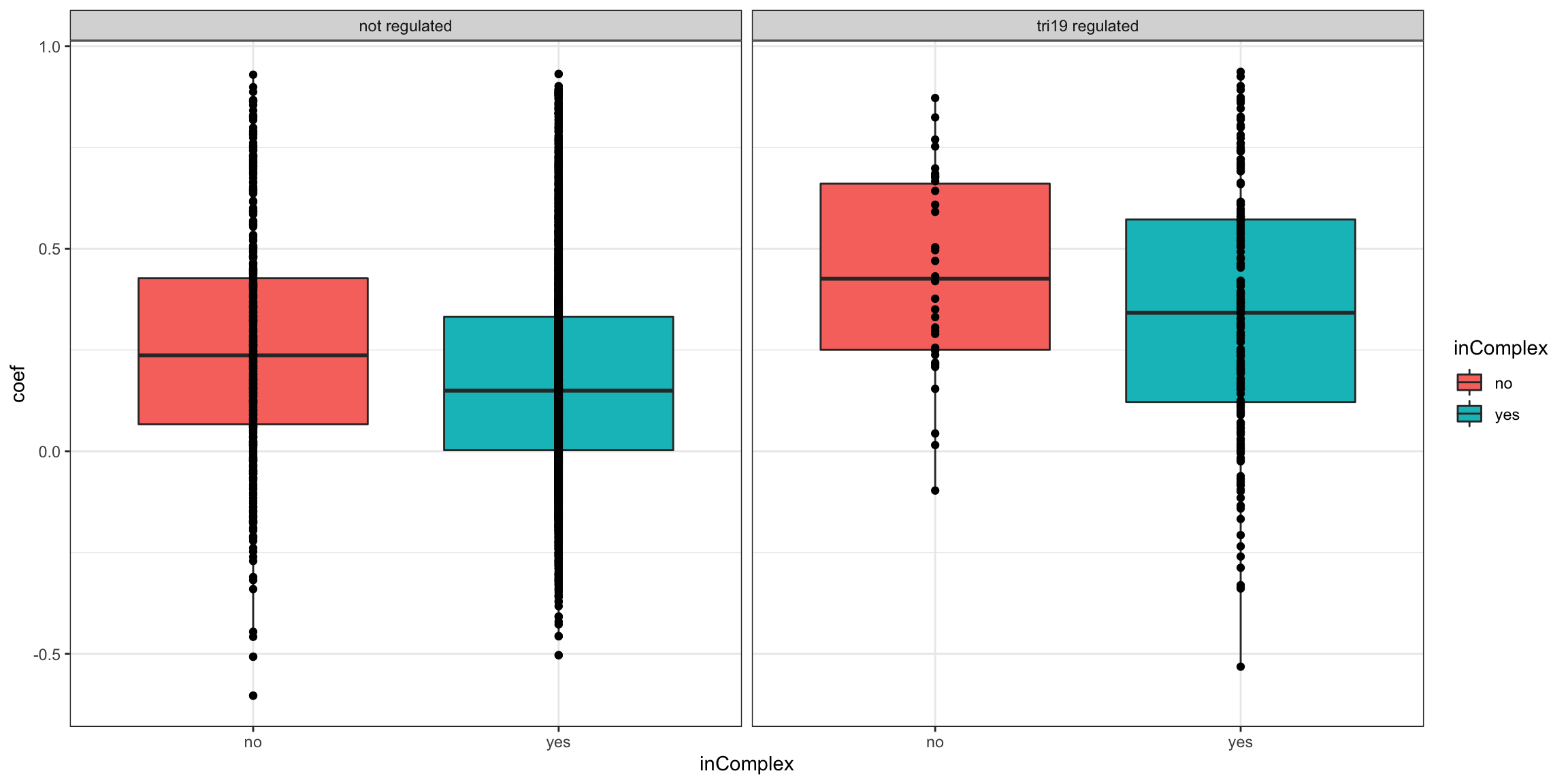
Stratified by complex formation regulation
ggplot(plotTab, aes(x=tri19Regulated, y = coef))+geom_boxplot(aes(fill = tri19Regulated)) + geom_point() +
theme_bw() + facet_wrap(~inComplex)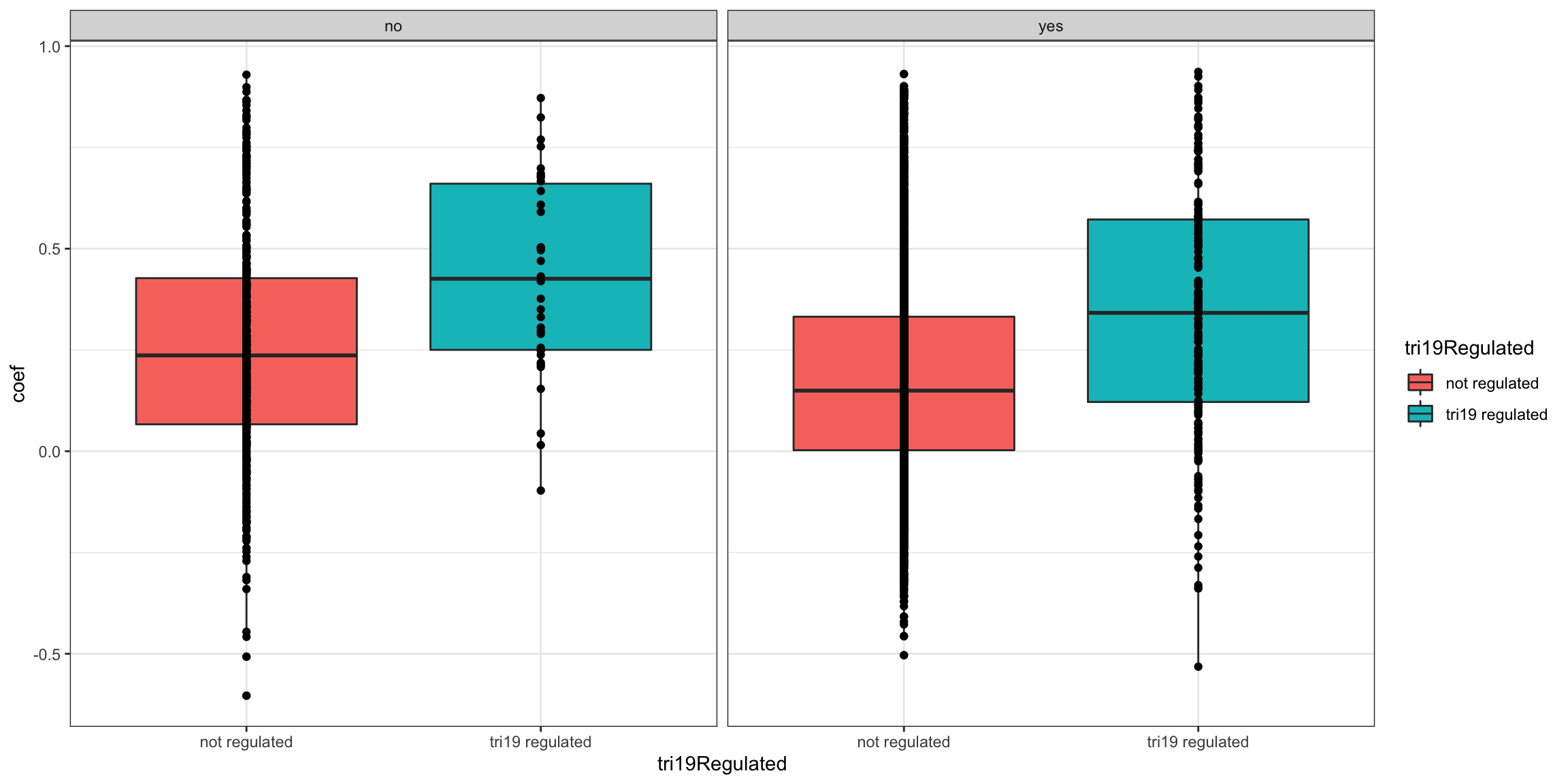
summary(lm(coef~ 1+ tri19Regulated+inComplex, plotTab))
Call:
lm(formula = coef ~ 1 + tri19Regulated + inComplex, data = plotTab)

Residuals:
     Min       1Q   Median       3Q      Max
-0.87432 -0.17904 -0.02807  0.15836  0.75209

Coefficients:
                              Estimate Std. Error t value Pr(>|t|)
(Intercept)                    0.25706    0.01142  22.518  < 2e-16 ***
tri19Regulatedtri19 regulated  0.16333    0.01712   9.542  < 2e-16 ***
inComplexyes                  -0.07795    0.01208  -6.453 1.22e-10 ***
---
Signif. codes:  0 '***' 0.001 '**' 0.01 '*' 0.05 '.' 0.1 ' ' 1

Residual standard error: 0.2518 on 4230 degrees of freedom
Multiple R-squared:  0.03109,   Adjusted R-squared:  0.03063
F-statistic: 67.87 on 2 and 4230 DF,  p-value: < 2.2e-16
Same as trisomy12
Test association under different conditions
testCor <- function(rnaMat, proMat, gene) {
  geneOverlap <- intersect(rownames(rnaMat),rownames(proMat))

  #subset genes
  rnaMat <- rnaMat[geneOverlap,]
  proMat <- proMat[geneOverlap,]

  #get group
  geneVec <- patMeta[match(colnames(proMat),patMeta$Patient.ID),][[gene]]

  resTab <- lapply(levels(geneVec), function(l) {
    rnaSub <- rnaMat[,geneVec %in% l]
    proSub <- proMat[,geneVec %in% l]
    eachRes <- lapply(geneOverlap, function(i) {
      rna <- rnaSub[i,]
      pro <- proSub[i,]
      res <- cor(rna, pro, use = "pairwise.complete.obs")
      data.frame(id = i, coef = res, stringsAsFactors = FALSE)
    }) %>% bind_rows() %>% mutate(variant = gene, group = l)
  }) %>% bind_rows() %>%
    mutate(symbol = rowData(dds[id,])$symbol,
           chr = rowData(dds[id,])$chromosome,
           group=factor(group))

  g <- ggplot(resTab, aes(x=coef, fill = group)) +
    geom_histogram(position = "identity", col = "grey50", alpha =0.3, bins =100) +
    geom_vline(xintercept = 0, col = "red", linetype = "dashed") +
    xlab("Pearson's correlation coefficient") +
    scale_fill_discrete(name = gene)

  return(list(resTab=resTab, plot=g))
}
Trisomy12
corRes <- testCor(rnaMat, proMat, "trisomy12")
corRes$plot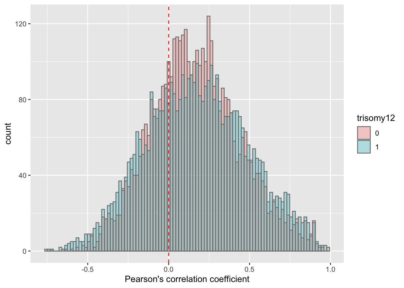 No visible difference.
Per chromosome
plotTab <- corRes$resTab
ggplot(plotTab, aes(x=coef, fill = group)) +
    geom_histogram(position = "identity", col = "grey50", alpha =0.3, bins =100) +
    geom_vline(xintercept = 0, col = "red", linetype = "dashed") +
    xlab("Pearson's correlation coefficient") +
    scale_fill_discrete(name = "trisomy12") +
  facet_wrap(~chr,ncol = 3)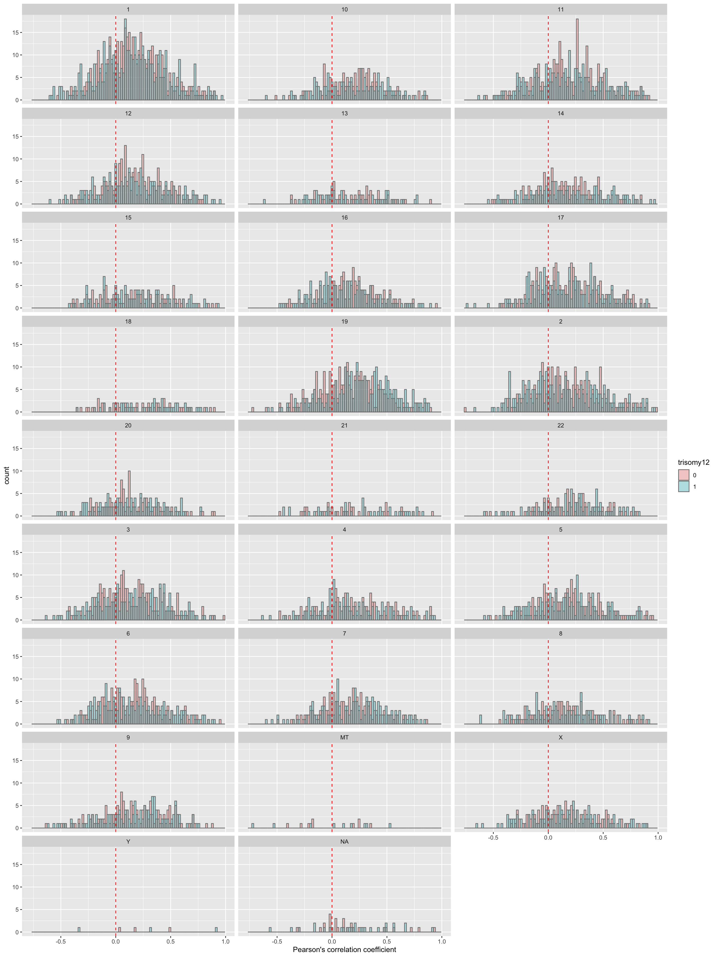
IGHV
corRes <- testCor(rnaMat, proMat, "IGHV.status")
corRes$plot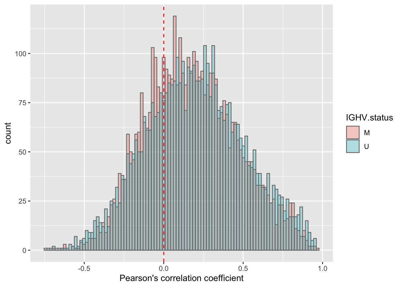 No visible difference.
Per chromosome
plotTab <- corRes$resTab
ggplot(plotTab, aes(x=coef, fill = group)) +
    geom_histogram(position = "identity", col = "grey50", alpha =0.3, bins =100) +
    geom_vline(xintercept = 0, col = "red", linetype = "dashed") +
    xlab("Pearson's correlation coefficient") +
    scale_fill_discrete(name =  "IGHV.status") +
  facet_wrap(~chr,ncol = 3)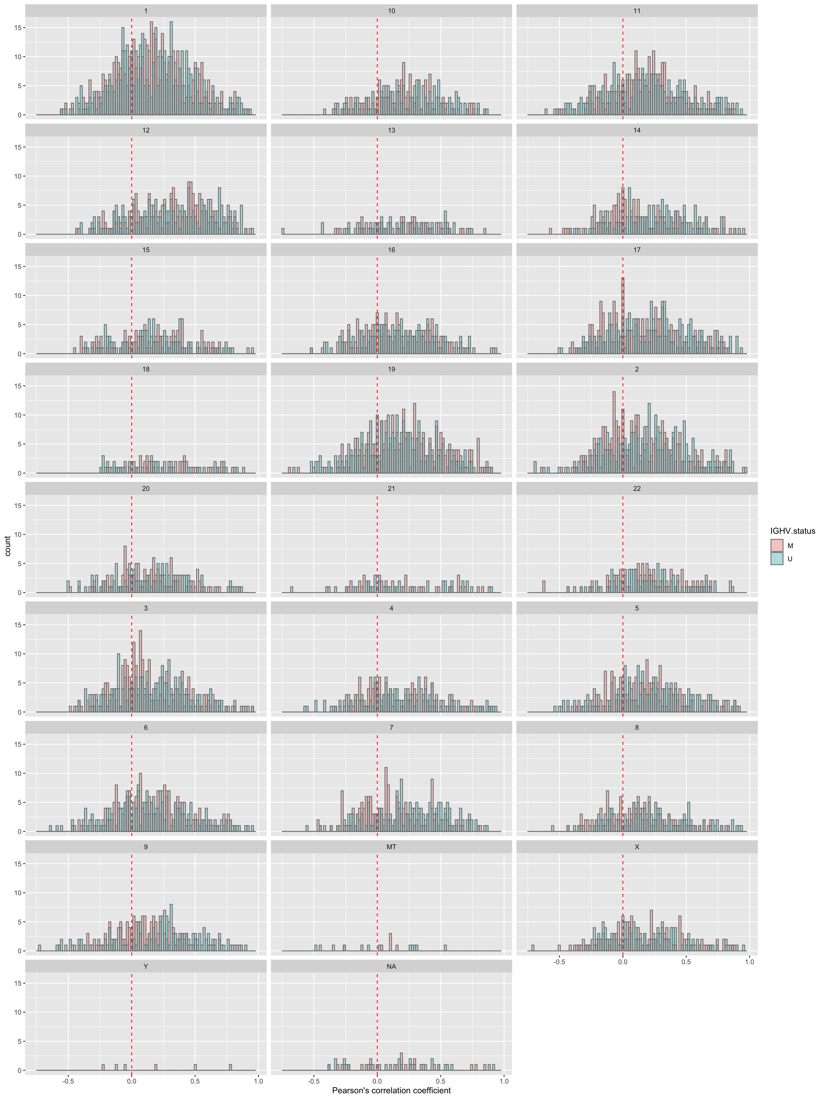
TP53
corRes <- testCor(rnaMat, proMat, "TP53")
corRes$plot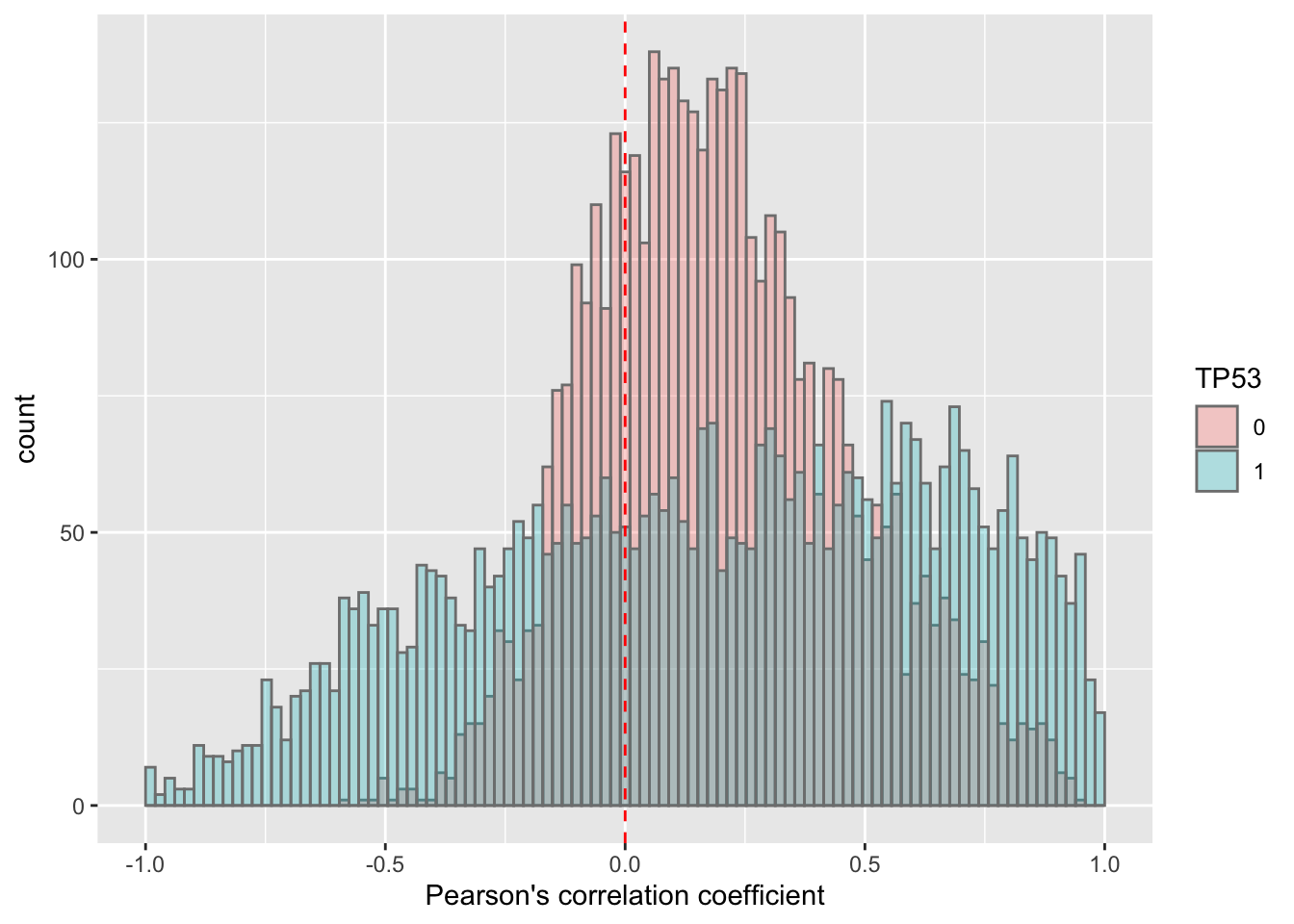 It seems there’s a difference, but note that the correlation coefficient is highly dependent on number of observations. As there’s a large difference in sample sizes between TP53 mut and WT samples, the difference in the distribution of coefficient can be confounded by sample size, and therefore not reliable.
Per chromosome
plotTab <- corRes$resTab
ggplot(plotTab, aes(x=coef, fill = group)) +
    geom_histogram(position = "identity", col = "grey50", alpha =0.3, bins =100) +
    geom_vline(xintercept = 0, col = "red", linetype = "dashed") +
    xlab("Pearson's correlation coefficient") +
    scale_fill_discrete(name = "TP53") +
  facet_wrap(~chr,ncol = 3)
SF3B1
corRes <- testCor(rnaMat, proMat, "SF3B1")
corRes$plot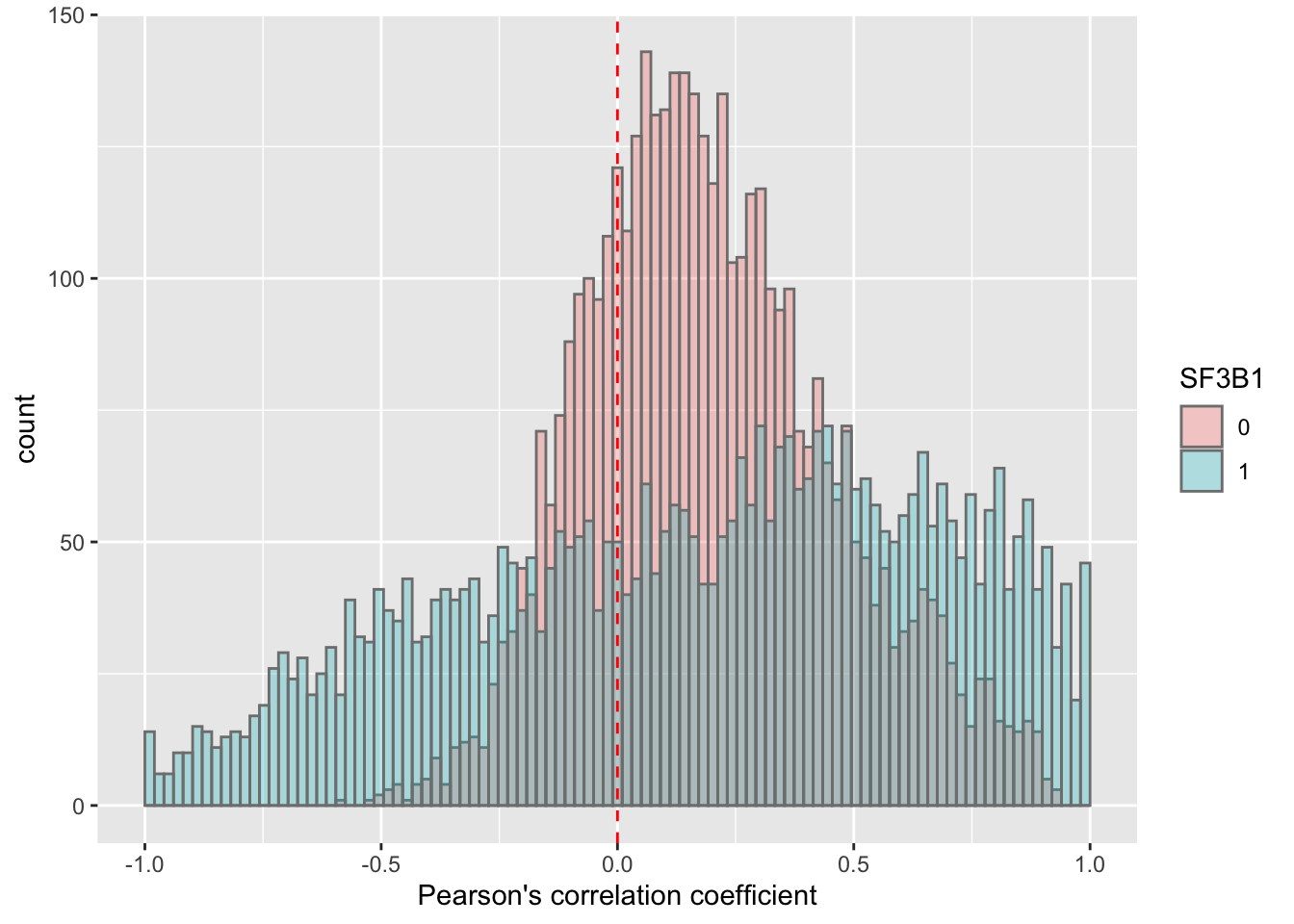 Similar to TP53. I don’t think the difference observed here is reliable.
Per chromosome
plotTab <- corRes$resTab
ggplot(plotTab, aes(x=coef, fill = group)) +
    geom_histogram(position = "identity", col = "grey50", alpha =0.3, bins =100) +
    geom_vline(xintercept = 0, col = "red", linetype = "dashed") +
    xlab("Pearson's correlation coefficient") +
    scale_fill_discrete(name = "SF3B1") +
  facet_wrap(~chr,ncol = 3)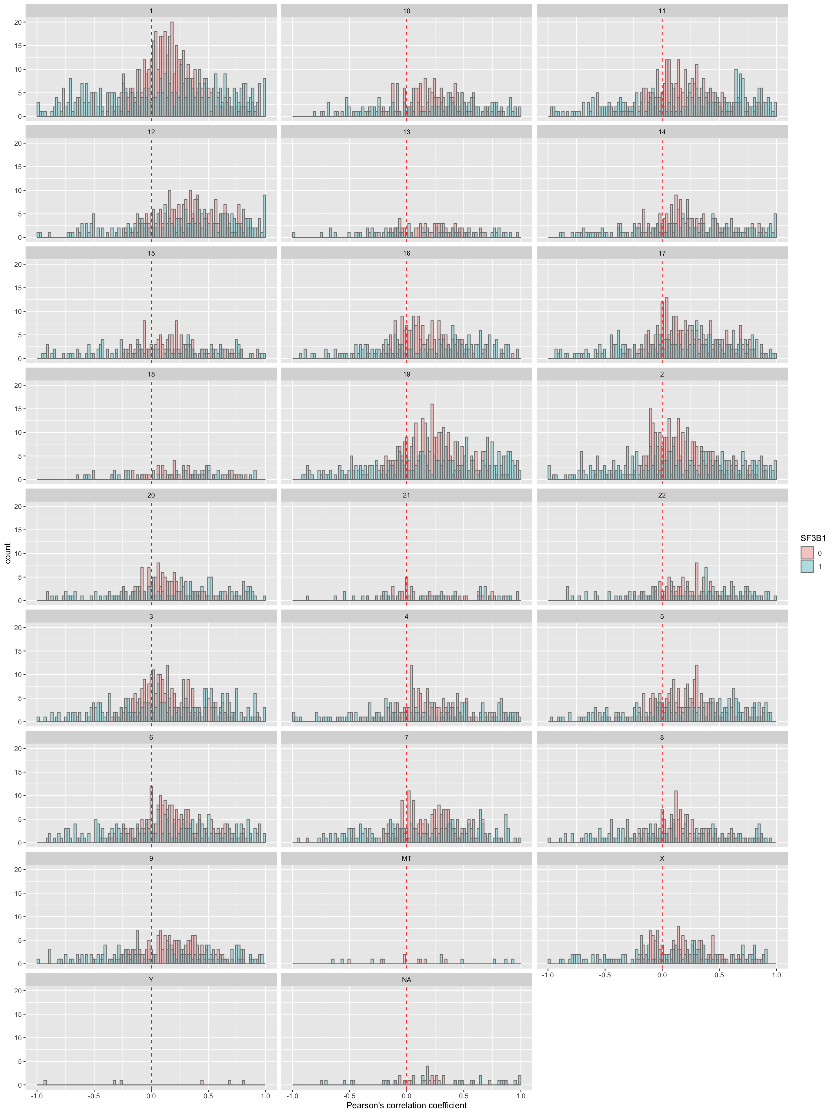
sessionInfo()R version 3.6.0 (2019-04-26)
Platform: x86_64-apple-darwin15.6.0 (64-bit)
Running under: macOS 10.15.4
Matrix products: default
BLAS: /Library/Frameworks/R.framework/Versions/3.6/Resources/lib/libRblas.0.dylib
LAPACK: /Library/Frameworks/R.framework/Versions/3.6/Resources/lib/libRlapack.dylib
locale:
[1] en_US.UTF-8/en_US.UTF-8/en_US.UTF-8/C/en_US.UTF-8/en_US.UTF-8
attached base packages:
[1] parallel stats4 stats graphics grDevices utils datasets
[8] methods base
other attached packages:
[1] forcats_0.4.0 stringr_1.4.0
[3] dplyr_0.8.5 purrr_0.3.3
[5] readr_1.3.1 tidyr_1.0.0
[7] tibble_3.0.0 ggplot2_3.3.0
[9] tidyverse_1.3.0 proDA_1.1.2
[11] DESeq2_1.24.0 SummarizedExperiment_1.14.0
[13] DelayedArray_0.10.0 BiocParallel_1.18.0
[15] matrixStats_0.54.0 Biobase_2.44.0
[17] GenomicRanges_1.36.0 GenomeInfoDb_1.20.0
[19] IRanges_2.18.1 S4Vectors_0.22.0
[21] BiocGenerics_0.30.0 jyluMisc_0.1.5
[23] limma_3.40.2
loaded via a namespace (and not attached):
[1] readxl_1.3.1 backports_1.1.4 Hmisc_4.2-0
[4] fastmatch_1.1-0 drc_3.0-1 workflowr_1.6.0
[7] igraph_1.2.4.1 shinydashboard_0.7.1 splines_3.6.0
[10] TH.data_1.0-10 digest_0.6.19 htmltools_0.4.0
[13] gdata_2.18.0 memoise_1.1.0 magrittr_1.5
[16] checkmate_2.0.0 cluster_2.1.0 openxlsx_4.1.0.1
[19] annotate_1.62.0 modelr_0.1.5 sandwich_2.5-1
[22] piano_2.0.2 colorspace_1.4-1 rvest_0.3.5
[25] blob_1.1.1 haven_2.2.0 xfun_0.8
[28] crayon_1.3.4 RCurl_1.95-4.12 jsonlite_1.6
[31] genefilter_1.66.0 survival_2.44-1.1 zoo_1.8-6
[34] glue_1.3.2 survminer_0.4.4 gtable_0.3.0
[37] zlibbioc_1.30.0 XVector_0.24.0 car_3.0-3
[40] abind_1.4-5 scales_1.1.0 mvtnorm_1.0-11
[43] DBI_1.0.0 relations_0.6-8 Rcpp_1.0.1
[46] plotrix_3.7-6 xtable_1.8-4 cmprsk_2.2-8
[49] htmlTable_1.13.1 bit_1.1-14 foreign_0.8-71
[52] km.ci_0.5-2 Formula_1.2-3 DT_0.7
[55] httr_1.4.1 htmlwidgets_1.3 fgsea_1.10.0
[58] gplots_3.0.1.1 RColorBrewer_1.1-2 acepack_1.4.1
[61] ellipsis_0.2.0 farver_2.0.3 XML_3.98-1.20
[64] pkgconfig_2.0.2 dbplyr_1.4.2 nnet_7.3-12
[67] locfit_1.5-9.1 labeling_0.3 AnnotationDbi_1.46.0
[70] tidyselect_1.0.0 rlang_0.4.5 later_0.8.0
[73] munsell_0.5.0 cellranger_1.1.0 tools_3.6.0
[76] visNetwork_2.0.7 cli_1.1.0 RSQLite_2.1.1
[79] generics_0.0.2 broom_0.5.2 evaluate_0.14
[82] yaml_2.2.0 bit64_0.9-7 knitr_1.23
[85] fs_1.4.0 zip_2.0.2 survMisc_0.5.5
[88] caTools_1.17.1.2 nlme_3.1-140 mime_0.7
[91] slam_0.1-45 xml2_1.2.2 compiler_3.6.0
[94] rstudioapi_0.10 curl_3.3 ggsignif_0.5.0
[97] marray_1.62.0 reprex_0.3.0 geneplotter_1.62.0
[100] stringi_1.4.3 lattice_0.20-38 Matrix_1.2-17
[103] shinyjs_1.0 KMsurv_0.1-5 vctrs_0.2.4
[106] pillar_1.4.3 lifecycle_0.2.0 data.table_1.12.2
[109] cowplot_0.9.4 bitops_1.0-6 httpuv_1.5.1
[112] extraDistr_1.8.11 R6_2.4.0 latticeExtra_0.6-28
[115] promises_1.0.1 KernSmooth_2.23-15 gridExtra_2.3
[118] rio_0.5.16 codetools_0.2-16 MASS_7.3-51.4
[121] gtools_3.8.1 exactRankTests_0.8-30 assertthat_0.2.1
[124] rprojroot_1.3-2 withr_2.1.2 multcomp_1.4-10
[127] GenomeInfoDbData_1.2.1 mgcv_1.8-28 hms_0.5.2
[130] grid_3.6.0 rpart_4.1-15 rmarkdown_1.13
[133] carData_3.0-2 git2r_0.26.1 maxstat_0.7-25
[136] ggpubr_0.2.1 sets_1.0-18 lubridate_1.7.4
[139] shiny_1.3.2 base64enc_0.1-3