Last updated: 2020-10-03

Checks: 5 2

Knit directory: Proteomics/analysis/

This reproducible R Markdown analysis was created with workflowr (version 1.6.2). The Checks tab describes the reproducibility checks that were applied when the results were created. The Past versions tab lists the development history.


The R Markdown is untracked by Git. To know which version of the R Markdown file created these results, you'll want to first commit it to the Git repo. If you're still working on the analysis, you can ignore this warning. When you're finished, you can run wflow_publish to commit the R Markdown file and build the HTML.

Great job! The global environment was empty. Objects defined in the global environment can affect the analysis in your R Markdown file in unknown ways. For reproduciblity it's best to always run the code in an empty environment.

The command set.seed(20200227) was run prior to running the code in the R Markdown file. Setting a seed ensures that any results that rely on randomness, e.g. subsampling or permutations, are reproducible.

Great job! Recording the operating system, R version, and package versions is critical for reproducibility.

The following chunks had caches available:
  • unnamed-chunk-11
  • unnamed-chunk-6
  • unnamed-chunk-7

To ensure reproducibility of the results, delete the cache directory manuscript_S3_trisomy12_cache and re-run the analysis. To have workflowr automatically delete the cache directory prior to building the file, set delete_cache = TRUE when running wflow_build() or wflow_publish().

Great job! Using relative paths to the files within your workflowr project makes it easier to run your code on other machines.

Great! You are using Git for version control. Tracking code development and connecting the code version to the results is critical for reproducibility.

The results in this page were generated with repository version 3fb50c5. See the Past versions tab to see a history of the changes made to the R Markdown and HTML files.

Note that you need to be careful to ensure that all relevant files for the analysis have been committed to Git prior to generating the results (you can use wflow_publish or wflow_git_commit). workflowr only checks the R Markdown file, but you know if there are other scripts or data files that it depends on. Below is the status of the Git repository when the results were generated:


Ignored files:
    Ignored:    .DS_Store
    Ignored:    .Rhistory
    Ignored:    .Rproj.user/
    Ignored:    analysis/.DS_Store
    Ignored:    analysis/.Rhistory
    Ignored:    analysis/correlateCLLPD_cache/
    Ignored:    analysis/lassoForSTAT2_cache/
    Ignored:    analysis/manuscript_S1_Overview_cache/
    Ignored:    analysis/manuscript_S2_genomicAssociation_oldTimsTOF_cache/
    Ignored:    analysis/manuscript_S3_trisomy12_cache/
    Ignored:    analysis/manuscript_S4_IGHV_cache/
    Ignored:    analysis/manuscript_S4_IGHV_oldTimsTOF_cache/
    Ignored:    analysis/manuscript_S5_trisomy19_cache/
    Ignored:    analysis/manuscript_S6_del11q_cache/
    Ignored:    analysis/manuscript_S6_del11q_oldTimsTOF_cache/
    Ignored:    analysis/manuscript_S7_SF3B1_cache/
    Ignored:    analysis/manuscript_S8_drugResponse_Outcomes_cache/
    Ignored:    analysis/manuscript_S9_STAT2_cache/
    Ignored:    code/.Rhistory
    Ignored:    data/.DS_Store
    Ignored:    output/.DS_Store

Untracked files:
    Untracked:  analysis/.trisomy12_norm.pdf
    Untracked:  analysis/CNVanalysis_11q.Rmd
    Untracked:  analysis/CNVanalysis_trisomy12.Rmd
    Untracked:  analysis/CNVanalysis_trisomy19.Rmd
    Untracked:  analysis/STAT2_cytokines.Rmd
    Untracked:  analysis/SUGP1_splicing.svg.xml
    Untracked:  analysis/analysisDrugResponses.Rmd
    Untracked:  analysis/analysisDrugResponses_IC50.Rmd
    Untracked:  analysis/analysisPCA.Rmd
    Untracked:  analysis/analysisPreliminary_LUMOS.Rmd
    Untracked:  analysis/analysisPreliminary_timsTOF_Hela.Rmd
    Untracked:  analysis/analysisPreliminary_timsTOF_new.Rmd
    Untracked:  analysis/analysisSplicing.Rmd
    Untracked:  analysis/analysisTrisomy19.Rmd
    Untracked:  analysis/annotateCNV.Rmd
    Untracked:  analysis/comparePlatforms_LUMOS_helaTimsTOF.Rmd
    Untracked:  analysis/comparePlatforms_LUMOS_newTimsTOF.Rmd
    Untracked:  analysis/comparePlatforms_newTimsTOF_helaTimsTOF.Rmd
    Untracked:  analysis/complexAnalysis_IGHV.Rmd
    Untracked:  analysis/complexAnalysis_IGHV_alternative.Rmd
    Untracked:  analysis/complexAnalysis_overall.Rmd
    Untracked:  analysis/complexAnalysis_trisomy12.Rmd
    Untracked:  analysis/complexAnalysis_trisomy12_alternative.Rmd
    Untracked:  analysis/correlateGenomic_PC12adjusted.Rmd
    Untracked:  analysis/correlateGenomic_noBlock.Rmd
    Untracked:  analysis/correlateGenomic_noBlock_MCLL.Rmd
    Untracked:  analysis/correlateGenomic_noBlock_UCLL.Rmd
    Untracked:  analysis/correlateGenomic_timsTOFnew.Rmd
    Untracked:  analysis/correlateGenomic_timsTOFnewHela.Rmd
    Untracked:  analysis/correlateRNAexpression.Rmd
    Untracked:  analysis/default.css
    Untracked:  analysis/del11q.pdf
    Untracked:  analysis/del11q_norm.pdf
    Untracked:  analysis/full_diff_list.csv
    Untracked:  analysis/lassoForSTAT2.Rmd
    Untracked:  analysis/manuscript_S0_PrepareData.Rmd
    Untracked:  analysis/manuscript_S1_Overview.Rmd
    Untracked:  analysis/manuscript_S2_genomicAssociation.Rmd
    Untracked:  analysis/manuscript_S2_genomicAssociation_oldTimsTOF.Rmd
    Untracked:  analysis/manuscript_S3_trisomy12.Rmd
    Untracked:  analysis/manuscript_S4_IGHV.Rmd
    Untracked:  analysis/manuscript_S4_IGHV_oldTimsTOF.Rmd
    Untracked:  analysis/manuscript_S5_trisomy19.Rmd
    Untracked:  analysis/manuscript_S6_del11q.Rmd
    Untracked:  analysis/manuscript_S6_del11q_oldTimsTOF.Rmd
    Untracked:  analysis/manuscript_S7_SF3B1.Rmd
    Untracked:  analysis/manuscript_S8_drugResponse_Outcomes.Rmd
    Untracked:  analysis/manuscript_S9_STAT2.Rmd
    Untracked:  analysis/peptideValidate.Rmd
    Untracked:  analysis/plotCNV_del11q.pdf
    Untracked:  analysis/plotExpressionCNV.Rmd
    Untracked:  analysis/processPeptides_LUMOS.Rmd
    Untracked:  analysis/processProteomics_timsTOF_Hela.Rmd
    Untracked:  analysis/processProteomics_timsTOF_new.Rmd
    Untracked:  analysis/protCLL.RData
    Untracked:  analysis/qualityControl_timsTOF_Hela.Rmd
    Untracked:  analysis/qualityControl_timsTOF_new.Rmd
    Untracked:  analysis/style.css
    Untracked:  analysis/tableS1_DE_proteins_p0.01.xlsx
    Untracked:  analysis/test.pdf
    Untracked:  analysis/test.svg
    Untracked:  analysis/tri12Enrich.pdf
    Untracked:  analysis/trisomy12.pdf
    Untracked:  analysis/trisomy12_AFcor.Rmd
    Untracked:  analysis/trisomy12_norm.pdf
    Untracked:  code/AlteredPQR.R
    Untracked:  code/utils.R
    Untracked:  data/190909_CLL_prot_abund_med_norm.tsv
    Untracked:  data/190909_CLL_prot_abund_no_norm.tsv
    Untracked:  data/200725_cll_diaPASEF_direct_reports/
    Untracked:  data/200728_cll_diaPASEF_direct_plus_hela_reports/
    Untracked:  data/20190423_Proteom_submitted_samples_bereinigt.xlsx
    Untracked:  data/20191025_Proteom_submitted_samples_final.xlsx
    Untracked:  data/Chemokines.csv
    Untracked:  data/IFN_list.csv
    Untracked:  data/IFNreceptor.csv
    Untracked:  data/Interleukin_receptor.csv
    Untracked:  data/Interleukins.csv
    Untracked:  data/LUMOS/
    Untracked:  data/LUMOS_peptides/
    Untracked:  data/LUMOS_protAnnotation.csv
    Untracked:  data/LUMOS_protAnnotation_fix.csv
    Untracked:  data/SampleAnnotation_cleaned.xlsx
    Untracked:  data/chemoReceptor.csv
    Untracked:  data/example_proteomics_data
    Untracked:  data/facTab_IC50atLeast3New.RData
    Untracked:  data/gmts/
    Untracked:  data/mapEnsemble.txt
    Untracked:  data/mapSymbol.txt
    Untracked:  data/proteins_in_complexes
    Untracked:  data/pyprophet_export_aligned.csv
    Untracked:  data/timsTOF_protAnnotation.csv
    Untracked:  output/Fig1A.pdf
    Untracked:  output/Fig1A.png
    Untracked:  output/Fig1A.pptx
    Untracked:  output/LUMOS_processed.RData
    Untracked:  output/MSH6_splicing.svg
    Untracked:  output/SUGP1_splicing.eps
    Untracked:  output/SUGP1_splicing.pdf
    Untracked:  output/SUGP1_splicing.svg
    Untracked:  output/cnv_plots.zip
    Untracked:  output/cnv_plots/
    Untracked:  output/cnv_plots_norm.zip
    Untracked:  output/ddsrna_enc.RData
    Untracked:  output/deResList.RData
    Untracked:  output/deResList_timsTOF.RData
    Untracked:  output/deResList_timsTOF_old.RData
    Untracked:  output/dxdCLL.RData
    Untracked:  output/dxdCLL2.RData
    Untracked:  output/encMap.RData
    Untracked:  output/exprCNV.RData
    Untracked:  output/exprCNV_enc.RData
    Untracked:  output/lassoResults_CPS.RData
    Untracked:  output/lassoResults_IC50.RData
    Untracked:  output/patMeta_enc.RData
    Untracked:  output/pepCLL_lumos.RData
    Untracked:  output/pepCLL_lumos_enc.RData
    Untracked:  output/pepTab_lumos.RData
    Untracked:  output/pheno1000_enc.RData
    Untracked:  output/pheno1000_main.RData
    Untracked:  output/plotCNV_allChr11_diff.pdf
    Untracked:  output/plotCNV_del11q_sum.pdf
    Untracked:  output/proteomic_LUMOS_20200227.RData
    Untracked:  output/proteomic_LUMOS_20200320.RData
    Untracked:  output/proteomic_LUMOS_20200430.RData
    Untracked:  output/proteomic_LUMOS_enc.RData
    Untracked:  output/proteomic_timsTOF_20200227.RData
    Untracked:  output/proteomic_timsTOF_Hela_20200806.RData
    Untracked:  output/proteomic_timsTOF_enc.RData
    Untracked:  output/proteomic_timsTOF_new_20200806.RData
    Untracked:  output/proteomic_timsTOF_old_enc.RData
    Untracked:  output/splicingResults.RData
    Untracked:  output/survival_enc.RData
    Untracked:  output/timsTOF_processed.RData
    Untracked:  plotCNV_del11q_diff.pdf
    Untracked:  summary/
    Untracked:  supp_latex/

Unstaged changes:
    Modified:   analysis/_site.yml
    Modified:   analysis/analysisSF3B1.Rmd
    Modified:   analysis/compareProteomicsRNAseq.Rmd
    Modified:   analysis/correlateCLLPD.Rmd
    Modified:   analysis/correlateGenomic.Rmd
    Deleted:    analysis/correlateGenomic_removePC.Rmd
    Modified:   analysis/correlateMIR.Rmd
    Modified:   analysis/correlateMethylationCluster.Rmd
    Modified:   analysis/index.Rmd
    Modified:   analysis/predictOutcome.Rmd
    Modified:   analysis/processProteomics_LUMOS.Rmd
    Modified:   analysis/qualityControl_LUMOS.Rmd

Note that any generated files, e.g. HTML, png, CSS, etc., are not included in this status report because it is ok for generated content to have uncommitted changes.


There are no past versions. Publish this analysis with wflow_publish() to start tracking its development.


Overview of differentially expressed proteins

A table of associations with 10% FDR

resList <- filter(resList, Gene == "trisomy12") %>%
  mutate(adj.P.Val = adj.P.IHW) %>% #use IHW corrected P-value
  mutate(Chr = rowData(protCLL[id,])$chromosome_name)
resList %>% filter(adj.P.Val <= 0.1) %>% 
  select(name, Chr,logFC, P.Value, adj.P.Val) %>%
  mutate_if(is.numeric, formatC, digits=2) %>%
  DT::datatable()

Heatmap of differentially expressed proteins (1% FDR)

proList <- filter(resList, !is.na(name), adj.P.Val < 0.01) %>% distinct(name, .keep_all = TRUE) %>% pull(id)
plotMat <- assays(protCLL)[["QRILC"]][proList,]
rownames(plotMat) <- rowData(protCLL[proList,])$hgnc_symbol

colAnno <- filter(patMeta, Patient.ID %in% colnames(protCLL)) %>%
  select(Patient.ID, trisomy12, IGHV.status) %>%
  data.frame() %>% column_to_rownames("Patient.ID")
colAnno$trisomy12 <- ifelse(colAnno$trisomy12 %in% 1, "yes","no")

rowAnno <- rowData(protCLL)[proList,c("chromosome_name","hgnc_symbol"),drop=FALSE] %>% 
  data.frame(stringsAsFactors = FALSE) %>%
  mutate(onChr12 = ifelse(chromosome_name == "12","yes","no")) %>%
  select(hgnc_symbol, onChr12) %>% data.frame() %>% column_to_rownames("hgnc_symbol")

plotMat <- jyluMisc::mscale(plotMat, censor = 5)

annoCol <- list(trisomy12 = c(yes = "black",no = "grey80"),
                IGHV.status = c(M = colList[4], U = colList[3]),
                onChr12 = c(yes = colList[1],no = "white"))

pheatmap::pheatmap(plotMat, annotation_col = colAnno, scale = "none",
                   annotation_row = rowAnno,
                   clustering_method = "ward.D2",
                   color = colorRampPalette(c(colList[2],"white",colList[1]))(100),
                   breaks = seq(-5,5, length.out = 101), annotation_colors = annoCol, 
                   show_rownames = FALSE, show_colnames = FALSE,
                   treeheight_row = 0)

Summary of chromosome distribution (10% FDR)

plotTab <- filter(resList, adj.P.Val <=0.1) %>% mutate(change = ifelse(logFC>0,"Up regulated","Down regulated"),
                              chromosome = ifelse(Chr %in% "12","chr12","other")) %>%
  group_by(change, chromosome) %>% summarise(n = length(id))

sigNumPlot <- ggplot(plotTab, aes(x=change, y=n, fill = chromosome)) + 
  geom_bar(stat = "identity", width = 0.8,
           position = position_dodge2(width = 6),
           col = "black") +
  geom_text(aes(label=n), 
            position = position_dodge(width = 0.9),
            size=4, hjust=-0.1)  +
  scale_fill_manual(name = "", labels = c("chr12","other"), values = colList) +
  coord_flip(ylim = c(0,600), expand = FALSE) + xlab("") + ylab("Number of significant associations (10% FDR)") + theme_half 
sigNumPlot

Volcano plot

plotTab <- resList 
nameList <- c("PTPN11", "PLCG1", "GRB2", "SMAD2", "PYCARD", "STAT2")
tri12Vocano <- plotVolcano(plotTab, fdrCut =0.1, x_lab="log2FoldChange", posCol = colList[1], negCol = colList[2],
            plotTitle = "trisomy12", ifLabel = TRUE, labelList = nameList)
tri12Vocano

Boxplot plot of selected genes

protTab <- sumToTidy(protCLL, rowID = "uniprotID", colID = "patID")
plotTab <- protTab %>% filter(hgnc_symbol %in% nameList) %>%
  mutate(trisomy12 = patMeta[match(patID, patMeta$Patient.ID),]$trisomy12) %>%
  mutate(status = ifelse(trisomy12 %in% 1,"trisomy12","WT"),
         name = hgnc_symbol) %>%
  mutate(status = factor(status, levels = c("WT","trisomy12")))
pList <- plotBox(plotTab, pValTabel = resList, y_lab = "Protein expression")
protBoxplot <- cowplot::plot_grid(plotlist= pList, ncol=2)
protBoxplot

Enrichment analysis

Barplot of enriched pathways

gmts = list(H= "../data/gmts/h.all.v6.2.symbols.gmt",
            KEGG = "../data/gmts/c2.cp.kegg.v6.2.symbols.gmt")
inputTab <- resList %>% filter(adj.P.Val < 0.1, Gene == "trisomy12") %>%
  mutate(name = rowData(protCLL[id,])$hgnc_symbol) %>% filter(!is.na(name)) %>%
  distinct(name, .keep_all = TRUE) %>%
  select(name, t) %>% data.frame() %>% column_to_rownames("name")
enRes <- list()
enRes[["Proteins associated with trisomy12"]] <- runGSEA(inputTab, gmts$H, "page")

p <- plotEnrichmentBar(enRes[[1]], pCut =0.1, ifFDR= TRUE, setName = "HALLMARK gene set", 
                       title = names(enRes)[1], removePrefix = "HALLMARK_", insideLegend=TRUE)
tri12Enrich <- cowplot::plot_grid(p)
tri12Enrich

Heatmaps of protein expression in enriched pathways

resList.sig <- filter(resList, !is.na(name), adj.P.Val < 0.1) %>% distinct(name, .keep_all = TRUE) 
plotMat <- assays(protCLL)[["QRILC"]][resList.sig$id,]
rownames(plotMat) <- rowData(protCLL[rownames(plotMat),])$hgnc_symbol
colAnno <- filter(patMeta, Patient.ID %in% colnames(protCLL)) %>%
  select(Patient.ID, trisomy12) %>%
  data.frame() %>% column_to_rownames("Patient.ID")
colAnno$trisomy12 <- ifelse(colAnno$trisomy12 %in% 1, "yes","no")

rowAnno <- rowData(protCLL)[resList.sig$id,c("chromosome_name","hgnc_symbol"),drop=FALSE] %>% 
  data.frame(stringsAsFactors = FALSE) %>%
  mutate(onChr12 = ifelse(chromosome_name == "12","yes","no")) %>%
  select(hgnc_symbol, onChr12) %>% data.frame() %>% column_to_rownames("hgnc_symbol")

plotMat <- jyluMisc::mscale(plotMat, censor = 5)

annoCol <- list(trisomy12 = c(yes = "black",no = "grey80"),
                IGHV.status = c(M = colList[3], U = colList[4]),
                onChr12 = c(yes = colList[1],no = "white"))
plotSetHeatmap(resList.sig, gmts$H, "HALLMARK_PI3K_AKT_MTOR_SIGNALING", plotMat, 
               colAnno, rowAnno = rowAnno, annoCol = annoCol, highLight = nameList)

plotSetHeatmap(resList.sig, gmts$H, "HALLMARK_MTORC1_SIGNALING", plotMat, colAnno, rowAnno = rowAnno, annoCol = annoCol,
                highLight = nameList)

Compare with RNA sequencing data

Buffering of gene dosage effect

Visualizing gene dosage effect on protein and RNA level

#Prepare data
load("../output/exprCNV_enc.RData")


protExprTab <- allProtTab %>% mutate(type = "Protein")
rnaExprTab <- filter(allRnaTab, id %in% protExprTab$id) %>% mutate(type = "RNA")

comExprTab <- bind_rows(rnaExprTab, protExprTab) %>%
  mutate(trisomy12 = patMeta[match(patID, patMeta$Patient.ID),]$trisomy12) %>%
  filter(!is.na(trisomy12)) %>% mutate(cnv = ifelse(trisomy12 %in% 1, "trisomy12","WT"))

In the plots below, the RNAseq dataset is subsetted for genes that also present in proteomic dataset. The plots will look somewhat different in all genes are used. But the trend is the same

Proteins/RNAs on Chr12 have higher expressions in trisomy12 samples compared to other samples

plotTab <- filter(comExprTab, ChromID %in% "chr12") %>%
  group_by(id,type) %>% mutate(med=mean(expr)) %>% mutate(expr = (expr-med)) %>%
  group_by(id, symbol, cnv, type) %>% summarise(meanExpr = mean(expr, na.rm=TRUE)) %>%
  ungroup()

dosagePlot <- ggplot(plotTab, aes(x=meanExpr, fill = cnv, col=cnv)) + 
  geom_histogram(position = "identity", alpha=0.5) + facet_wrap(~type, scale = "free") +
  scale_fill_manual(values = c(WT = "grey80", trisomy12 = colList[1]), name = "") +
  scale_color_manual(values = c(WT = "grey80", trisomy12 = colList[1]), name = "") +
  theme_full + xlab("Deviation to mean expression") +
  theme(strip.text = element_text(size =20))

dosagePlot

The variation of expression is higher in RNA than protein

(Maybe figures for supplement)

For proteins/RNA on chr12

plotTab <- filter(comExprTab, ChromID %in% "chr12") %>%
  group_by(id, symbol, type) %>% summarise(varExp = sd(expr, na.rm=TRUE)) %>%
  ungroup()

ggplot(plotTab, aes(x=varExp,  fill = type, col=type)) + 
  geom_histogram(position = "identity", alpha=0.5) + 
  scale_fill_manual(values = c(RNA = colList[4], Protein = colList[5]), name = "") +
  scale_color_manual(values = c(RNA = colList[4], Protein = colList[5]), name = "") +
  theme_full + xlab("Standard deviation of expression")

The same trend can be oberserved for non-chr12 proteins/RNAs, but less striking

plotTab <- filter(comExprTab, !ChromID %in% "chr12") %>%
  group_by(id, symbol, type) %>% summarise(varExp = sd(expr, na.rm=TRUE)) %>%
  ungroup()

ggplot(plotTab, aes(x=varExp, fill = type, col=type)) + 
  geom_histogram(position = "identity", alpha=0.5) + 
  scale_fill_manual(values = c(RNA = colList[4], Protein = colList[5]), name = "") +
  scale_color_manual(values = c(RNA = colList[4], Protein = colList[5]), name = "") +
  theme_full + xlab("Standard deviation of expression")

The overall scale of change is higher in RNA expression than protein expression

(Maybe for supplement)

plotTab <- filter(comExprTab, ChromID %in% "chr12") %>%
  group_by(id, symbol, type, cnv) %>% summarise(meanExp = mean(expr, na.rm=TRUE)) %>%
  ungroup() %>% spread(key = cnv, value = meanExp) %>%
  mutate(log2FC = log2(trisomy12/WT))

ggplot(plotTab, aes(x=log2FC, fill = type, col=type)) + 
  geom_histogram(position = "identity", alpha=0.5, bins = 100) + 
  scale_fill_manual(values = c(RNA = colList[3], Protein = colList[4]), name = "") +
  scale_color_manual(values = c(RNA = colList[3], Protein = colList[4]), name = "") +
  coord_cartesian(xlim=c(-0.25,0.25))+
  geom_vline(xintercept = 0, col = colList[1], linetype = "dashed") +
  theme_full + xlab("log2 Fold Change")

Analyzing buffering effect

Detect buffered and non-buffered proteins

Preprocessing protein and RNA data

#subset samples and genes
overSampe <- intersect(colnames(ddsCLL), colnames(protCLL))
overGene <- intersect(rownames(ddsCLL), rowData(protCLL)$ensembl_gene_id)
ddsSub <- ddsCLL[overGene, overSampe]
protSub <- protCLL[match(overGene, rowData(protCLL)$ensembl_gene_id),overSampe]
rowData(ddsSub)$uniprotID <- rownames(protSub)[match(rownames(ddsSub),rowData(protSub)$ensembl_gene_id)]

#vst
ddsSub.vst <- varianceStabilizingTransformation(ddsSub)

Differential expression on RNA level

ddsSub$trisomy12 <- patMeta[match(ddsSub$PatID,patMeta$Patient.ID),]$trisomy12
ddsSub$IGHV <- patMeta[match(ddsSub$PatID, patMeta$Patient.ID),]$IGHV.status
design(ddsSub) <- ~ trisomy12 + IGHV
deRes <- DESeq(ddsSub, betaPrior = TRUE)
rnaRes <- results(deRes, name = "trisomy121", tidy = TRUE) %>%
  dplyr::rename(geneID = row, log2FC.rna = log2FoldChange, 
                pvalue.rna = pvalue, padj.rna = padj, stat.rna= stat) %>%
  select(geneID, log2FC.rna, pvalue.rna, padj.rna, stat.rna)

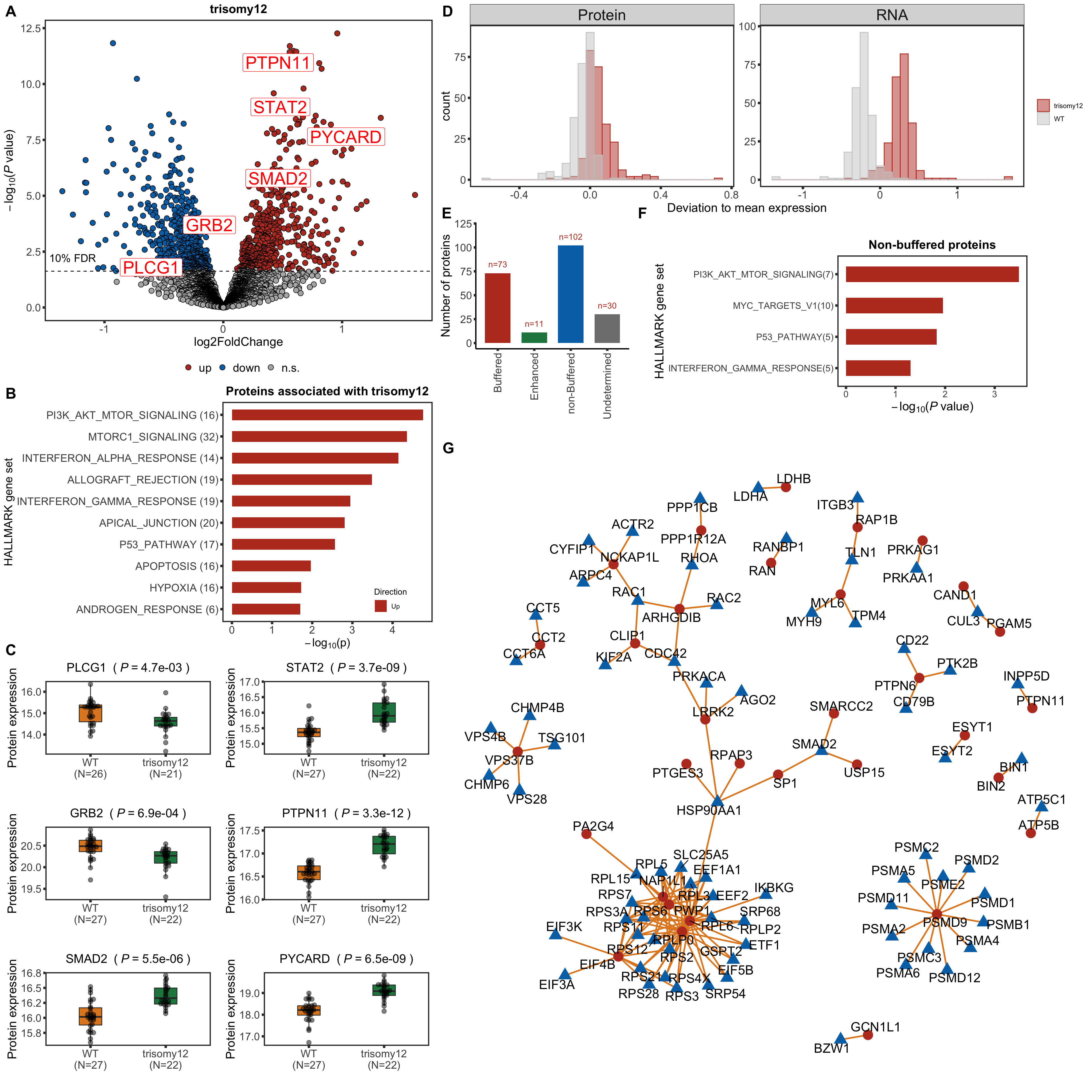
Protein abundance changes related to trisomy12

fdrCut <- 0.1
protRes <- resList %>% filter(Gene == "trisomy12") %>%
    dplyr::rename(uniprotID = id, 
                  pvalue = P.Value, padj = adj.P.IHW,
                  chrom = Chr) %>% 
    mutate(geneID = rowData(protCLL[uniprotID,])$ensembl_gene_id) %>%
    select(name, uniprotID, geneID, chrom, logFC, pvalue, padj, t) %>%
    dplyr::rename(stat =t) %>%
    arrange(pvalue) %>% as_tibble() 

Combine

allRes <- left_join(protRes, rnaRes, by = "geneID")

Only chr12 genes that are up-regulated are considered. Otherwise it's hard to intepret the dosage effect.

bufferTab <- allRes %>% filter(chrom %in% 12,stat.rna > 0) %>%
  ungroup() %>%
  mutate(stat.prot.sqrt = sqrt(stat),
         stat.prot.center = stat.prot.sqrt - mean(stat.prot.sqrt)) %>%
  mutate(score = -stat.prot.center*stat.rna) %>%
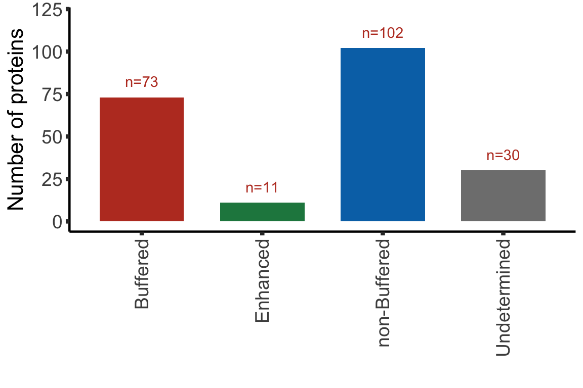
  mutate(ifBuffer = case_when(
    padj < 0.1 & padj.rna < 0.1 & stat > 0 ~ "non-Buffered",
    padj > 0.1 & padj.rna < 0.1 ~ "Buffered",
    padj < 0.1 & padj.rna > 0.1 & stat > 0 ~ "Enhanced",
    TRUE ~ "Undetermined"
  )) %>%
  arrange(desc(score))

Summary plot

sumTab <- bufferTab %>% group_by(ifBuffer) %>%
  summarise(n = length(name))

bufferPlot <- ggplot(sumTab, aes(x=ifBuffer, y = n)) + 
  geom_bar(aes(fill = ifBuffer), stat="identity", width = 0.7) + 
  geom_text(aes(label = paste0("n=", n)),vjust=-1,col=colList[1]) +
  scale_fill_manual(values =c(Buffered = colList[1],
                              Enhanced = colList[4],
                              `non-Buffered` = colList[2],
                              Undetermined = "grey50")) +
  theme_half + theme(axis.text.x = element_text(angle = 90, hjust=1, vjust=0.5),
                     legend.position = "none") +
  ylab("Number of proteins") + ylim(0,120) +xlab("")
bufferPlot

Plot example cases of buffered and non-buffered proteins

protList <- c("PTPN11","DDX51","BCAT1", "METTL7A")
geneList <- bufferTab[match(protList, bufferTab$name),]$geneID
pList <- lapply(geneList, function(i) {
  tabProt <- allProtTab %>% filter(id == i) %>%
    select(id, patID, symbol,expr) %>% dplyr::rename(protExpr = expr)
  tabRna <- allRnaTab %>% filter(id == i) %>%
    select(id, patID, expr) %>% dplyr::rename(rnaExpr = expr)
  plotTab <- left_join(tabProt, tabRna, by = c("id","patID")) %>% 
    filter(!is.na(protExpr), !is.na(rnaExpr)) %>%
    mutate(trisomy12 = patMeta[match(patID, patMeta$Patient.ID),]$trisomy12) %>%
    mutate(trisomy12 = ifelse(trisomy12 %in% 1, "yes","no"))
  p <- ggplot(plotTab, aes(x=rnaExpr, y = protExpr)) +
    geom_point(aes(col=trisomy12)) + 
    geom_smooth(formula =  y~x, method="lm",se=FALSE, color = "grey50", linetype ="dashed" ) + 
    ggtitle(unique(plotTab$symbol)) +
    ylab("Protein expression") + xlab("RNA expression") +
    scale_color_manual(values =c(yes = colList[1],no=colList[2])) +
    theme_full + theme(legend.position = "bottom")
  ggExtra::ggMarginal(p, type = "histogram", groupFill = TRUE)
  })
cowplot::plot_grid(plotlist = pList, ncol=2)

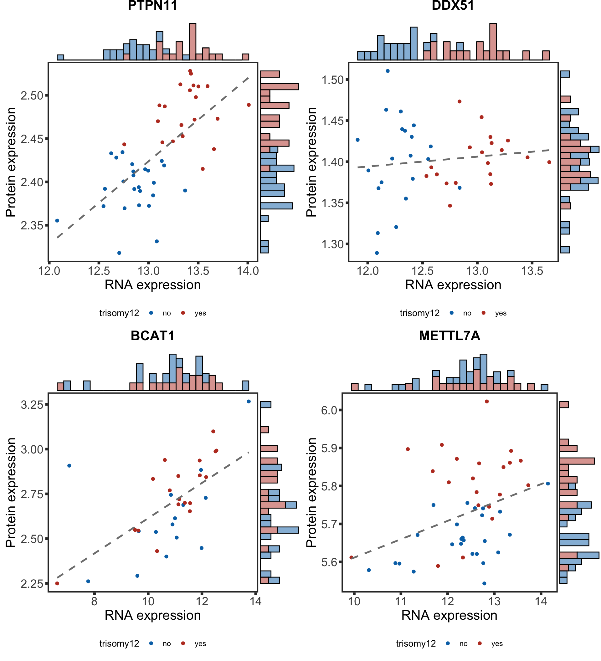
In the current analysis, I removed all the proteins that can not be unqiuely mapped. Unfortunately SLC2A14 is one of them. Can we use another example for the enhanced proteins? Like METTL7A shown here. It's a methyltransferase that has been shown to be related to innate immunity.

Enrichment of buffer and non-buffered proteins

Non-buffered prpteins

protList <- filter(bufferTab, ifBuffer == "non-Buffered")$name
refList <- unique(protExprTab$symbol)
enRes <- runFisher(protList, refList, gmts$H, pCut =0.05, ifFDR = FALSE,removePrefix = "HALLMARK_",
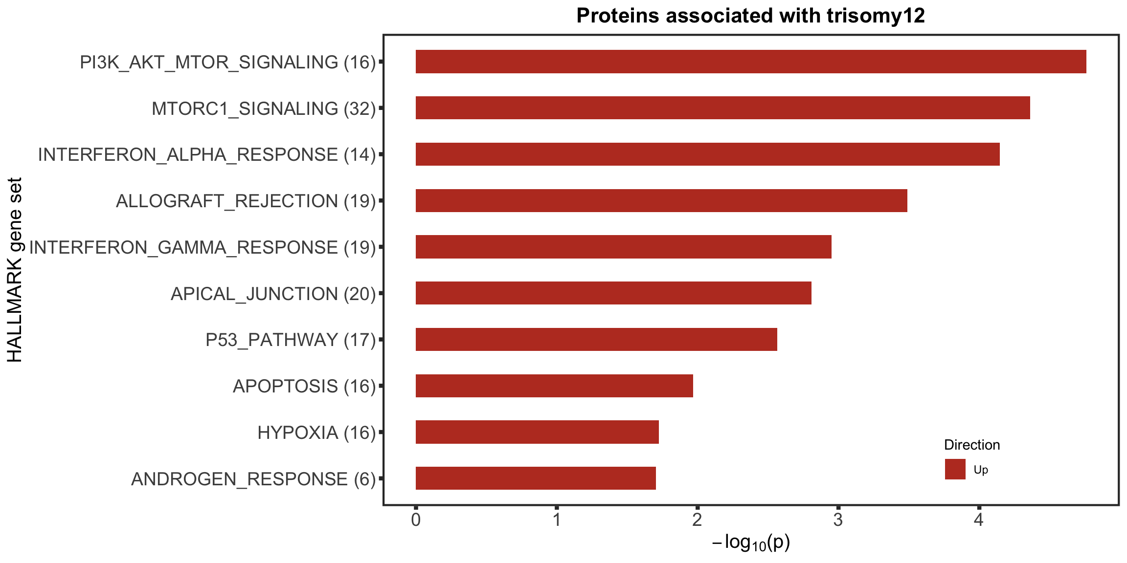
                   plotTitle = "Non-buffered proteins", insideLegend = TRUE,
                   setName = "HALLMARK gene set")
bufferEnrich <- enRes$enrichPlot + theme(plot.margin = margin(1,3,1,1, unit = "cm"))
bufferEnrich

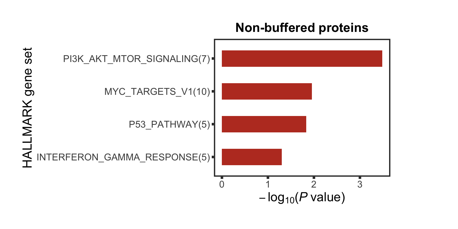
Those pathways passed p <0.05, but only PI3K_ATK_MTOR passed 10% FDR.
The result is a little different to the one ealier. Because a different enrichment method is used here, as we are not using the 'buffering score' in the manuscript.

Buffered proteins

protList <- filter(bufferTab, ifBuffer == "Buffered")$name
enRes <- runFisher(protList, refList, gmts$H, pCut =0.05, ifFDR = FALSE)
[1] "No sets passed the criteria"

No enrichment

Plot expression on genomic coordiate

load("../output/exprCNV_enc.RData")
patBack <- dplyr::filter(patMeta, Patient.ID %in% unique(allProtTab$patID)) %>%
  dplyr::select(Patient.ID, trisomy12) %>%
  dplyr::rename(patID = Patient.ID) %>%
  mutate_all(as.character) %>%
  mutate_at(vars(-patID),str_replace, "1","yes") %>%
  mutate_at(vars(-patID),str_replace, "0","no")
plotExprVar <- function(gene, chr, patBack, allBand, allLine, allProtTab, allRnaTab, protLine = NULL,
                        region = c(-Inf,Inf),ifTrend = FALSE, normalize = TRUE, maxVal =2, minVal=-2) {
  
  #table for cyto band
  bandTab <- filter(allBand, ChromID == chr, chromStart >= region[1], chromEnd <= region[2]) %>%
    mutate(chromMid = chromMid)
  
  #table for expression
  plotProtTab <- filter(allProtTab, ChromID == chr, start_position >= region[1], end_position <= region[2]) %>%
    mutate_if(is.factor,as.character)
  plotRnaTab <- filter(allRnaTab, ChromID == chr, start_position >= region[1], end_position <= region[2]) %>%
    mutate_if(is.factor,as.character)
  
  
  #summarise group mean
  plotProtTab <- plotProtTab %>% 
    mutate(group = patBack[match(patID, patBack$patID),][[gene]]) %>%
    filter(!is.na(group)) %>%
    group_by(id, group) %>% mutate(meanExpr = mean(expr, na.rm=TRUE)) %>%
    distinct(group, id,.keep_all = TRUE) %>% ungroup()

  plotRnaTab <- plotRnaTab %>%
    mutate(group = patBack[match(patID, patBack$patID),][[gene]]) %>%
    filter(!is.na(group)) %>%
    group_by(id, group) %>% mutate(meanExpr = mean(expr, na.rm=TRUE)) %>%
    distinct(group, id,.keep_all = TRUE) %>% ungroup()
  
  if (!is.null(protLine)) {
    bufferLineTab <- plotProtTab %>%
      select(symbol, mid_position, meanExpr, group) %>%
      filter(symbol %in% protLine) %>%
      pivot_wider(names_from = group, values_from = meanExpr) %>%
      mutate(lowVal = map2_dbl(yes, no, min),
             highVal = map2_dbl(yes, no, max))
  } else bufferLineTab <- NULL
  

  xMax <- max(bandTab$chromEnd, na.rm = T)
  
  #main plot for Protein
  gPro <- ggplot() + 
    geom_rect(data=bandTab, mapping=aes(xmin=chromStart, xmax=chromEnd, ymin=minVal+0.5, ymax=maxVal-0.5, 
                                        fill=Colour, label = band), alpha=0.1) +
    geom_text(data=bandTab, mapping=aes(label=band, x=chromMid), y=maxVal-0.5, hjust =1, angle = 90, size=2.5) 
    
  if (!is.null(protLine)) {
    gPro <- gPro + geom_segment(data = bufferLineTab, aes(x=mid_position, xend = mid_position, 
                                        y=lowVal, yend = highVal), linetype = "dashed") 
    
  }
  
  gPro <- gPro + geom_rect(data = plotProtTab, 
            mapping=aes(xmin=start_position,
                        xmax=end_position, ymin=meanExpr, ymax=meanExpr+0.1,
                        fill = group, label = symbol)) +
    scale_x_continuous(expand=c(0,0),limits = c(0,xMax)) +
    xlab("Genomic position [Mb]") + 
    ylab("Expression (normalized by length)") + 
    scale_fill_manual(values = c(even = "white",odd = "grey50",
                                yes = "darkred", no = "darkgreen")) +
    scale_color_manual(values = c(yes = "darkred",no = "darkgreen")) +
    ggtitle(paste0("Protein expression","(",chr,")")) +
    theme(plot.title = element_text(face = "bold", size = 10),
        legend.position = "none",
        panel.background = element_blank(),
        panel.grid.major = element_line(colour="grey90", size=0.1))
  
    if (ifTrend) {
      gPro <- gPro + geom_smooth(data =filter(plotProtTab, expr >0), 
                mapping = aes(y=meanExpr, x= mid_position,
                              color = group), 
                formula = y ~ x, method = "loess", se=FALSE, span=0.5,
                size =0.2, alpha=0.5)
    }
    
  #main plot for RNA
  gRna <- ggplot() + 
    geom_rect(data=bandTab, mapping=aes(xmin=chromStart, xmax=chromEnd, ymin=minVal, ymax=maxVal, 
                                        fill=Colour, label = band), alpha=0.1) +
    geom_text(data=bandTab, mapping=aes(label=band, x=chromMid), y=maxVal, hjust =1, angle = 90, size=2.5) +
    geom_rect(data = plotRnaTab, 
            mapping=aes(xmin=start_position,
                        xmax=end_position, ymin=meanExpr, ymax=meanExpr+0.1,
                        fill = group, label = symbol)) +
    scale_x_continuous(expand=c(0,0),limits = c(0,xMax)) +
    xlab("Genomic position [Mb]") + 
    ylab("Expression Z-score") + 
    scale_fill_manual(values = c(even = "white",odd = "grey50",
                                yes = "darkred", no = "darkgreen")) +
    scale_color_manual(values = c(yes = "darkred", no = "darkgreen")) +
    ggtitle(paste0("RNA expression","(",chr,")")) +
    theme(plot.title = element_text(face = "bold", size = 10),
        legend.position = "none",
        panel.background = element_blank(),
        panel.grid.major = element_line(colour="grey90", size=0.1))
  
    if (ifTrend) {
      gRna <- gRna + geom_smooth(data =filter(plotRnaTab), 
                mapping = aes(y=meanExpr, x= mid_position,
                              color = group), 
                formula = y ~ x, method = "loess", se=FALSE, span=0.2,
                size =0.2, alpha=0.5)
    }
    #for legend
    ## if the patient has CNV data
    lgTab <- tibble(x= seq(6),y=seq(6),
                    Expression = c(rep("yes",3), rep("no",3)))
  
    lg <- ggplot(lgTab, aes(x=x,y=y)) +
        geom_point(aes(fill = Expression), shape =22,size=3) +
        scale_fill_manual(values = c(yes = "darkred", no = "darkgreen"), name = gene) +
        theme(legend.position = "bottom")
    
    lg <- get_legend(lg)
    
    return(list(plotPro = gPro, plotRNA = gRna, legend = lg))
}

Normalize protein and RNA expression

normalized <- TRUE
#if perform normalization
if (normalized) {
  #for protein
  exprMat <- select(allProtTab,patID, id,expr) %>% 
    spread(key = patID, value =expr) %>% data.frame() %>% 
    column_to_rownames("id") %>% as.matrix()
  qm <- jyluMisc::mscale(exprMat, useMad = F)
  normTab <- data.frame(qm) %>% rownames_to_column("id") %>%
    gather(key = "patID", value = "expr", -id)
  allProtTab <- select(allProtTab, -expr) %>% left_join(normTab, by = c("patID","id"))


  #for RNA
  exprMat <- select(allRnaTab,patID, id,expr) %>% 
    spread(key = patID, value =expr) %>% data.frame() %>% 
    column_to_rownames("id") %>% as.matrix()
  qm <- jyluMisc::mscale(exprMat, useMad = F)
  normTab <- data.frame(qm) %>% rownames_to_column("id") %>%
    gather(key = "patID", value = "expr", -id)
  allRnaTab <- select(allRnaTab, -expr) %>% left_join(normTab, by = c("patID","id"))
}
#pdf("./trisomy12_norm.pdf",height = 8, width = 10)
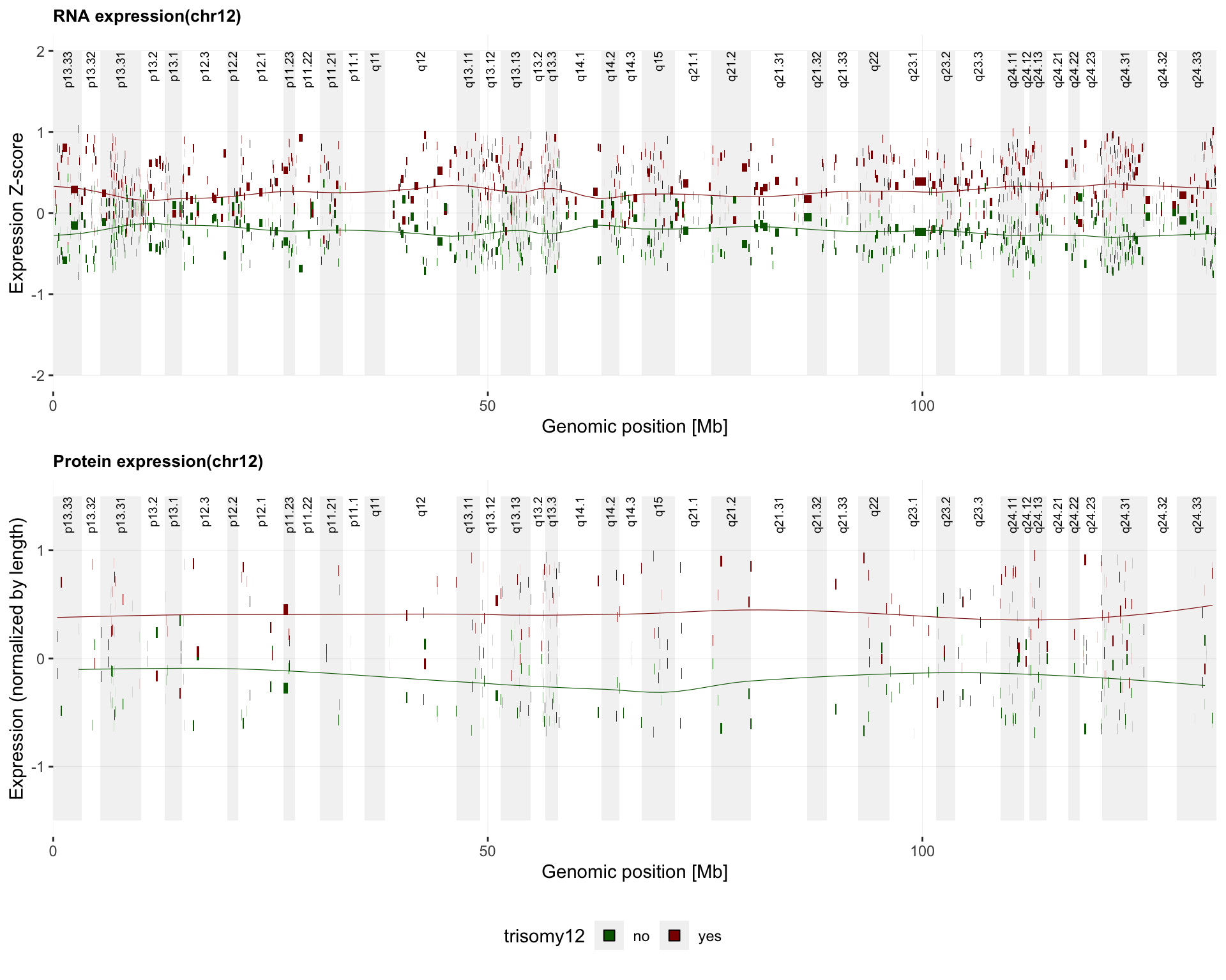
g <- plotExprVar("trisomy12","chr12",patBack,allBand, allLine, 
                 allProtTab, allRnaTab, ifTrend = TRUE)
plot_grid(g$plotRNA, g$plotPro, g$legend, ncol = 1, rel_heights = c(1,1,0.2))

#dev.off()

Protein complex analysis

Preprocessing

Processing protein complex data

int_pairs <- read_delim("../data/proteins_in_complexes", delim = "\t") %>%
  mutate(Reactome = grepl("Reactome",Evidence_supporting_the_interaction),
         Corum = grepl("Corum",Evidence_supporting_the_interaction)) %>%
  filter(ProtA %in% rownames(protSub) & ProtB %in% rownames(protSub)) %>%
  mutate(pair=map2_chr(ProtA, ProtB, ~paste0(sort(c(.x,.y)), collapse = "-"))) %>%
  mutate(database = case_when(
    Reactome & Corum ~ "both",
    Reactome & !Corum ~ "Reactome",
    !Reactome & Corum ~ "Corum",
    TRUE ~ "other"
  )) %>% mutate(inComplex = "yes")

Construct protein-protein interaction network by connecting chr12 proteins and non-chr12 protein

comTab <- int_pairs %>% select(ProtA, ProtB, database) %>%
  mutate(chrA = rowData(protCLL[ProtA,])$chromosome_name,
         chrB = rowData(protCLL[ProtB,])$chromosome_name) %>%
  filter(!is.na(chrA), !is.na(chrB)) %>%
  filter((chrA == "12" & chrB != "12") | (chrA !="12" & chrB == "12")) %>%
  mutate(source = ifelse(chrA == 12, ProtA, ProtB),
         target = ifelse(chrA == 12, ProtB, ProtA)) %>%
  select(source, target, database)
fdrCut <- 0.1
resTab <- select(allRes, name, uniprotID, chrom, padj, padj.rna, logFC,log2FC.rna) %>%
  mutate(sigProt = padj <= fdrCut,
         sigRna = padj.rna <=fdrCut,
         upProt = sigProt & logFC > 0,
         upRna = sigRna & log2FC.rna > 0)
comTab <- comTab %>% 
  left_join(resTab, by = c(source = "uniprotID")) %>%
  left_join(resTab, by = c(target = "uniprotID")) %>%
  rename_all(funs(str_replace(., "x", "source"))) %>%
  rename_all(funs(str_replace(., "y", "target"))) 
comTab.filter <- filter(comTab, sigProt.source, sigProt.target, !sigRna.target, upProt.source, upProt.target)
#get node list
allNodes <- union(comTab.filter$name.source, comTab.filter$name.target) 

nodeList <- data.frame(id = seq(length(allNodes))-1, name = allNodes, stringsAsFactors = FALSE) %>%
  mutate(onChr12 = ifelse(rowData(protCLL[match(name, rowData(protCLL)$hgnc_symbol),])$chromosome_name %in% "12", 
                          "chr12","otherChr"))

#get edge list
edgeList <- select(comTab.filter, name.source, name.target, database) %>%
  dplyr::rename(Source = name.source, Target = name.target) %>% 
  mutate(Source = nodeList[match(Source,nodeList$name),]$id,
         Target = nodeList[match(Target, nodeList$name),]$id) %>%
  data.frame(stringsAsFactors = FALSE)

net <- graph_from_data_frame(vertices = nodeList, d=edgeList, directed = FALSE)
tidyNet <- as_tbl_graph(net)
complexNet <- ggraph(tidyNet, layout = "igraph", algorithm = "nicely") + 
  geom_edge_link(color = colList[3], width=1) + 
  geom_node_point(aes(color =onChr12, shape = onChr12), size=6) + 
  geom_node_text(aes(label = name), repel = TRUE, size=6) +
  scale_color_manual(values = c(chr12 = colList[1],otherChr = colList[2])) +
  scale_edge_color_brewer(palette = "Set2") +
  theme_graph(base_family = "sans") + theme(legend.position = "none") 
complexNet

Heatmap of BCR complex proteins

seedProt <- c("CD79B","CD22","GRB2","PLCG1")
seedID <- rownames(protCLL[match(seedProt,rowData(protCLL)$hgnc_symbol),])
complexID <- filter(int_pairs, ProtA %in% seedID | ProtB %in% seedID)
resList.BCR <- filter(resList, id %in% c(complexID$ProtA, complexID$ProtB), Gene == "trisomy12",
                      adj.P.Val <= 0.1)
protList <- resList.BCR$id
plotMat <- assays(protCLL)[["QRILC"]][protList,]
rownames(plotMat) <- rowData(protCLL[protList,])$hgnc_symbol

colAnno <- filter(patMeta, Patient.ID %in% colnames(protCLL)) %>%
  select(Patient.ID, trisomy12, IGHV.status) %>%
  data.frame() %>% column_to_rownames("Patient.ID") %>%
  arrange(trisomy12)
colAnno$trisomy12 <- ifelse(colAnno$trisomy12 %in% 1, "yes","no")

plotMat <- jyluMisc::mscale(plotMat, censor = 5)
plotMat <- plotMat[,rownames(colAnno)]


rowAnno <- rowData(protCLL)[,c("chromosome_name","hgnc_symbol"),drop=FALSE] %>% 
  data.frame(stringsAsFactors = FALSE) %>%
  mutate(onChr12 = ifelse(chromosome_name == "12","yes","no")) %>%
  select(hgnc_symbol, onChr12) %>% distinct(hgnc_symbol, .keep_all = TRUE) %>%
  data.frame() %>% remove_rownames() %>%
  column_to_rownames("hgnc_symbol")

annoCol <- list(trisomy12 = c(yes = "black",no = "grey80"),
                IGHV.status = c(M = colList[4], U = colList[3]),
                onChr12 = c(yes = colList[1],no = "white"))

#pheatmap::pheatmap(plotMat, annotation_col = colAnno, scale = "none",
#                   annotation_row = rowAnno, cluster_cols = FALSE,
#                   clustering_method = "ward.D2",
#                   color = colorRampPalette(c(colList[2],"white",colList[1]))(100),
#                   breaks = seq(-5,5, length.out = 101), annotation_colors = annoCol, 
#                   show_rownames = TRUE, show_colnames = FALSE,
#                   treeheight_row = 0)

haCol <- ComplexHeatmap::HeatmapAnnotation(df = colAnno, col=annoCol, which = "column",annotation_name_gp = gpar(fontface = "bold"))
haRow <- ComplexHeatmap::HeatmapAnnotation(df = rowAnno[rownames(plotMat),,drop=FALSE], col=annoCol, which = "row", annotation_name_gp = gpar(fontface = "bold"))

labelCol <- rep("black",nrow(plotMat))
highlight <- c(seedProt, c("PTPN6","PTPN11","PTK2B"))
labelCol[rownames(plotMat) %in% highlight] <-"red"


ComplexHeatmap::Heatmap(plotMat, col = colorRampPalette(c(colList[2],"white",colList[1]))(100),name = "z-score",
                        top_annotation = haCol, left_annotation = haRow, show_column_names = FALSE,
                        cluster_columns  = FALSE, clustering_method_rows = "ward.D2",
                        row_names_gp = gpar(col = labelCol), show_row_dend = FALSE,
                        column_title_gp = gpar(cex= 1.5, fontface = "bold"))

Validation on peptide level

load("../output/pepCLL_lumos_enc.RData")
stratifier <- "trisomy12"
plotList <- lapply(nameList, function(n) {
 mutStatus <- as.character(patMeta[match(colnames(pepCLL), patMeta$Patient.ID),][[stratifier]])
 names(mutStatus) <- colnames(pepCLL)
 plotPep(pepCLL, n, type = "count", stratifier = stratifier, mutStatus = mutStatus)
})
cowplot::plot_grid(plotlist = plotList, ncol=1)

Validation using timsTOF data

Load timsTOF data

load("../output/proteomic_timsTOF_enc.RData")
load("../output/deResList_timsTOF.RData")
resList <- filter(resList, Gene == "trisomy12") %>%
  mutate(adj.P.Val = adj.P.IHW) %>% #use IHW corrected P-value
  mutate(Chr = rowData(protCLL[id,])$chromosome_name)
protTab <- sumToTidy(protCLL, rowID = "uniprotID", colID = "patID")
plotTab <- protTab %>% filter(hgnc_symbol %in% nameList) %>%
  mutate(trisomy12 = patMeta[match(patID, patMeta$Patient.ID),]$trisomy12) %>%
  mutate(status = ifelse(trisomy12 %in% 1,"trisomy12","WT"),
         name = hgnc_symbol) %>%
    mutate(status = factor(status, levels = c("WT","trisomy12")))
pList <- plotBox(plotTab, pValTabel = resList)
cowplot::plot_grid(plotlist= pList, ncol=2)

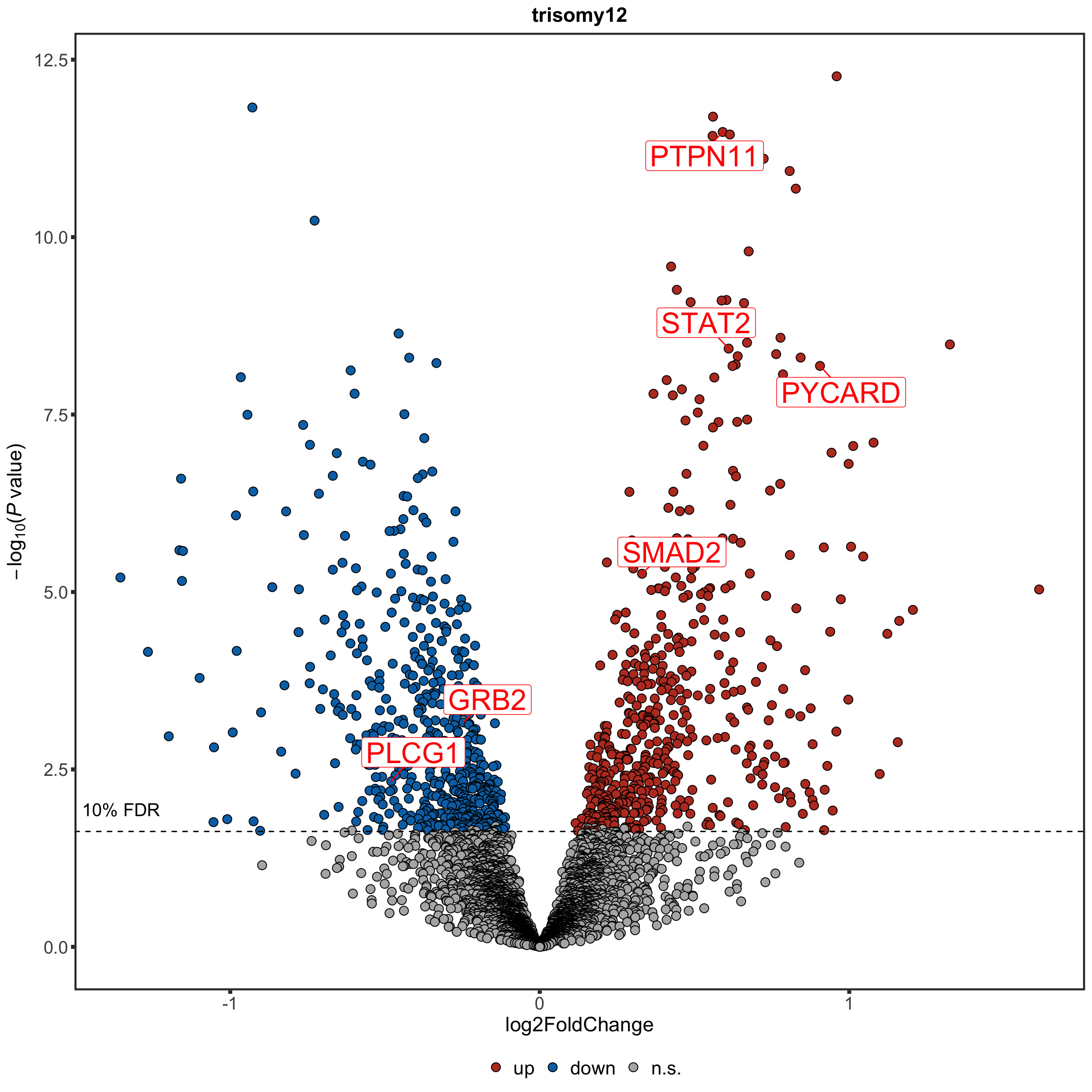
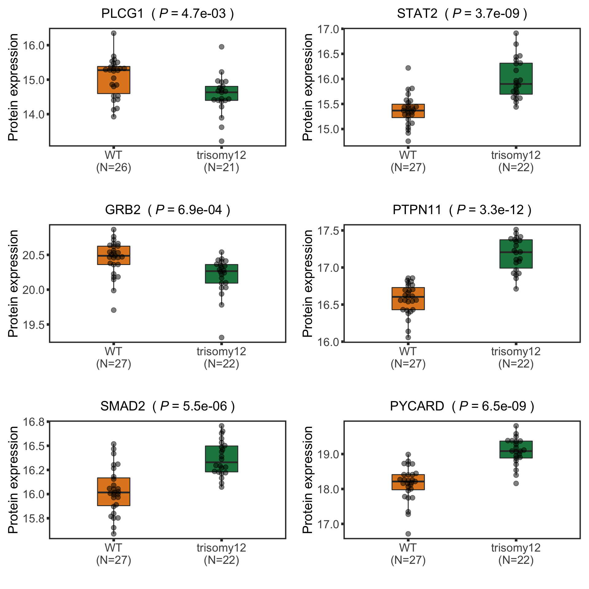
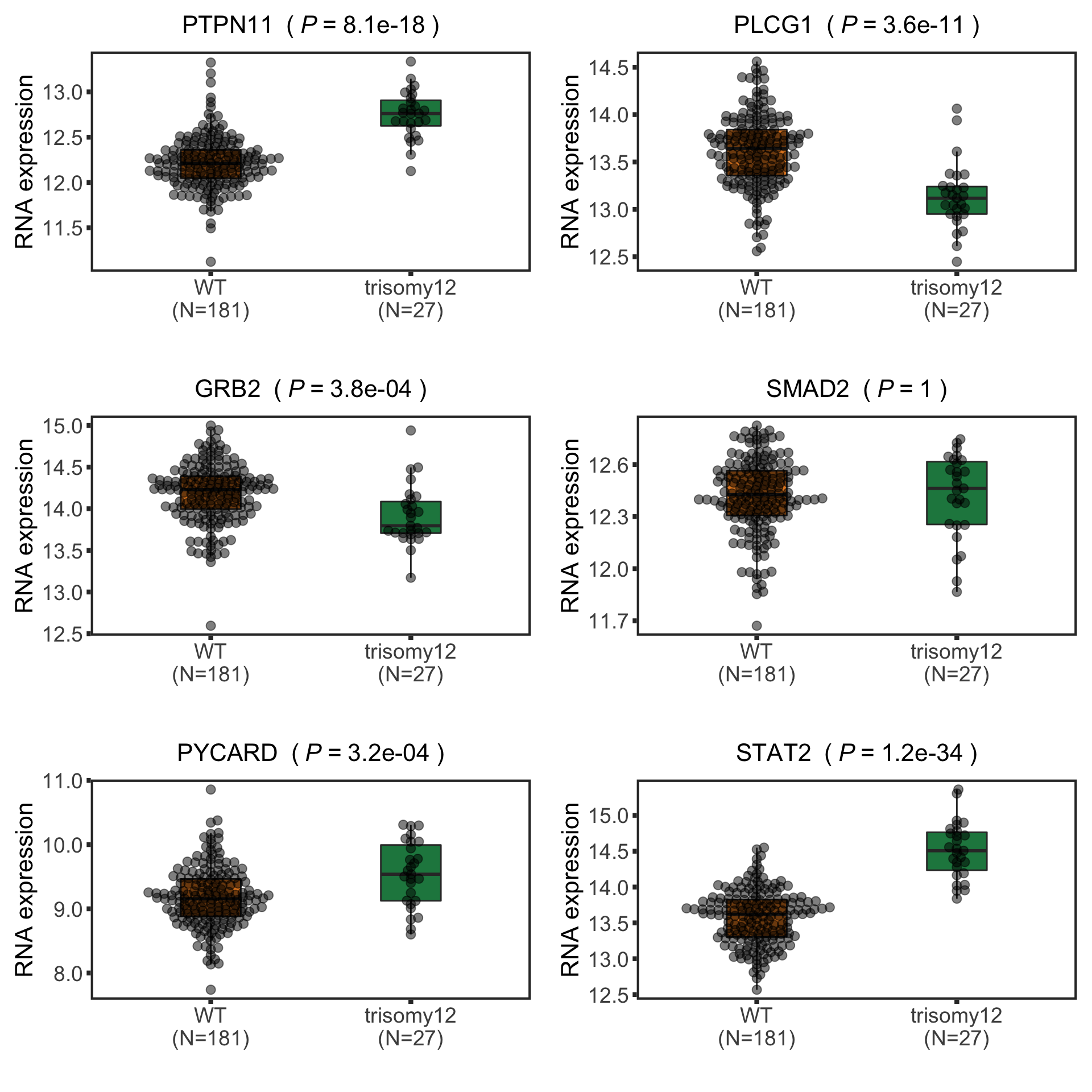
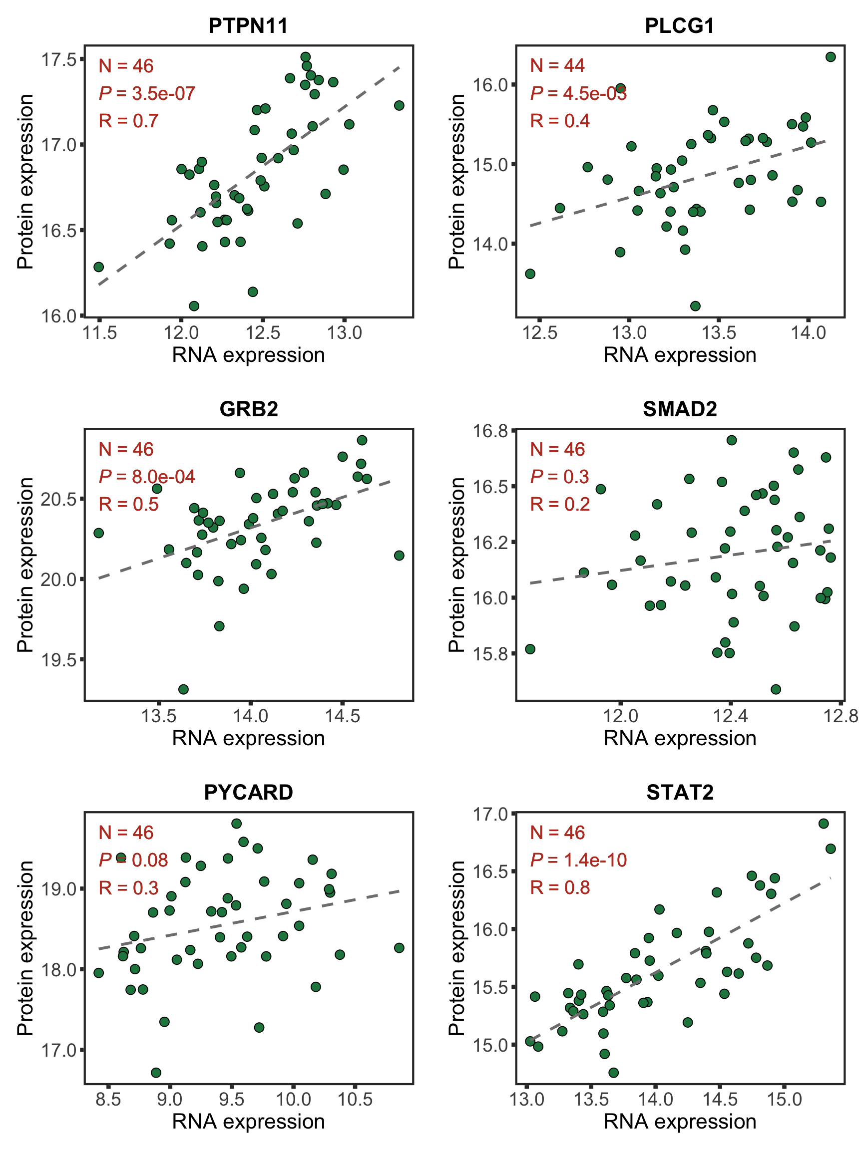
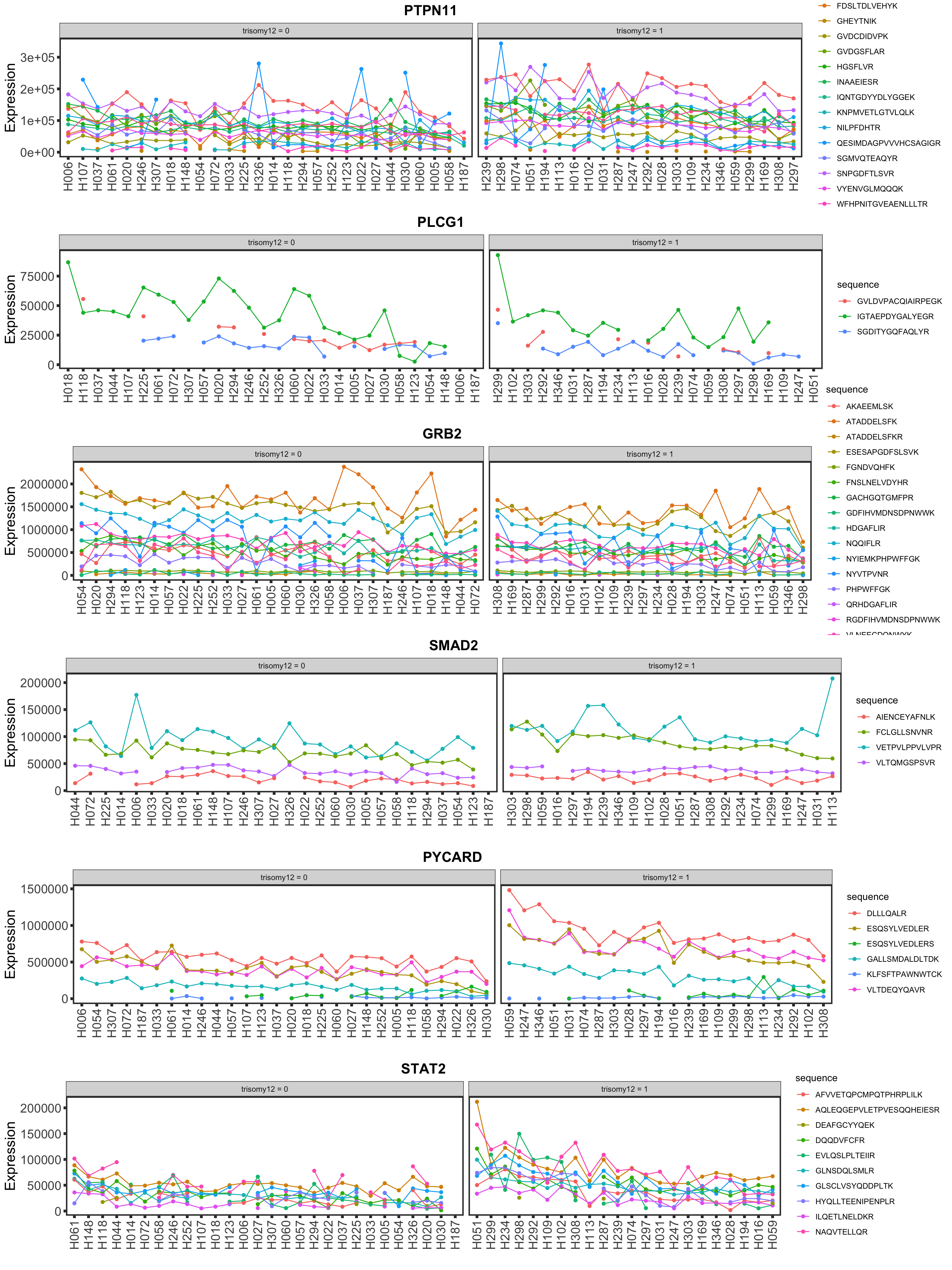
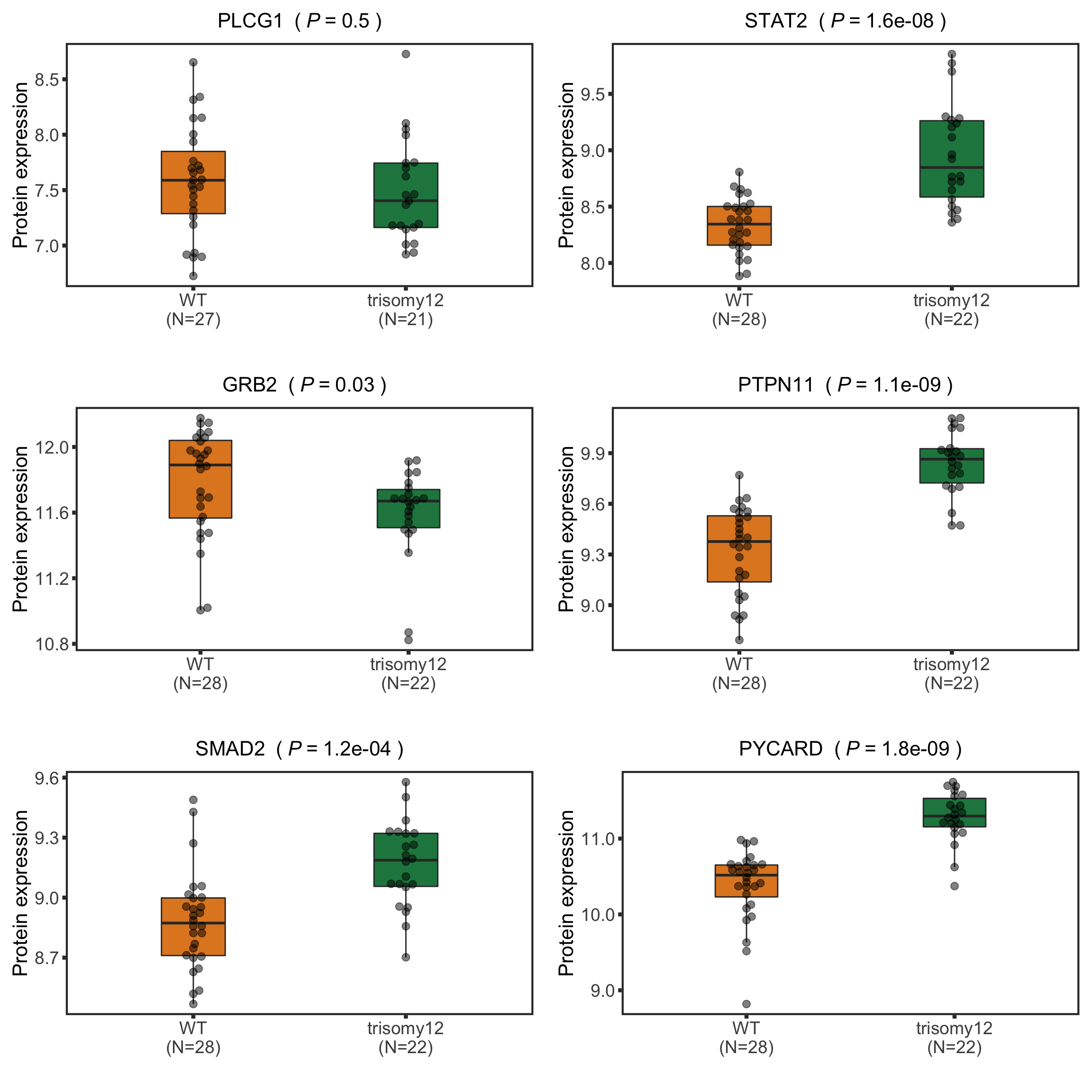
Now PLCG1 does not correlate with trisomy12, but PYCARD can be detected and correlate with trisomy12

Assemble figures

Main text figure 2

leftCol <- plot_grid(tri12Vocano, tri12Enrich,protBoxplot, ncol=1,
                     rel_heights = c(0.35,0.25,0.4),
                     labels = c("A","B","C"), label_size = 20,
                     vjust = c(1.5,1.5,0))
rightCol <- plot_grid(dosagePlot, 
                      plot_grid(bufferPlot, bufferEnrich,ncol=2, 
                                rel_widths = c(0.3,0.7), labels = c("E","F"), label_size = 20,
                                vjust = c(0,0)),
                      complexNet, ncol=1,
                      rel_heights = c(0.2,0.2,0.6), labels = c("D","","G"), label_size = 20)

#pdf("test.pdf", height = 20, width = 20)
plot_grid(leftCol, rightCol, rel_widths = c(0.4,0.6))

#dev.off()

sessionInfo()
R version 3.6.0 (2019-04-26)
Platform: x86_64-apple-darwin15.6.0 (64-bit)
Running under: macOS  10.15.6

Matrix products: default
BLAS:   /Library/Frameworks/R.framework/Versions/3.6/Resources/lib/libRblas.0.dylib
LAPACK: /Library/Frameworks/R.framework/Versions/3.6/Resources/lib/libRlapack.dylib

locale:
[1] en_US.UTF-8/en_US.UTF-8/en_US.UTF-8/C/en_US.UTF-8/en_US.UTF-8

attached base packages:
 [1] grid      parallel  stats4    stats     graphics  grDevices utils    
 [8] datasets  methods   base     

other attached packages:
 [1] piano_2.2.0                 latex2exp_0.4.0            
 [3] forcats_0.5.0               stringr_1.4.0              
 [5] dplyr_1.0.0                 purrr_0.3.4                
 [7] readr_1.3.1                 tidyr_1.1.0                
 [9] tibble_3.0.3                tidyverse_1.3.0            
[11] ggbeeswarm_0.6.0            ComplexHeatmap_2.2.0       
[13] pheatmap_1.0.12             ggraph_2.0.3               
[15] ggplot2_3.3.2               igraph_1.2.5               
[17] cowplot_1.0.0               tidygraph_1.2.0            
[19] DESeq2_1.26.0               SummarizedExperiment_1.16.1
[21] DelayedArray_0.12.3         BiocParallel_1.20.1        
[23] matrixStats_0.56.0          Biobase_2.46.0             
[25] GenomicRanges_1.38.0        GenomeInfoDb_1.22.1        
[27] IRanges_2.20.2              S4Vectors_0.24.4           
[29] BiocGenerics_0.32.0         limma_3.42.2               

loaded via a namespace (and not attached):
  [1] shinydashboard_0.7.1   tidyselect_1.1.0       RSQLite_2.2.0         
  [4] AnnotationDbi_1.48.0   htmlwidgets_1.5.1      maxstat_0.7-25        
  [7] munsell_0.5.0          codetools_0.2-16       DT_0.14               
 [10] miniUI_0.1.1.1         withr_2.2.0            colorspace_1.4-1      
 [13] knitr_1.29             rstudioapi_0.11        ggsignif_0.6.0        
 [16] labeling_0.3           git2r_0.27.1           slam_0.1-47           
 [19] GenomeInfoDbData_1.2.2 KMsurv_0.1-5           polyclip_1.10-0       
 [22] bit64_0.9-7            farver_2.0.3           rprojroot_1.3-2       
 [25] vctrs_0.3.1            generics_0.0.2         TH.data_1.0-10        
 [28] xfun_0.15              sets_1.0-18            R6_2.4.1              
 [31] clue_0.3-57            graphlayouts_0.7.0     locfit_1.5-9.4        
 [34] fgsea_1.12.0           bitops_1.0-6           assertthat_0.2.1      
 [37] promises_1.1.1         scales_1.1.1           multcomp_1.4-13       
 [40] nnet_7.3-14            ggExtra_0.9            beeswarm_0.2.3        
 [43] gtable_0.3.0           sandwich_2.5-1         workflowr_1.6.2       
 [46] rlang_0.4.7            genefilter_1.68.0      GlobalOptions_0.1.2   
 [49] splines_3.6.0          rstatix_0.6.0          acepack_1.4.1         
 [52] broom_0.7.0            checkmate_2.0.0        yaml_2.2.1            
 [55] abind_1.4-5            modelr_0.1.8           crosstalk_1.1.0.1     
 [58] backports_1.1.8        httpuv_1.5.4           Hmisc_4.4-0           
 [61] relations_0.6-9        tools_3.6.0            ellipsis_0.3.1        
 [64] gplots_3.0.4           RColorBrewer_1.1-2     Rcpp_1.0.5            
 [67] visNetwork_2.0.9       base64enc_0.1-3        zlibbioc_1.32.0       
 [70] RCurl_1.98-1.2         ggpubr_0.4.0           rpart_4.1-15          
 [73] GetoptLong_1.0.2       viridis_0.5.1          zoo_1.8-8             
 [76] haven_2.3.1            ggrepel_0.8.2          cluster_2.1.0         
 [79] exactRankTests_0.8-31  fs_1.4.2               magrittr_1.5          
 [82] data.table_1.12.8      openxlsx_4.1.5         circlize_0.4.10       
 [85] survminer_0.4.7        reprex_0.3.0           mvtnorm_1.1-1         
 [88] shinyjs_1.1            hms_0.5.3              mime_0.9              
 [91] evaluate_0.14          xtable_1.8-4           XML_3.98-1.20         
 [94] rio_0.5.16             jpeg_0.1-8.1           readxl_1.3.1          
 [97] gridExtra_2.3          shape_1.4.4            compiler_3.6.0        
[100] KernSmooth_2.23-17     crayon_1.3.4           htmltools_0.5.0       
[103] mgcv_1.8-31            later_1.1.0.1          Formula_1.2-3         
[106] geneplotter_1.64.0     lubridate_1.7.9        DBI_1.1.0             
[109] tweenr_1.0.1           dbplyr_1.4.4           MASS_7.3-51.6         
[112] jyluMisc_0.1.5         Matrix_1.2-18          car_3.0-8             
[115] cli_2.0.2              marray_1.64.0          gdata_2.18.0          
[118] km.ci_0.5-2            pkgconfig_2.0.3        foreign_0.8-71        
[121] xml2_1.3.2             annotate_1.64.0        vipor_0.4.5           
[124] XVector_0.26.0         drc_3.0-1              rvest_0.3.5           
[127] digest_0.6.25          fastmatch_1.1-0        rmarkdown_2.3         
[130] cellranger_1.1.0       survMisc_0.5.5         htmlTable_2.0.1       
[133] curl_4.3               shiny_1.5.0            gtools_3.8.2          
[136] rjson_0.2.20           nlme_3.1-148           lifecycle_0.2.0       
[139] jsonlite_1.7.0         carData_3.0-4          viridisLite_0.3.0     
[142] fansi_0.4.1            pillar_1.4.6           lattice_0.20-41       
[145] fastmap_1.0.1          httr_1.4.1             plotrix_3.7-8         
[148] survival_3.2-3         glue_1.4.1             zip_2.0.4             
[151] png_0.1-7              bit_1.1-15.2           ggforce_0.3.2         
[154] stringi_1.4.6          blob_1.2.1             latticeExtra_0.6-29   
[157] caTools_1.18.0         memoise_1.1.0