Visualizing gene dosage effect on protein and RNA level
#Prepare data
load("../output/exprCNV_enc.RData")


protExprTab <- allProtTab %>% mutate(type = "Protein")
rnaExprTab <- filter(allRnaTab, id %in% protExprTab$id) %>% mutate(type = "RNA")

comExprTab <- bind_rows(rnaExprTab, protExprTab) %>%
  mutate(trisomy19 = patMeta[match(patID, patMeta$Patient.ID),]$trisomy19,
         trisomy12 = patMeta[match(patID, patMeta$Patient.ID),]$trisomy12,
         IGHV = patMeta[match(patID, patMeta$Patient.ID),]$IGHV.status) %>%
  filter(!is.na(trisomy19), trisomy12 %in% 1, IGHV %in% "M") %>% mutate(cnv = ifelse(trisomy19 %in% 1, "trisomy19","WT"))
In the plots below, the RNAseq dataset is subsetted for genes that also present in proteomic dataset. The plots will look somewhat different in all genes are used. But the trend is the same
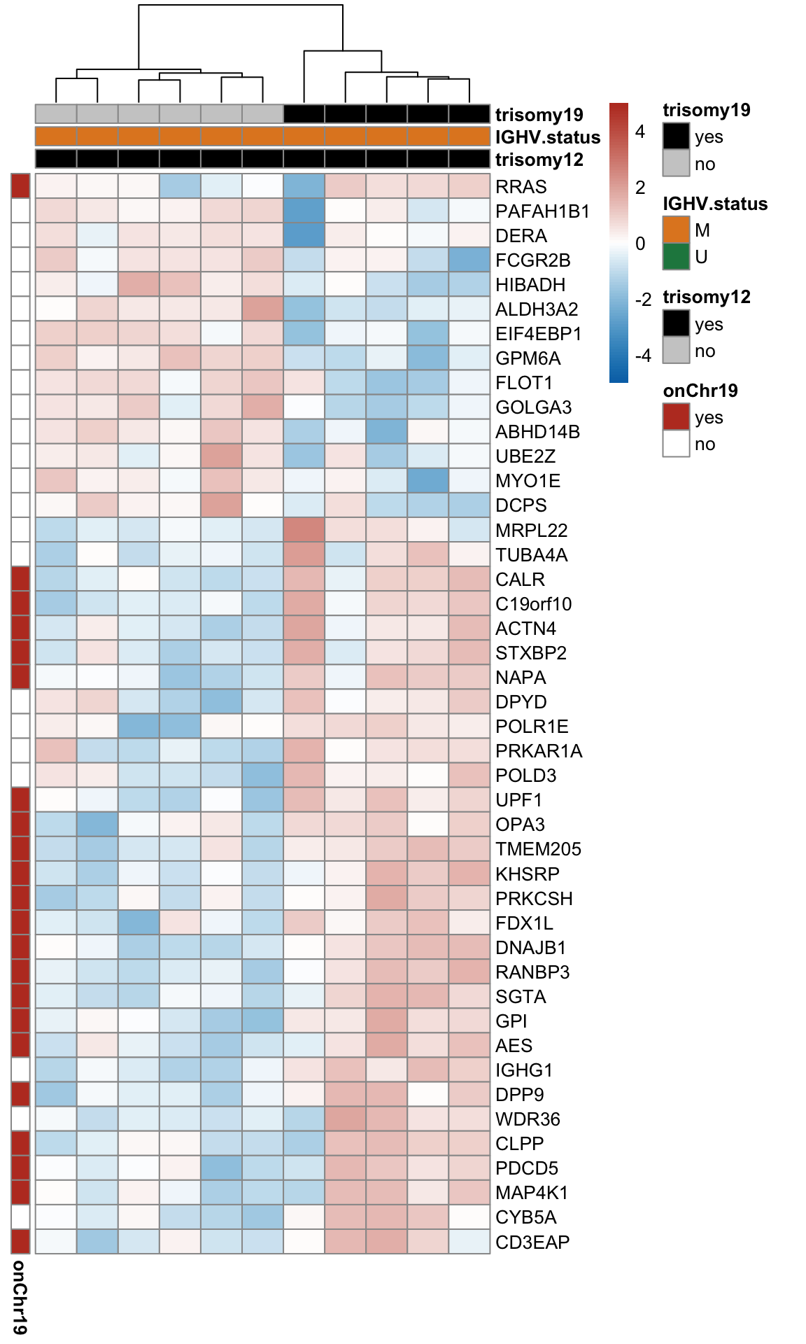
Proteins/RNAs on Chr19 have higher expressions in trisomy19 samples compared to other samples
plotTab <- filter(comExprTab, ChromID %in% "chr19") %>%
  group_by(id,type) %>% mutate(med=mean(expr)) %>% mutate(expr = (expr-med)) %>%
  group_by(id, symbol, cnv, type) %>% summarise(meanExpr = mean(expr, na.rm=TRUE)) %>%
  ungroup()

ggplot(plotTab, aes(x=meanExpr, fill = cnv, col=cnv)) +
  geom_histogram(position = "identity", alpha=0.5) + facet_wrap(~type, scale = "free") +
  scale_fill_manual(values = c(WT = "grey80", trisomy19 = colList[1]), name = "") +
  scale_color_manual(values = c(WT = "grey80", trisomy19 = colList[1]), name = "") +
  theme_full + xlab("Deviation to mean expression")

The variation of expression is higher in RNA than protein
(Maybe figures for supplement) #### For proteins/RNA on chr19
plotTab <- filter(comExprTab, ChromID %in% "chr19") %>%
  group_by(id, symbol, type) %>% summarise(varExp = sd(expr, na.rm=TRUE)) %>%
  ungroup()

ggplot(plotTab, aes(x=varExp,  fill = type, col=type)) +
  geom_histogram(position = "identity", alpha=0.5) +
  scale_fill_manual(values = c(RNA = colList[4], Protein = colList[5]), name = "") +
  scale_color_manual(values = c(RNA = colList[4], Protein = colList[5]), name = "") +
  theme_full + xlab("Standard deviation of expression")

The same trend can be oberserved for non-chr12 proteins/RNAs, but less striking
plotTab <- filter(comExprTab, !ChromID %in% "chr19") %>%
  group_by(id, symbol, type) %>% summarise(varExp = sd(expr, na.rm=TRUE)) %>%
  ungroup()

ggplot(plotTab, aes(x=varExp, fill = type, col=type)) +
  geom_histogram(position = "identity", alpha=0.5) +
  scale_fill_manual(values = c(RNA = colList[4], Protein = colList[5]), name = "") +
  scale_color_manual(values = c(RNA = colList[4], Protein = colList[5]), name = "") +
  theme_full + xlab("Standard deviation of expression")

The overall scale of change is higher in RNA expression than protein expression
(Maybe for supplement)
plotTab <- filter(comExprTab, ChromID %in% "chr19") %>%
  group_by(id, symbol, type, cnv) %>% summarise(meanExp = mean(expr, na.rm=TRUE)) %>%
  ungroup() %>% spread(key = cnv, value = meanExp) %>%
  mutate(log2FC = log2(trisomy19/WT))

ggplot(plotTab, aes(x=log2FC, fill = type, col=type)) +
  geom_histogram(position = "identity", alpha=0.5, bins = 100) +
  scale_fill_manual(values = c(RNA = colList[3], Protein = colList[4]), name = "") +
  scale_color_manual(values = c(RNA = colList[3], Protein = colList[4]), name = "") +
  coord_cartesian(xlim=c(-0.25,0.25))+
  geom_vline(xintercept = 0, col = colList[1], linetype = "dashed") +
  theme_full + xlab("log2 Fold Change")

Analyzing buffering effect
Detect buffered and non-buffered proteins
Preprocessing protein and RNA data
#subset samples and genes
overSampe <- intersect(colnames(ddsCLL), colnames(protCLL))
overGene <- intersect(rownames(ddsCLL), rowData(protCLL)$ensembl_gene_id)
ddsSub <- ddsCLL[overGene, overSampe]
protSub <- protCLL[match(overGene, rowData(protCLL)$ensembl_gene_id),overSampe]
rowData(ddsSub)$uniprotID <- rownames(protSub)[match(rownames(ddsSub),rowData(protSub)$ensembl_gene_id)]

#vst
ddsSub.vst <- varianceStabilizingTransformation(ddsSub)
Differential expression on RNA level
design(ddsSub) <- ~ IGHV + trisomy12 + trisomy19
deRes <- DESeq(ddsSub, betaPrior = TRUE)
rnaRes <- results(deRes, name = "trisomy191", tidy = TRUE) %>%
  dplyr::rename(geneID = row, log2FC.rna = log2FoldChange,
                pvalue.rna = pvalue, padj.rna = padj, stat.rna= stat) %>%
  select(geneID, log2FC.rna, pvalue.rna, padj.rna, stat.rna)
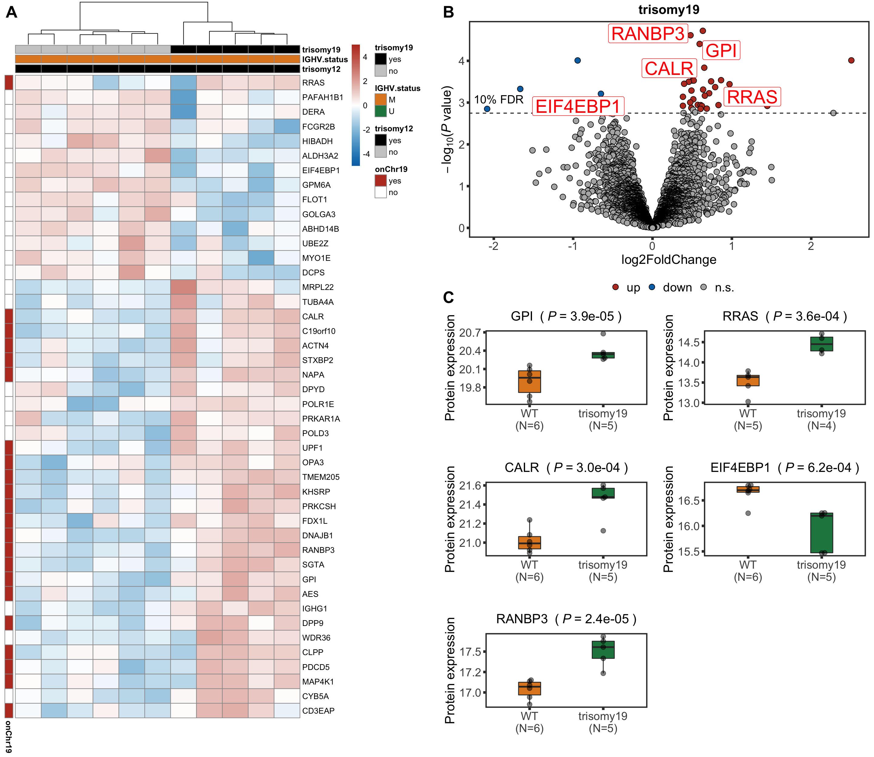
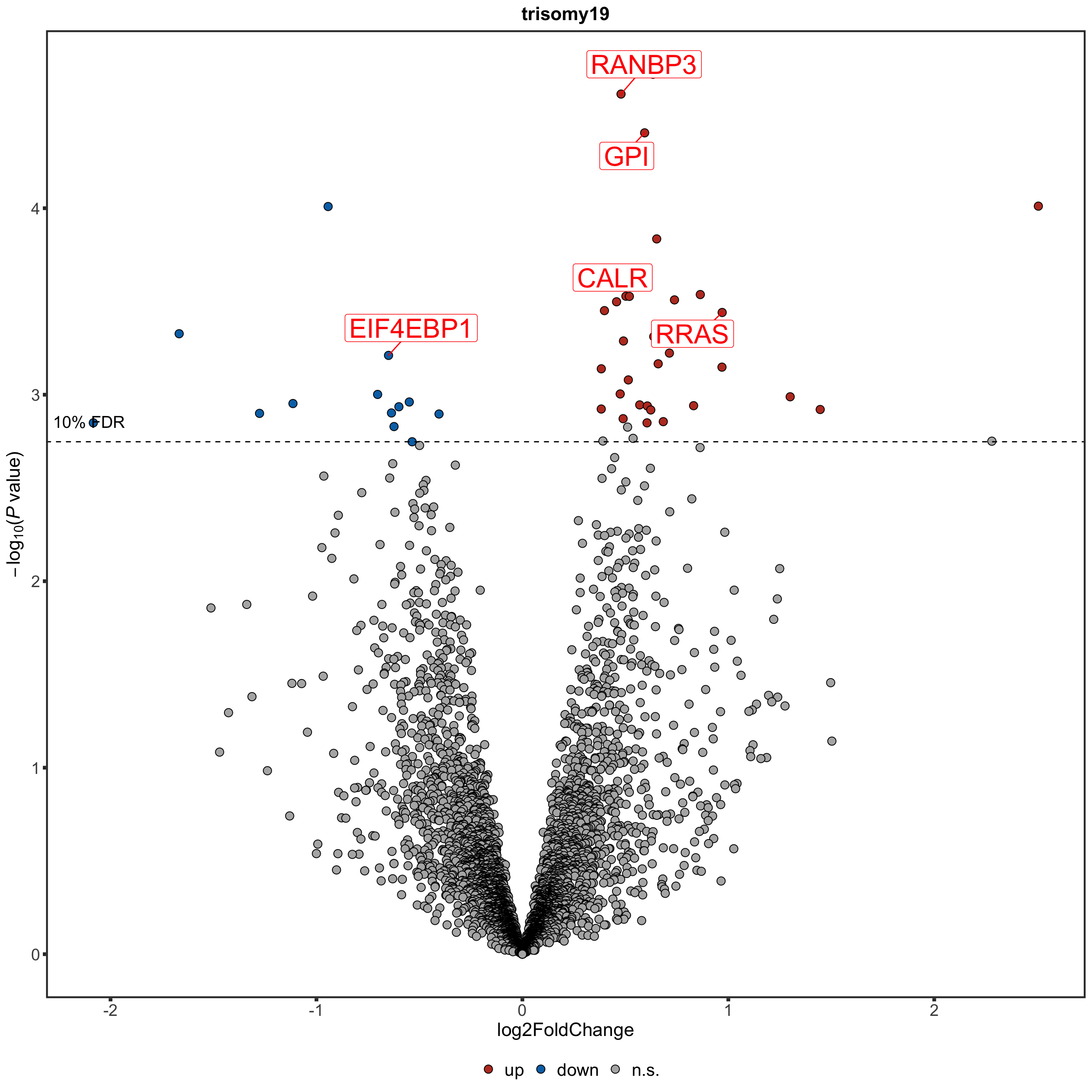
Protein abundance changes related to trisomy19
fdrCut <- 0.1
protRes <- resList %>% filter(Gene == "trisomy19") %>%
    dplyr::rename(uniprotID = id,
                  pvalue = P.Value, padj = adj.P.IHW,
                  chrom = Chr) %>%
    mutate(geneID = rowData(protCLL[uniprotID,])$ensembl_gene_id) %>%
    select(name, uniprotID, geneID, chrom, logFC, pvalue, padj, t) %>%
    dplyr::rename(stat =t) %>%
    arrange(pvalue) %>% as_tibble()
Combine
allRes <- left_join(protRes, rnaRes, by = "geneID")
Only chr19 genes that are up-regulated are considered. Otherwise it's hard to intepret the dosage effect.
bufferTab <- allRes %>% filter(chrom %in% 19,stat.rna > 0) %>%
  ungroup() %>%
  mutate(stat.prot.sqrt = sqrt(stat),
         stat.prot.center = stat.prot.sqrt - mean(stat.prot.sqrt)) %>%
  mutate(score = -stat.prot.center*stat.rna) %>%
  mutate(ifBuffer = case_when(
    padj < 0.1 & padj.rna < 0.1 & stat > 0 ~ "non-Buffered",
    padj > 0.1 & padj.rna < 0.1 ~ "Buffered",
    padj < 0.1 & padj.rna > 0.1 & stat > 0 ~ "Enhanced",
    TRUE ~ "Undetermined"
  )) %>%
  arrange(desc(score))
Table of buffering status
bufferTab %>% mutate_if(is.numeric, formatC, digits=2) %>%
  select(name, pvalue, pvalue.rna, padj, padj.rna, ifBuffer) %>%
  DT::datatable()
Summary plot
sumTab <- bufferTab %>% group_by(ifBuffer) %>%
  summarise(n = length(name))

ggplot(sumTab, aes(x=ifBuffer, y = n)) +
  geom_bar(aes(fill = ifBuffer), stat="identity") +
  geom_text(aes(label = paste0("n=", n)),vjust=-1,col=colList[1]) +
  scale_fill_manual(values =c(Buffered = colList[1],
                              Enhanced = colList[4],
                              `non-Buffered` = colList[2],
                              Undetermined = "grey50")) +
  theme_half + theme(axis.text.x = element_text(angle = 90, hjust=1, vjust=0.5),
                     legend.position = "none") +
  ylab("Number of proteins") + ylim(0,130)

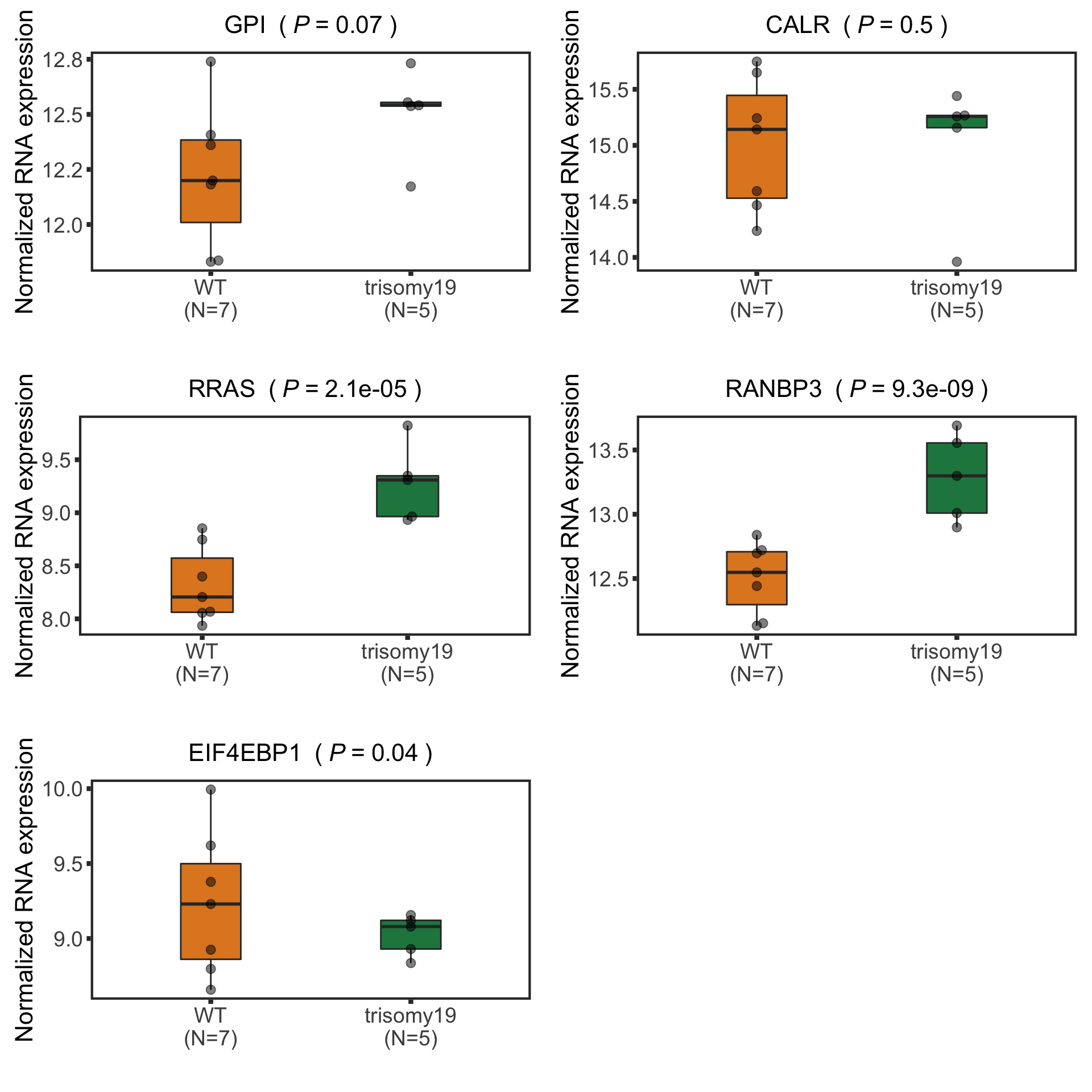
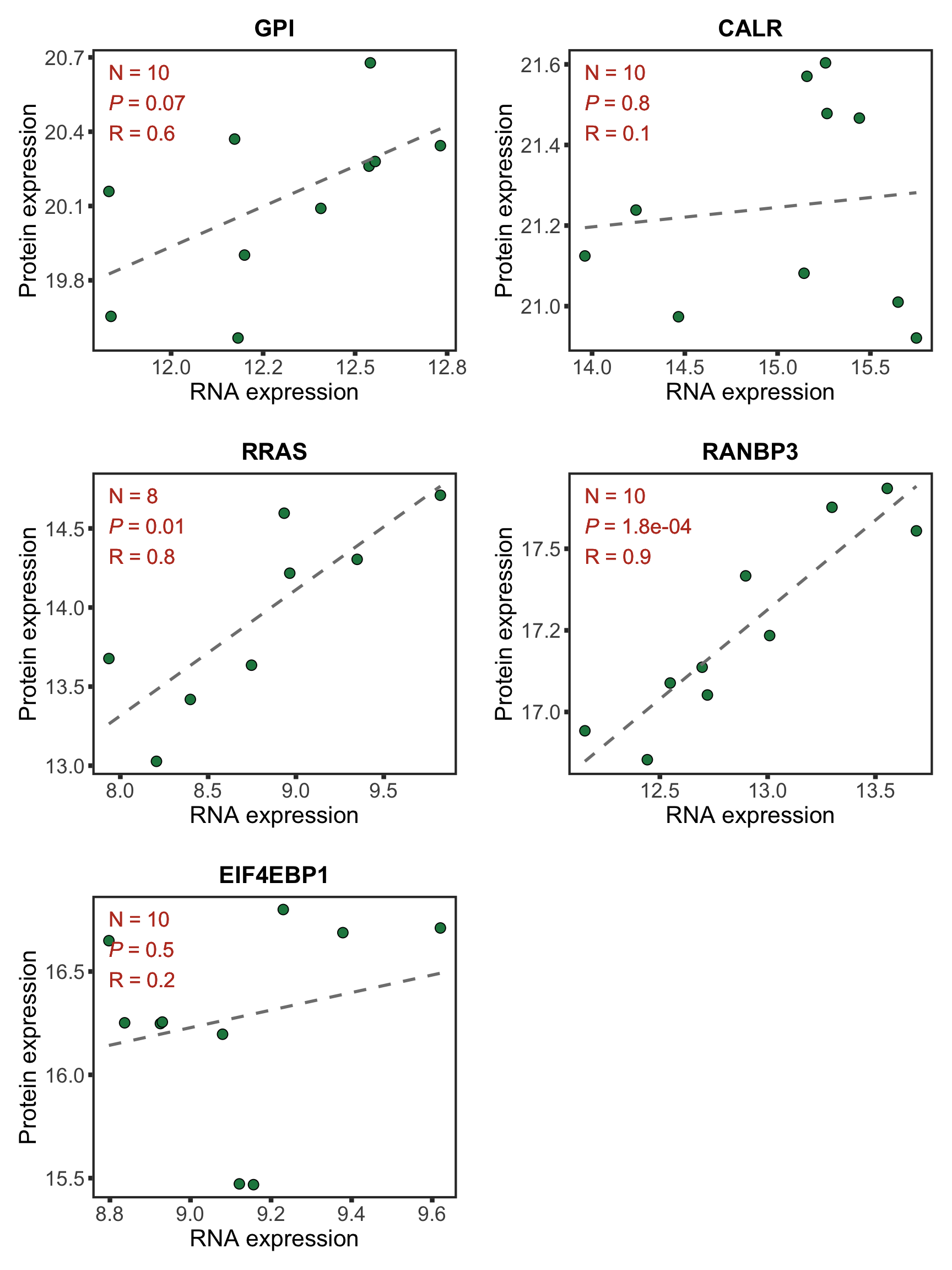
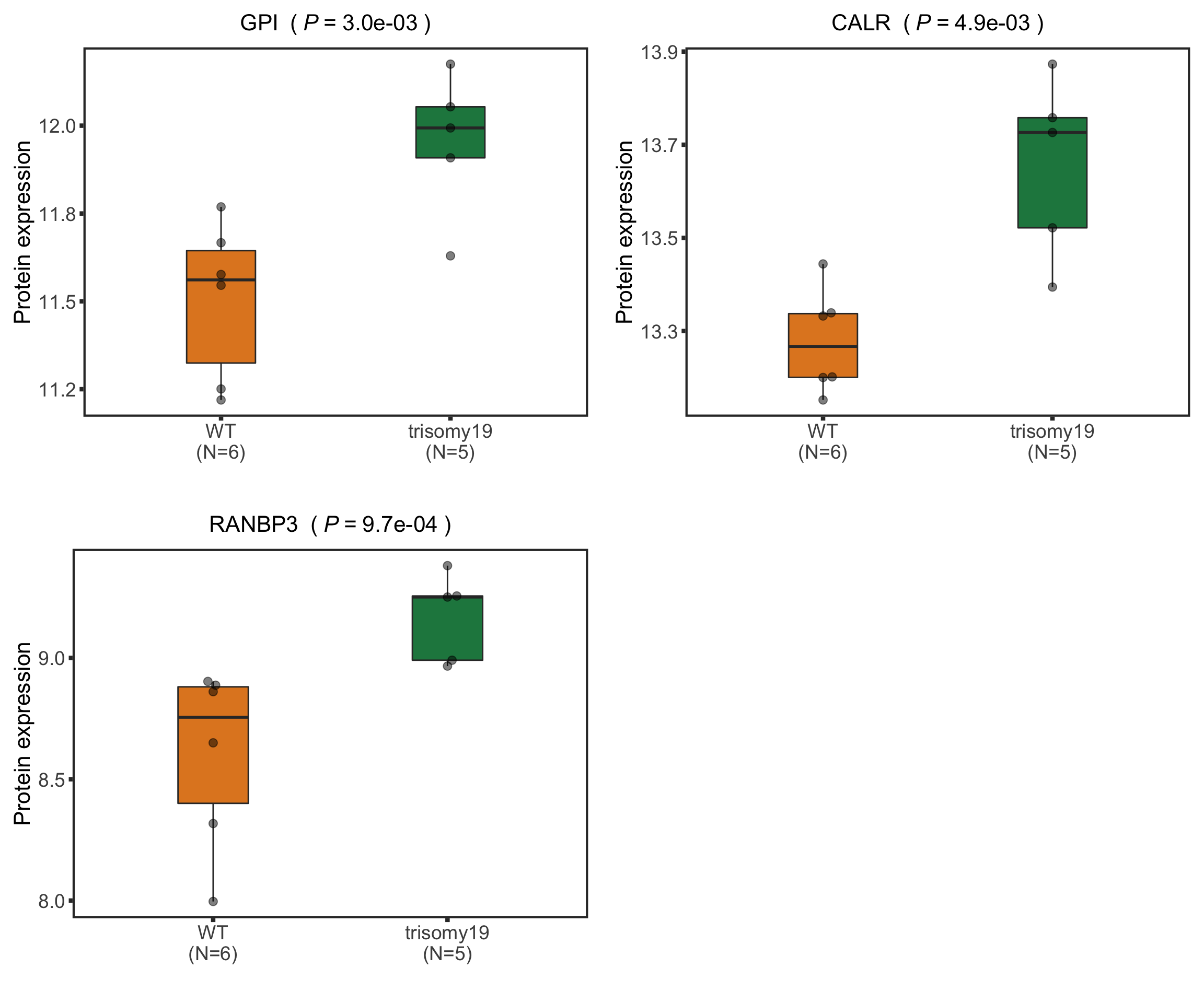
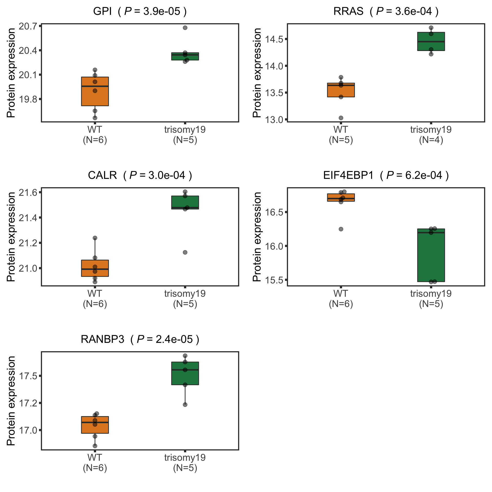
Plot example cases of buffered and non-buffered proteins
protList <- c("RRAS","ERCC2","NACC1", "MAP4K1")
geneList <- bufferTab[match(protList, bufferTab$name),]$geneID
pList <- lapply(geneList, function(i) {
  tabProt <- allProtTab %>% filter(id == i) %>%
    select(id, patID, symbol,expr) %>% dplyr::rename(protExpr = expr)
  tabRna <- allRnaTab %>% filter(id == i) %>%
    select(id, patID, expr) %>% dplyr::rename(rnaExpr = expr)
  plotTab <- left_join(tabProt, tabRna, by = c("id","patID")) %>%
    filter(!is.na(protExpr), !is.na(rnaExpr)) %>%
    mutate(trisomy19 = patMeta[match(patID, patMeta$Patient.ID),]$trisomy19,
           trisomy12 = patMeta[match(patID, patMeta$Patient.ID),]$trisomy12,
           IGHV = patMeta[match(patID, patMeta$Patient.ID),]$IGHV.status) %>%
    filter(!is.na(trisomy19),trisomy12 %in% 1, IGHV %in%"M") %>%
    mutate(trisomy19 = ifelse(trisomy19 %in% 1, "yes","no"))
  p <- ggplot(plotTab, aes(x=rnaExpr, y = protExpr)) +
    geom_point(aes(col=trisomy19)) +
    geom_smooth(formula =  y~x, method="lm",se=FALSE, color = "grey50", linetype ="dashed" ) +
    ggtitle(unique(plotTab$symbol)) +
    ylab("Protein expression") + xlab("RNA expression") +
    scale_color_manual(values =c(yes = colList[1],no=colList[2])) +
    theme_full + theme(legend.position = "bottom")
  ggExtra::ggMarginal(p, type = "histogram", groupFill = TRUE)
  })
cowplot::plot_grid(plotlist = pList, ncol=2)
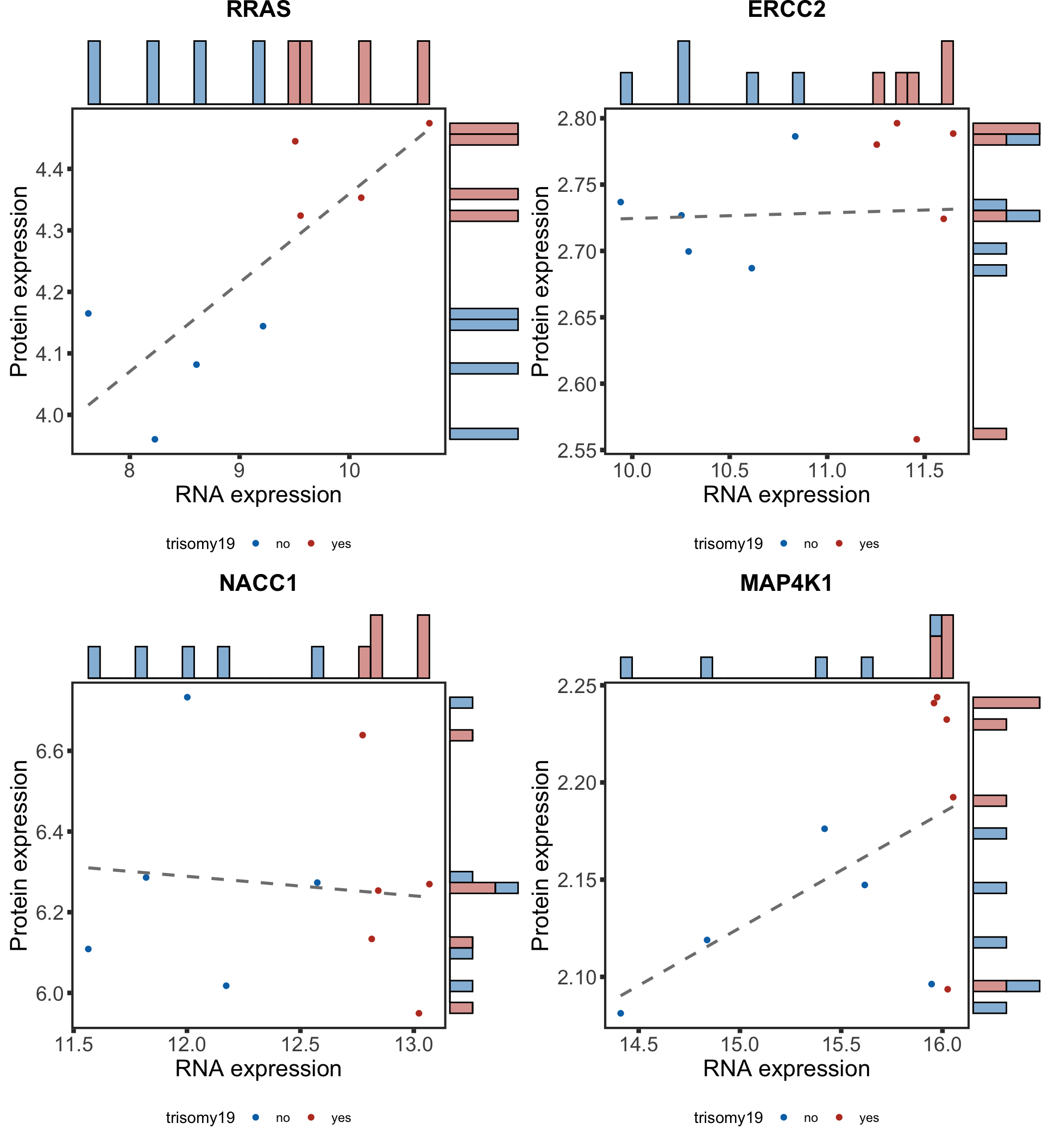 FDX2 is a protein that can not be uniquely mapped and therefore removed from the analysis. We can choose other buffered proteins as examples
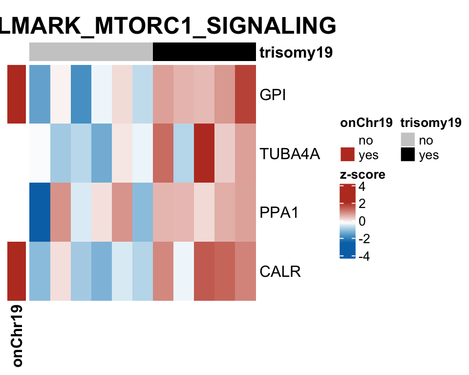
Enrichment of buffer and non-buffered proteins
Non-buffered prpteins
protList <- filter(bufferTab, ifBuffer == "non-Buffered")$name
refList <- unique(protExprTab$symbol)
enRes <- runFisher(protList, refList, gmts$H, pCut =0.05, ifFDR = FALSE)
[1] "No sets passed the criteria"
enRes$enrichPlot
NULL
Buffered proteins
protList <- filter(bufferTab, ifBuffer == "Buffered")$name
enRes <- runFisher(protList, refList, gmts$H, pCut =0.05, ifFDR = FALSE)
[1] "No sets passed the criteria"
Enhanced proteins
protList <- filter(bufferTab, ifBuffer == "Enhanced")$name
enRes <- runFisher(protList, refList, gmts$H, pCut =0.05, ifFDR = FALSE)
[1] "No sets passed the criteria"
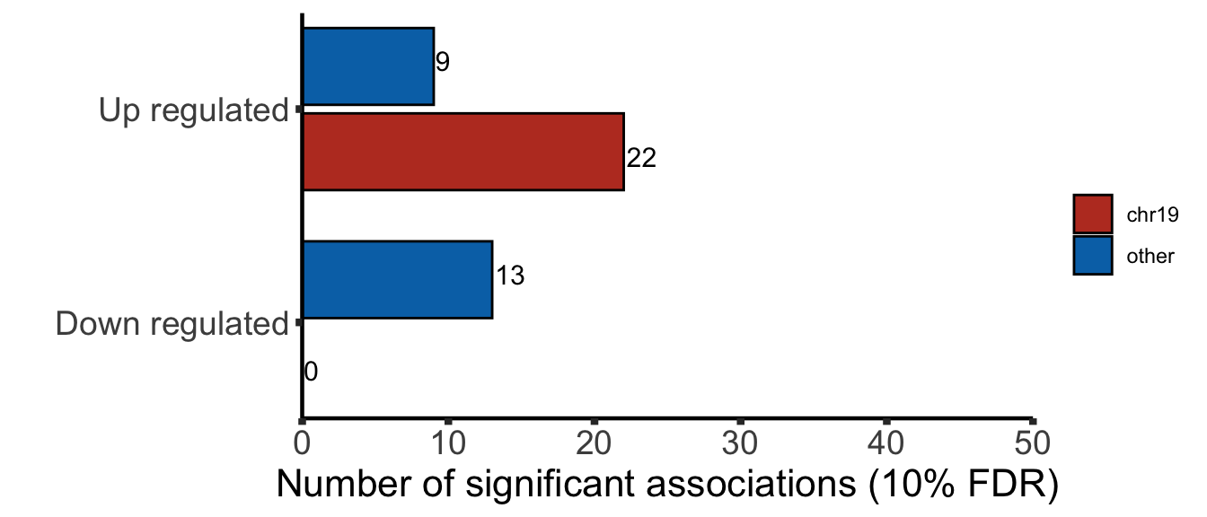
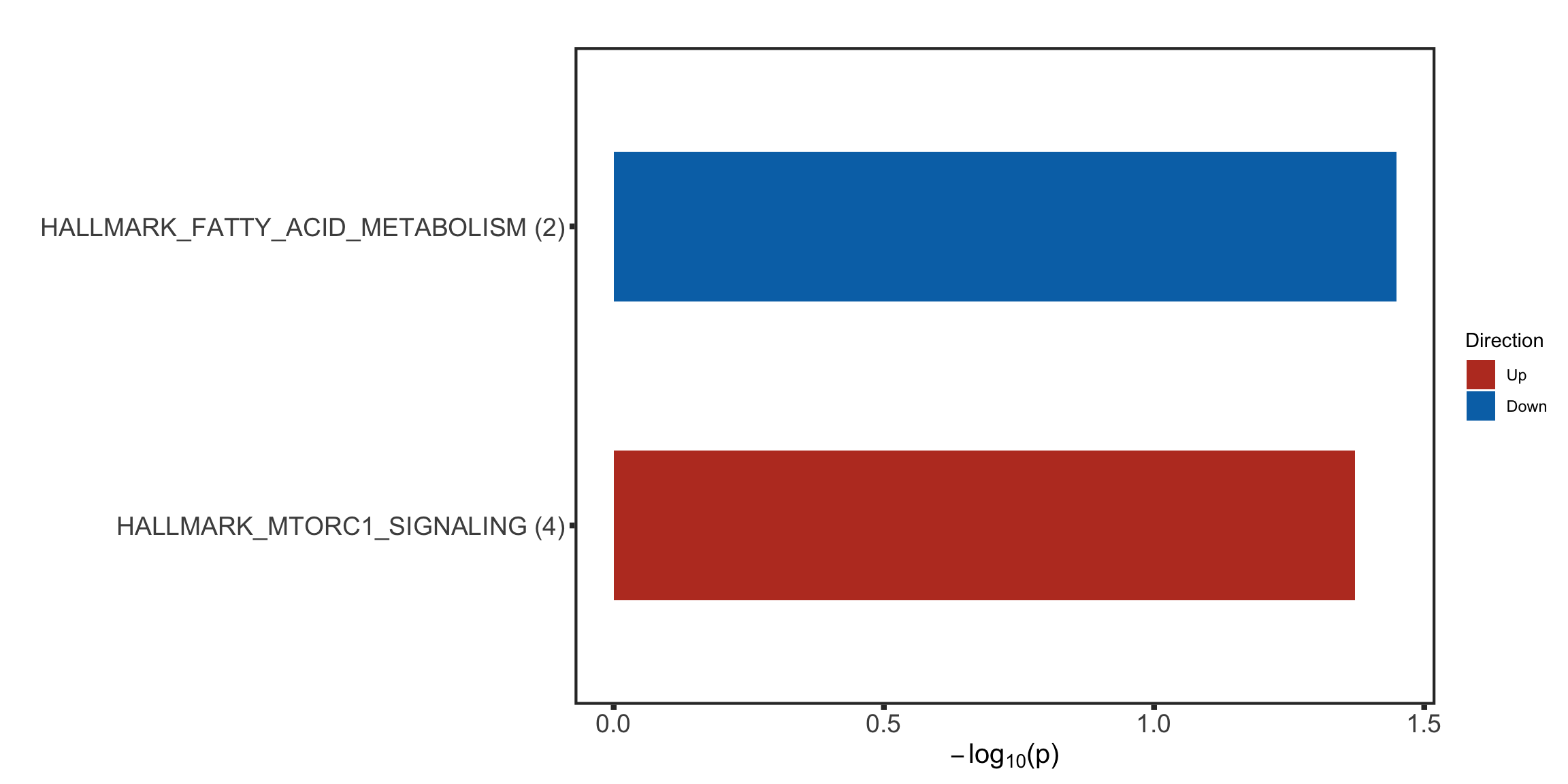 Note that none of the pathways passed 10% FDR