Last updated: 2020-10-20

Checks: 5 2

Knit directory: Proteomics/analysis/

This reproducible R Markdown analysis was created with workflowr (version 1.6.2). The Checks tab describes the reproducibility checks that were applied when the results were created. The Past versions tab lists the development history.


The R Markdown is untracked by Git. To know which version of the R Markdown file created these results, you'll want to first commit it to the Git repo. If you're still working on the analysis, you can ignore this warning. When you're finished, you can run wflow_publish to commit the R Markdown file and build the HTML.

Great job! The global environment was empty. Objects defined in the global environment can affect the analysis in your R Markdown file in unknown ways. For reproduciblity it's best to always run the code in an empty environment.

The command set.seed(20200227) was run prior to running the code in the R Markdown file. Setting a seed ensures that any results that rely on randomness, e.g. subsampling or permutations, are reproducible.

Great job! Recording the operating system, R version, and package versions is critical for reproducibility.

The following chunks had caches available:
  • unnamed-chunk-10
  • unnamed-chunk-18
  • unnamed-chunk-21

To ensure reproducibility of the results, delete the cache directory manuscript_S8_drugResponse_Outcomes_cache and re-run the analysis. To have workflowr automatically delete the cache directory prior to building the file, set delete_cache = TRUE when running wflow_build() or wflow_publish().

Great job! Using relative paths to the files within your workflowr project makes it easier to run your code on other machines.

Great! You are using Git for version control. Tracking code development and connecting the code version to the results is critical for reproducibility.

The results in this page were generated with repository version 3fb50c5. See the Past versions tab to see a history of the changes made to the R Markdown and HTML files.

Note that you need to be careful to ensure that all relevant files for the analysis have been committed to Git prior to generating the results (you can use wflow_publish or wflow_git_commit). workflowr only checks the R Markdown file, but you know if there are other scripts or data files that it depends on. Below is the status of the Git repository when the results were generated:


Ignored files:
    Ignored:    .DS_Store
    Ignored:    .Rhistory
    Ignored:    .Rproj.user/
    Ignored:    analysis/.DS_Store
    Ignored:    analysis/.Rhistory
    Ignored:    analysis/correlateCLLPD_cache/
    Ignored:    analysis/lassoForSTAT2_cache/
    Ignored:    analysis/manuscript_S1_Overview_cache/
    Ignored:    analysis/manuscript_S2_genomicAssociation_oldTimsTOF_cache/
    Ignored:    analysis/manuscript_S3_trisomy12_cache/
    Ignored:    analysis/manuscript_S4_IGHV_cache/
    Ignored:    analysis/manuscript_S4_IGHV_oldTimsTOF_cache/
    Ignored:    analysis/manuscript_S5_trisomy19_cache/
    Ignored:    analysis/manuscript_S6_del11q_cache/
    Ignored:    analysis/manuscript_S6_del11q_oldTimsTOF_cache/
    Ignored:    analysis/manuscript_S7_SF3B1_cache/
    Ignored:    analysis/manuscript_S8_drugResponse_Outcomes_cache/
    Ignored:    analysis/manuscript_S9_STAT2_cache/
    Ignored:    code/.Rhistory
    Ignored:    data/.DS_Store
    Ignored:    output/.DS_Store

Untracked files:
    Untracked:  analysis/.trisomy12_norm.pdf
    Untracked:  analysis/CNVanalysis_11q.Rmd
    Untracked:  analysis/CNVanalysis_trisomy12.Rmd
    Untracked:  analysis/CNVanalysis_trisomy19.Rmd
    Untracked:  analysis/STAT2_cytokines.Rmd
    Untracked:  analysis/SUGP1_splicing.svg.xml
    Untracked:  analysis/analysisDrugResponses.Rmd
    Untracked:  analysis/analysisDrugResponses_IC50.Rmd
    Untracked:  analysis/analysisPCA.Rmd
    Untracked:  analysis/analysisPreliminary_LUMOS.Rmd
    Untracked:  analysis/analysisPreliminary_timsTOF_Hela.Rmd
    Untracked:  analysis/analysisPreliminary_timsTOF_new.Rmd
    Untracked:  analysis/analysisSplicing.Rmd
    Untracked:  analysis/analysisTrisomy19.Rmd
    Untracked:  analysis/annotateCNV.Rmd
    Untracked:  analysis/comparePlatforms_LUMOS_helaTimsTOF.Rmd
    Untracked:  analysis/comparePlatforms_LUMOS_newTimsTOF.Rmd
    Untracked:  analysis/comparePlatforms_newTimsTOF_helaTimsTOF.Rmd
    Untracked:  analysis/complexAnalysis_IGHV.Rmd
    Untracked:  analysis/complexAnalysis_IGHV_alternative.Rmd
    Untracked:  analysis/complexAnalysis_overall.Rmd
    Untracked:  analysis/complexAnalysis_trisomy12.Rmd
    Untracked:  analysis/complexAnalysis_trisomy12_alternative.Rmd
    Untracked:  analysis/correlateGenomic_PC12adjusted.Rmd
    Untracked:  analysis/correlateGenomic_noBlock.Rmd
    Untracked:  analysis/correlateGenomic_noBlock_MCLL.Rmd
    Untracked:  analysis/correlateGenomic_noBlock_UCLL.Rmd
    Untracked:  analysis/correlateGenomic_timsTOFnew.Rmd
    Untracked:  analysis/correlateGenomic_timsTOFnewHela.Rmd
    Untracked:  analysis/correlateRNAexpression.Rmd
    Untracked:  analysis/default.css
    Untracked:  analysis/del11q.pdf
    Untracked:  analysis/del11q_norm.pdf
    Untracked:  analysis/full_diff_list.csv
    Untracked:  analysis/lassoForSTAT2.Rmd
    Untracked:  analysis/manuscript_S0_PrepareData.Rmd
    Untracked:  analysis/manuscript_S1_Overview.Rmd
    Untracked:  analysis/manuscript_S2_genomicAssociation.Rmd
    Untracked:  analysis/manuscript_S2_genomicAssociation_oldTimsTOF.Rmd
    Untracked:  analysis/manuscript_S3_trisomy12.Rmd
    Untracked:  analysis/manuscript_S4_IGHV.Rmd
    Untracked:  analysis/manuscript_S4_IGHV_oldTimsTOF.Rmd
    Untracked:  analysis/manuscript_S5_trisomy19.Rmd
    Untracked:  analysis/manuscript_S6_del11q.Rmd
    Untracked:  analysis/manuscript_S6_del11q_oldTimsTOF.Rmd
    Untracked:  analysis/manuscript_S7_SF3B1.Rmd
    Untracked:  analysis/manuscript_S8_drugResponse_Outcomes.Rmd
    Untracked:  analysis/manuscript_S9_STAT2.Rmd
    Untracked:  analysis/peptideValidate.Rmd
    Untracked:  analysis/plotCNV_del11q.pdf
    Untracked:  analysis/plotExpressionCNV.Rmd
    Untracked:  analysis/processPeptides_LUMOS.Rmd
    Untracked:  analysis/processProteomics_timsTOF_Hela.Rmd
    Untracked:  analysis/processProteomics_timsTOF_new.Rmd
    Untracked:  analysis/protCLL.RData
    Untracked:  analysis/qualityControl_timsTOF_Hela.Rmd
    Untracked:  analysis/qualityControl_timsTOF_new.Rmd
    Untracked:  analysis/style.css
    Untracked:  analysis/tableS1_DE_proteins_p0.01.xlsx
    Untracked:  analysis/test.pdf
    Untracked:  analysis/test.svg
    Untracked:  analysis/tri12Enrich.pdf
    Untracked:  analysis/trisomy12.pdf
    Untracked:  analysis/trisomy12_AFcor.Rmd
    Untracked:  analysis/trisomy12_norm.pdf
    Untracked:  code/AlteredPQR.R
    Untracked:  code/utils.R
    Untracked:  data/190909_CLL_prot_abund_med_norm.tsv
    Untracked:  data/190909_CLL_prot_abund_no_norm.tsv
    Untracked:  data/200725_cll_diaPASEF_direct_reports/
    Untracked:  data/200728_cll_diaPASEF_direct_plus_hela_reports/
    Untracked:  data/20190423_Proteom_submitted_samples_bereinigt.xlsx
    Untracked:  data/20191025_Proteom_submitted_samples_final.xlsx
    Untracked:  data/Chemokines.csv
    Untracked:  data/IFN_list.csv
    Untracked:  data/IFNreceptor.csv
    Untracked:  data/Interleukin_receptor.csv
    Untracked:  data/Interleukins.csv
    Untracked:  data/LUMOS/
    Untracked:  data/LUMOS_peptides/
    Untracked:  data/LUMOS_protAnnotation.csv
    Untracked:  data/LUMOS_protAnnotation_fix.csv
    Untracked:  data/SampleAnnotation_cleaned.xlsx
    Untracked:  data/chemoReceptor.csv
    Untracked:  data/example_proteomics_data
    Untracked:  data/facTab_IC50atLeast3New.RData
    Untracked:  data/gmts/
    Untracked:  data/mapEnsemble.txt
    Untracked:  data/mapSymbol.txt
    Untracked:  data/proteins_in_complexes
    Untracked:  data/pyprophet_export_aligned.csv
    Untracked:  data/timsTOF_protAnnotation.csv
    Untracked:  output/Fig1A.pdf
    Untracked:  output/Fig1A.png
    Untracked:  output/Fig1A.pptx
    Untracked:  output/LUMOS_processed.RData
    Untracked:  output/MSH6_splicing.svg
    Untracked:  output/SUGP1_splicing.eps
    Untracked:  output/SUGP1_splicing.pdf
    Untracked:  output/SUGP1_splicing.svg
    Untracked:  output/cnv_plots.zip
    Untracked:  output/cnv_plots/
    Untracked:  output/cnv_plots_norm.zip
    Untracked:  output/ddsrna_enc.RData
    Untracked:  output/deResList.RData
    Untracked:  output/deResList_timsTOF.RData
    Untracked:  output/deResList_timsTOF_old.RData
    Untracked:  output/dxdCLL.RData
    Untracked:  output/dxdCLL2.RData
    Untracked:  output/encMap.RData
    Untracked:  output/exprCNV.RData
    Untracked:  output/exprCNV_enc.RData
    Untracked:  output/lassoResults_CPS.RData
    Untracked:  output/lassoResults_IC50.RData
    Untracked:  output/patMeta_enc.RData
    Untracked:  output/pepCLL_lumos.RData
    Untracked:  output/pepCLL_lumos_enc.RData
    Untracked:  output/pepTab_lumos.RData
    Untracked:  output/pheno1000_enc.RData
    Untracked:  output/pheno1000_main.RData
    Untracked:  output/plotCNV_allChr11_diff.pdf
    Untracked:  output/plotCNV_del11q_sum.pdf
    Untracked:  output/proteomic_LUMOS_20200227.RData
    Untracked:  output/proteomic_LUMOS_20200320.RData
    Untracked:  output/proteomic_LUMOS_20200430.RData
    Untracked:  output/proteomic_LUMOS_enc.RData
    Untracked:  output/proteomic_timsTOF_20200227.RData
    Untracked:  output/proteomic_timsTOF_Hela_20200806.RData
    Untracked:  output/proteomic_timsTOF_enc.RData
    Untracked:  output/proteomic_timsTOF_new_20200806.RData
    Untracked:  output/proteomic_timsTOF_old_enc.RData
    Untracked:  output/splicingResults.RData
    Untracked:  output/survival_enc.RData
    Untracked:  output/timsTOF_processed.RData
    Untracked:  plotCNV_del11q_diff.pdf
    Untracked:  summary/
    Untracked:  supp_latex/

Unstaged changes:
    Modified:   analysis/_site.yml
    Modified:   analysis/analysisSF3B1.Rmd
    Modified:   analysis/compareProteomicsRNAseq.Rmd
    Modified:   analysis/correlateCLLPD.Rmd
    Modified:   analysis/correlateGenomic.Rmd
    Deleted:    analysis/correlateGenomic_removePC.Rmd
    Modified:   analysis/correlateMIR.Rmd
    Modified:   analysis/correlateMethylationCluster.Rmd
    Modified:   analysis/index.Rmd
    Modified:   analysis/predictOutcome.Rmd
    Modified:   analysis/processProteomics_LUMOS.Rmd
    Modified:   analysis/qualityControl_LUMOS.Rmd

Note that any generated files, e.g. HTML, png, CSS, etc., are not included in this status report because it is ok for generated content to have uncommitted changes.


There are no past versions. Publish this analysis with wflow_publish() to start tracking its development.


Correlations between protein abundance and drug response

Preprocess datasets

Drug screening data from 1000CPS: low quality samples after QC are removed; the edge effect corrected viability values are used

viabMat <- pheno1000_main %>% filter(!lowQuality, ! Drug %in% c("DMSO","PBS"), patientID %in% colnames(protCLL)) %>%
  group_by(patientID, Drug) %>% summarise(viab = mean(normVal.adj.cor_auc)) %>%
  spread(key = patientID, value = viab) %>%
  data.frame(stringsAsFactors = FALSE) %>% column_to_rownames("Drug") %>%
  as.matrix()

Proteomics data

proMat <- assays(protCLL)[["count"]]
proMat <- proMat[,colnames(viabMat)]

#Remove proteins without much variance (to lower multi-testing burden)

sds <- genefilter::rowSds(proMat,na.rm=TRUE)
proMat <- proMat[sds > genefilter::shorth(sds),]

How many samples have both proteomics data and CPS1000 screen data

ncol(proMat)
[1] 45

Association test

resTab.auc <- lapply(rownames(viabMat),function(drugName) {
  viab <- viabMat[drugName, ]
  designMat <- model.matrix(~1+viab)
  fit <- lmFit(proMat,  designMat)
  fit2 <- eBayes(fit)
  corRes <- topTable(fit2, number ="all", adjust.method = "BH", coef = "viab") %>% rownames_to_column("id") %>%
    mutate(symbol = rowData(protCLL[id,])$hgnc_symbol, Drug = drugName)
}) %>% bind_rows() %>% mutate(adj.P.Val = p.adjust(P.Value, method = "BH")) %>% arrange(P.Value)

Bar plot to show the number of associations (10% FDR)

#Select significant associations (10% FDR)
resTab.sig <- filter(resTab.auc, adj.P.Val < 0.1) %>% 
  select(Drug, symbol, id,logFC, P.Value, adj.P.Val)

plotTab <- resTab.sig %>% group_by(Drug) %>%
  summarise(n = length(id)) %>% ungroup()
ordTab <- group_by(plotTab, Drug) %>% summarise(total = sum(n)) %>%
  arrange(desc(total))
plotTab <- mutate(plotTab, Drug = factor(Drug, levels = ordTab$Drug)) %>%
  filter(n>0)

drugBar <- ggplot(plotTab, aes(x=Drug, y = n)) + geom_bar(stat="identity",fill=colList[4]) + 
  geom_text(aes(label = paste0("n=", n)),vjust=-1,col=colList[1]) +
  ylim(0,15)+ annotate("text", label = "Number of associations (10% FDR)", x=Inf, y=Inf,hjust=1, vjust=1.5, size=6)+
  theme_half + theme(axis.text.x = element_text(angle = 90, hjust=1, vjust=0.5)) +
  ylab("Number") + xlab("")

drugBar

Table of significant associations (10% FDR)

resTab.sig %>% mutate_if(is.numeric, formatC, digits=2, format= "e") %>%
  DT::datatable()

Correlation plot of selected candidates

plotDrugCorScatter <- function(inputTab, x, y, x_lab = "X", y_lab = "Y", title = "",
                           col = NULL, showR2 = TRUE, annoPos = "right",
                           dotCol = colList, textCol="darkred") {

  #prepare table for plotting
  plotTab <- tibble(x = inputTab[[x]],y=inputTab[[y]])
  if (!is.null(col)) plotTab <- mutate(plotTab, status = inputTab[[col]])
  plotTab <- filter(plotTab, !is.na(x), !is.na(y))

  #prepare annotation values
  corRes <- cor.test(plotTab$x, plotTab$y)
  pval <- formatNum(corRes$p.value, digits = 1, format = "e")
  Rval <- formatNum(corRes$estimate, digits = 1, format = "e")
  R2val <- formatNum(corRes$estimate^2, digits = 1, format = "e")
  Nval <- nrow(plotTab)
  annoP <- bquote(italic("P")~"="~.(pval))

  if (showR2) {
    annoCoef <-  bquote(R^2~"="~.(R2val))
  } else {
    annoCoef <- bquote(R~"="~.(Rval))
  }
  annoN <- bquote(N~"="~.(Nval))

  corPlot <- ggplot(plotTab, aes(x = x, y = y))

  if (!is.null(col)) {
    corPlot <- corPlot + geom_point(aes(fill = status), shape =21, size =3) +
      scale_fill_manual(values = dotCol)
  } else {
    corPlot <- corPlot + geom_point(fill = dotCol[1], shape =21, size=3)
  }

  corPlot <- corPlot +   geom_smooth(formula = y~x,method = "lm", se=FALSE, color = "grey50", linetype ="dashed" )

  if (annoPos == "right") {

    corPlot <- corPlot + annotate("text", x = max(plotTab$x), y = Inf, label = annoN,
                                  hjust=1, vjust =2, size = 5, parse = FALSE, col= textCol) +
      annotate("text", x = max(plotTab$x), y = Inf, label = annoP,
               hjust=1, vjust =4, size = 5, parse = FALSE, col= textCol) +
      annotate("text", x = max(plotTab$x), y = Inf, label = annoCoef,
               hjust=1, vjust =6, size = 5, parse = FALSE, col= textCol)

  } else if (annoPos== "left") {
    corPlot <- corPlot + annotate("text", x = min(plotTab$x), y = Inf, label = annoN,
                                  hjust=0, vjust =2, size = 5, parse = FALSE, col= textCol) +
      annotate("text", x = min(plotTab$x), y = Inf, label = annoP,
               hjust=0, vjust =4, size = 5, parse = FALSE, col= textCol) +
      annotate("text", x = min(plotTab$x), y = Inf, label = annoCoef,
               hjust=0, vjust =6, size = 5, parse = FALSE, col= textCol)
  }
  corPlot <- corPlot + ylab(y_lab) + xlab(x_lab) + ggtitle(title) +
    scale_y_continuous(labels = scales::number_format(accuracy = 0.1)) +
    scale_x_continuous(labels = scales::number_format(accuracy = 0.1)) +
    theme_full
  corPlot
}
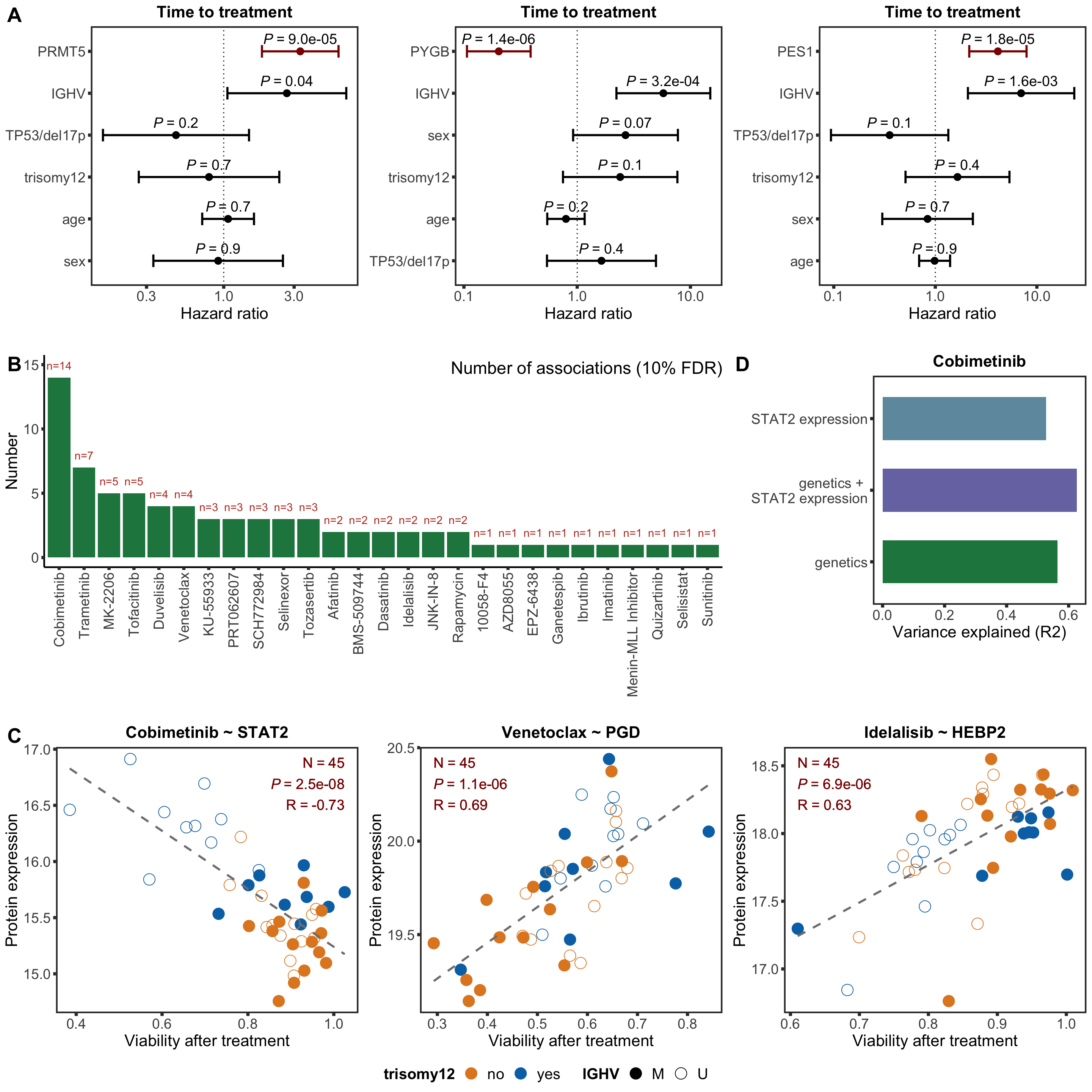
pairList <- list(c("Cobimetinib","STAT2"),c("Venetoclax","PGD"),c("Idelalisib", "HEBP2"))
plotList <- lapply(pairList, function(pair) {
  textCol <- "darkred"
  drugName <- pair[1]
  proteinName <- pair[2]
  id <- rownames(protCLL)[match(proteinName, rowData(protCLL)$hgnc_symbol)]
  plotTab <- tibble(patID = colnames(viabMat), 
                    viab = viabMat[drugName,],
                    expr = proMat[id,]) %>%
    mutate(IGHV = protCLL[,patID]$IGHV.status,
           trisomy12 = protCLL[,patID]$trisomy12) %>%
    mutate(trisomy12 = ifelse(trisomy12 ==1,"yes","no")) %>%
    filter(!is.na(viab),!is.na(expr))
  
  pval <- formatNum(filter(resTab.sig, Drug == drugName, symbol == proteinName)$P.Value, digits = 1, format = "e")
  Rval <- sprintf("%1.2f",cor(plotTab$viab, plotTab$expr))
  Nval <- nrow(plotTab)
  annoP <- bquote(italic("P")~"="~.(pval))
  annoN <- bquote(N~"="~.(Nval))
  annoCoef <- bquote(R~"="~.(Rval))

  corPlot <- ggplot(plotTab, aes(x = viab, y = expr)) + 
    geom_point(aes(col = trisomy12, shape = IGHV), size=5) +
    scale_shape_manual(values = c(M = 19, U = 1)) + 
    scale_color_manual(values = c(yes = colList[2], no = colList[3])) +
    geom_smooth(formula = y~x,method = "lm", se=FALSE, color = "grey50", linetype ="dashed" ) +
    ggtitle(sprintf("%s ~ %s", drugName, proteinName)) +
    ylab("Protein expression") + xlab("Viability after treatment") +
    theme_full +
    theme(legend.position = "bottom", 
          legend.text = element_text(size=15), legend.title = element_text(size=15, face = "bold"))

  if (Rval < 0) annoPos <- "right" else annoPos <- "left"
  
  if (annoPos == "right") {

    corPlot <- corPlot + annotate("text", x = max(plotTab$viab), y = Inf, label = annoN,
                                  hjust=1, vjust =2, size = 5, parse = FALSE, col= textCol) +
      annotate("text", x = max(plotTab$viab), y = Inf, label = annoP,
               hjust=1, vjust =4, size = 5, parse = FALSE, col= textCol) +
      annotate("text", x = max(plotTab$viab), y = Inf, label = annoCoef,
               hjust=1, vjust =6, size = 5, parse = FALSE, col= textCol)

  } else if (annoPos== "left") {
    corPlot <- corPlot + annotate("text", x = min(plotTab$viab), y = Inf, label = annoN,
                                  hjust=0, vjust =2, size = 5, parse = FALSE, col= textCol) +
      annotate("text", x = min(plotTab$viab), y = Inf, label = annoP,
               hjust=0, vjust =4, size = 5, parse = FALSE, col= textCol) +
      annotate("text", x = min(plotTab$viab), y = Inf, label = annoCoef,
               hjust=0, vjust =6, size = 5, parse = FALSE, col= textCol)
  }
  
  corPlot <- corPlot + ylab("Protein expression") + xlab("Viability after treatment") + 
    scale_y_continuous(labels = scales::number_format(accuracy = 0.1)) +
    scale_x_continuous(labels = scales::number_format(accuracy = 0.1))

  corPlot
})

legend <- cowplot::get_legend(plotList[[1]])
plotNoLegend <- lapply(plotList, function(p) p + theme(legend.position  = "none"))
drugCor <- plot_grid(plot_grid(plotlist = plotNoLegend, ncol =3),legend,ncol=1, rel_heights = c(0.9,0.1))
drugCor

Association test with blocking for IGHV and trisomy12

testList <- filter(resTab.auc, adj.P.Val < 0.1)
resTab.auc.block <- lapply(seq(nrow(testList)),function(i) {
  pair <- testList[i,]
  expr <- proMat[pair$id,]
  viab <- viabMat[pair$Drug, ]
  ighv <- protCLL[,colnames(viabMat)]$IGHV.status
  tri12 <- protCLL[,colnames(viabMat)]$trisomy12
  res <- anova(lm(viab~ighv+tri12+expr))
  data.frame(id = pair$id, P.Value = res["expr",]$`Pr(>F)`, symbol = pair$symbol,
             Drug = pair$Drug,
             P.Value.IGHV = res["ighv",]$`Pr(>F)`,P.Value.trisomy12 = res["tri12",]$`Pr(>F)`,
             P.Value.noBlock = pair$P.Value,
             stringsAsFactors = FALSE)
  
}) %>% bind_rows() %>% mutate(adj.P.Val = p.adjust(P.Value, method = "BH")) %>% arrange(P.Value)

Assocations that are still significant

resTab.sig %>% mutate_if(is.numeric, formatC, digits=2, format= "e") %>%
  DT::datatable()

The above mentioned pairs are still significant.

Variance explained

Test whether the protein expression can explain additional variance in drug response compared to genetic alone

Prepare genomics

geneMat <-  patMeta[match(colnames(proMat), patMeta$Patient.ID),] %>%
  select(Patient.ID, IGHV.status, del11p:U1) %>%
  mutate_if(is.factor, as.character) %>% mutate(IGHV.status = ifelse(IGHV.status == "M", 1,0)) %>%
  mutate_at(vars(-Patient.ID), as.numeric) %>% #assign a few unknown mutated cases to wildtype 
  mutate_all(replace_na,0) %>%
  data.frame() %>% column_to_rownames("Patient.ID")


geneMat <- geneMat[,apply(geneMat,2, function(x) sum(x %in% 1, na.rm = TRUE))>=5] %>% as.matrix()

Genes that will be included in the multivariate model

colnames(geneMat)
[1] "IGHV.status" "del11q"      "del13q"      "trisomy12"   "DDX3X"      
[6] "EGR2"        "NOTCH1"      "SF3B1"       "TP53"       
compareR2 <- function(Drug, protName, geneMat) {
  viab <- viabMat[Drug,]
  protID <- unique(filter(resTab.sig, symbol == protName)$id)
  expr <- proMat[protID,]

  tabGene <- data.frame(geneMat)
  tabGene[["viab"]] <- viab
  tabCom <- tabGene
  tabCom[[protName]] <- expr
  
  r2Prot <- summary(lm(viab~expr))$r.squared
  r2Gene <- summary(lm(viab~., data=tabGene))$r.squared
  r2Com <- summary(lm(viab~., data=tabCom))$r.squared
  
  plotTab <- tibble(model = c("genetics",paste0(protName, " expression"),sprintf("genetics + \n%s expression",protName)),
                    R2 = c(r2Gene, r2Prot, r2Com))
  
  ggplot(plotTab, aes(x=model, y = R2)) + geom_bar(aes(fill = model),stat="identity", width=0.6) + coord_flip() +
     ggtitle(Drug) + ylab("Variance explained (R2)") + xlab("") +
    scale_fill_manual(values = colList[4:6]) + theme_full +theme(legend.position = "none") 
}
plotList <- lapply(pairList, function(p) {
  compareR2(p[1],p[2],geneMat)
})
plot_grid(plotlist= plotList, ncol= 1)

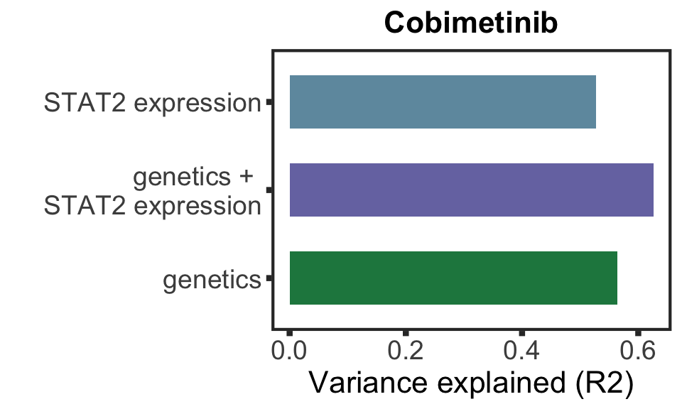
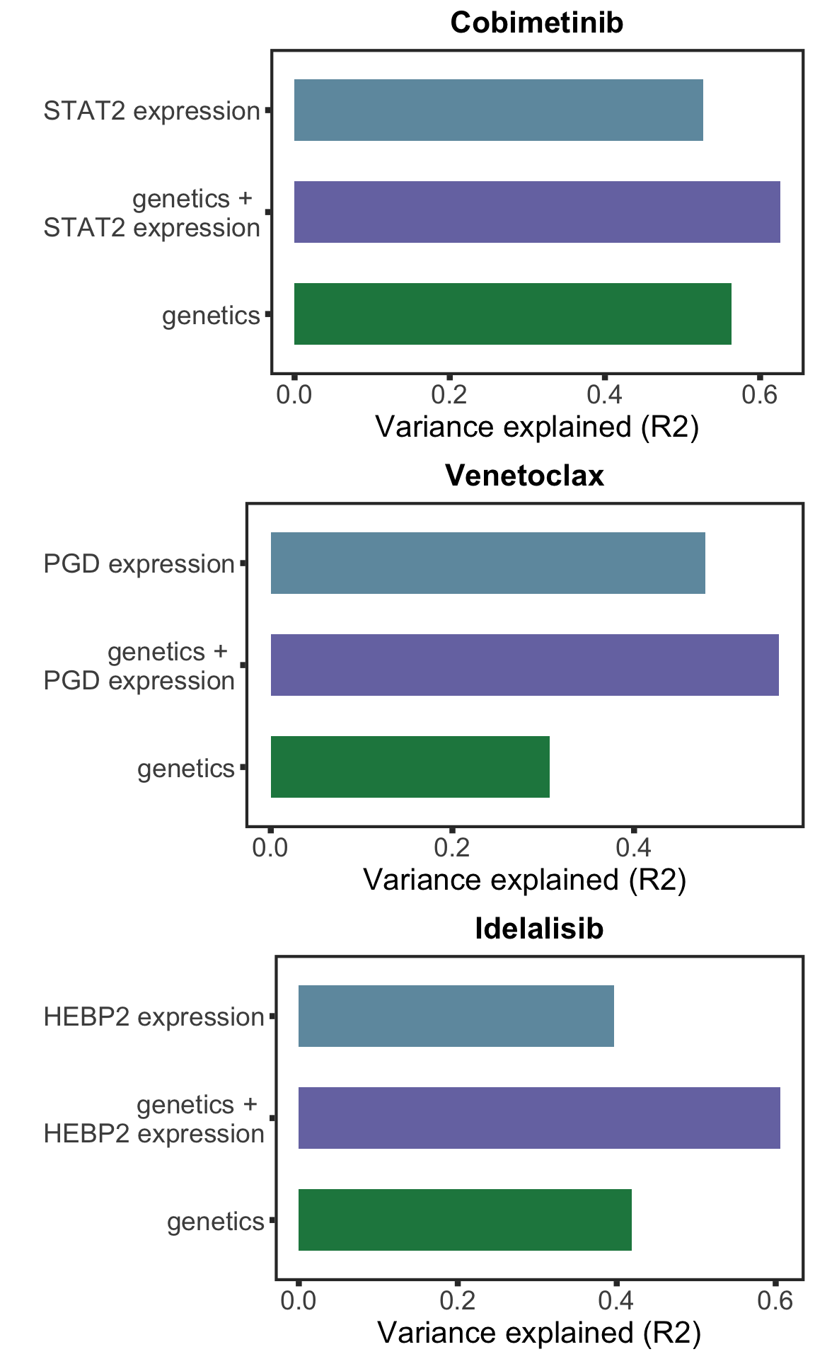
Based on the plot of R2 values, including protein expression in multi-variate model could explain additional variance in drug responses compared to genetic alone. For Venetoclax, using a single protein expression value of PGD already explain more variance than genetics.

stat2Bar <- plotList[[1]]
stat2Bar

Protein markers for clincial outcomes

Uni-variate model to identify proteins associated with outcomes

protCLL.sub <- protCLL[!rowData(protCLL)$chromosome_name %in% c("X","Y"),]
protMat <- assays(protCLL.sub)[["count"]]

survTab <- survT %>% filter(sampleID %in% protCLL$sampleID) %>%
  select(patID,sampleID, OS, died, TTT, treatedAfter) %>%
  dplyr::rename(patientID = patID)
uniRes.ttt <- lapply(rownames(protMat), function(n) {
  testTab <- mutate(survTab, expr = protMat[n, patientID])
  com(testTab$expr, testTab$TTT, testTab$treatedAfter, TRUE) %>%
    mutate(id = n)
}) %>% bind_rows() %>% mutate(p.adj = p.adjust(p, method = "BH")) %>%
  arrange(p) %>% mutate(name = rowData(protCLL[id,])$hgnc_symbol) %>%
  mutate(outcome = "TTT")

uniRes.os <- lapply(rownames(protMat), function(n) {
  testTab <- mutate(survTab, expr = protMat[n, patientID])
  com(testTab$expr, testTab$OS, testTab$died, TRUE) %>%
    mutate(id = n)
}) %>% bind_rows() %>% mutate(p.adj = p.adjust(p, method = "BH")) %>%
  arrange(p) %>% mutate(name = rowData(protCLL[id,])$hgnc_symbol) %>%
  mutate(outcome = "OS")

uniRes <- bind_rows(uniRes.ttt, uniRes.os) %>%
  mutate(p.adj = p.adjust(p, method = "BH"))

A table showing significant associations

uniRes %>% filter(p.adj < 0.1) %>% mutate_if(is.numeric, formatC, digits=2,format="e") %>%
  select(name, p, HR, p.adj, outcome) %>% DT::datatable()

Selection protein markers independent of known risks using multi-vairate model

Prepare data

#table of known risks
riskTab <- select(survTab, patientID, sampleID) %>%
  left_join(patMeta[,c("Patient.ID","IGHV.status","TP53","trisomy12","del17p","gender")], by = c(patientID = "Patient.ID")) %>% 
  mutate(TP53 = as.numeric(as.character(TP53)),
         del17p = as.numeric(as.character(del17p))) %>%
  mutate(`TP53.del17p` = as.numeric(TP53 | del17p),
         IGHV = factor(ifelse(IGHV.status %in% "U",1,0))) %>%
  select(-TP53, -del17p,-IGHV.status) %>%
  mutate_if(is.numeric, as.factor) %>%
  mutate(age = ageTab[match(sampleID, ageTab$sampleID),]$age) %>%
  dplyr::rename(sex=gender) %>%
  mutate(age = age/10) %>% select(-sampleID)

Multi-variate test

cTab.ttt <- lapply(filter(uniRes, outcome == "TTT", p.adj <=0.1)$id, function(n) {
  risk0 <- riskTab
  expr <- protMat[n,]
  expr <- (expr - mean(expr,na.rm=TRUE))/sd(expr,na.rm = TRUE)
  risk1 <- riskTab %>% mutate(protExpr = expr[patientID])
  res0 <- summary(runCox(survTab, risk0, "TTT","treatedAfter"))
  fullModel <- runCox(survTab, risk1, "TTT","treatedAfter")
  res1 <- summary(fullModel)
  tibble(id = n, c0 = res0$concordance[1], c1 = res1$concordance[1],
         se0 = res0$concordance[2],se1 = res1$concordance[2],
         ci0 = se0*1.96, ci1 = se1*1.96,
         p = res1$coefficients["protExpr",5],
         fullModel = list(fullModel))
}) %>% bind_rows() %>% mutate(diffC = c1-c0) %>%
  arrange(desc(diffC)) %>%
  mutate(name=rowData(protCLL[id,])$hgnc_symbol,
         outcome = "TTT")

cTab.os <- lapply(filter(uniRes, outcome == "OS", p.adj<=0.1)$id, function(n) {
  risk0 <- riskTab
  expr <- protMat[n,]
  expr <- (expr - mean(expr,na.rm=TRUE))/sd(expr,na.rm = TRUE)
  risk1 <- riskTab %>% mutate(protExpr = expr[patientID])
  res0 <- summary(runCox(survTab, risk0, "OS","died"))
  fullModel <- runCox(survTab, risk1, "OS","died")
  res1 <- summary(fullModel)
  
  tibble(id = n, c0 = res0$concordance[1], c1 = res1$concordance[1],
         se0 = res0$concordance[2],se1 = res1$concordance[2],
         ci0 = se0*1.96, ci1 = se1*1.96,
         p = res1$coefficients["protExpr",5],
         fullModel = list(fullModel))
}) %>% bind_rows() %>% mutate(diffC = c1-c0) %>%
  arrange(desc(diffC)) %>%
  mutate(name=rowData(protCLL[id,])$hgnc_symbol,
         outcome = "OS")

cTab <- bind_rows(cTab.ttt, cTab.os) %>%
  mutate(p.adj = p.adjust(p, method = "BH")) %>%
  arrange(p)

A table showing idependent protein markers

(We can include this as a supplementary table)

cTab %>% filter(p.adj < 0.1) %>% mutate_if(is.numeric, formatC, digits=2,format="e") %>%
  select(name, p, p.adj, outcome) %>% DT::datatable()

Forest plot of selected markers

plotHazard <- function(survRes, protName, title = "") {
  sumTab <- summary(survRes)$coefficients
  confTab <- summary(survRes)$conf.int
  #correct feature name
  nameOri <- rownames(sumTab)
  nameMod <- substr(nameOri, 1, nchar(nameOri) -1)
  plotTab <- tibble(feature = rownames(sumTab),
                    nameMod = substr(nameOri, 1, nchar(nameOri) -1),
                    HR = sumTab[,2],
                    p = sumTab[,5],
                    Upper = confTab[,4],
                    Lower = confTab[,3]) %>%
    mutate(feature = ifelse(nameMod %in% names(survRes$xlevels), nameMod, feature)) %>%
    mutate(feature = str_replace(feature, "[.]","/")) %>%
    mutate(feature = str_replace(feature, "[_]","-")) %>%
    mutate(candidate = ifelse(feature == "protExpr", "yes","no")) %>%
    mutate(feature = ifelse(feature == "protExpr", protName, feature)) %>%
    arrange(desc(abs(p))) %>% mutate(feature = factor(feature, levels = feature)) #%>%
    #mutate(type = ifelse(HR >1 ,"up","down")) %>%
   # mutate(Upper = ifelse(Upper > 10, 10, Upper))

  p <- ggplot(plotTab, aes(x=feature, y = HR, color = candidate)) +
    geom_hline(yintercept = 1, linetype = "dotted") +
    geom_point(position = position_dodge(width=0.8), size=3) +
    geom_errorbar(aes(ymin = Lower, ymax = Upper), width = 0.3, size=1) +
    geom_text(position = position_nudge(x = 0.3),
              aes(y = HR, label =  sprintf("italic(P)~'='~'%s'",
                                           formatNum(p, digits = 1))),
              color = "black", size =5, parse = TRUE) +
    #expand_limits(y=c(-0.5,0))+
    scale_color_manual(values = c(yes = "darkred", no = "black")) +
    ggtitle(title) + scale_y_log10() +
    ylab("Hazard ratio") +
    coord_flip() +
    theme_full +
    theme(legend.position = "none", axis.title.y = element_blank())
  return(p)
}

PRMT5

protName <- "PRMT5"
outcomeName <- "TTT"
survRes <- filter(cTab, outcome == outcomeName , name == protName)$fullModel[[1]]
hr.prmt5 <- plotHazard(survRes, protName, "Time to treatment")
hr.prmt5

PYGB

protName <- "PYGB"
outcomeName <- "TTT"
survRes <- filter(cTab, outcome == outcomeName , name == protName)$fullModel[[1]]
hr.pygb <- plotHazard(survRes, protName, "Time to treatment")
hr.pygb

PES1

protName <- "PES1"
outcomeName <- "TTT"
survRes <- filter(cTab, outcome == outcomeName , name == protName)$fullModel[[1]]
hr.pes1 <- plotHazard(survRes, protName, "Time to treatment")
hr.pes1

GNAI2

protName <- "GNAI2"
outcomeName <- "OS"
survRes <- filter(cTab, outcome == outcomeName , name == protName)$fullModel[[1]]
plotHazard(survRes, protName, "Overall survival")

RRAS2

protName <- "RRAS2"
outcomeName <- "OS"
survRes <- filter(cTab, outcome == outcomeName , name == protName)$fullModel[[1]]
plotHazard(survRes, protName, "Overall survival")

Bar plots comparing C-index

(Maybe be not necessary in manuscript, I think the forest plots above are better)

TTT

nameList <- c("PRMT5","PYGB","PES1")
cTab.sub <- filter(cTab, outcome == "TTT", name %in% nameList)
plotList <- lapply(seq(nrow(cTab.sub)), function(i) {
  plotTab <- tibble(model = c("knownRisks","plusProtein"),
                    cindex = c(cTab.sub[i,]$c0, cTab.sub[i,]$c1),
                    ci = c(cTab.sub[i,]$ci0,cTab.sub[i,]$ci1))
  ggplot(plotTab, aes(x=model, y=cindex, fill = model)) + 
    geom_bar(stat="identity",width=0.6) + 
    geom_errorbar(aes(ymin=cindex + ci, ymax = cindex-ci), width=0.5) +
    theme_full+ scale_fill_manual(values = colList[6:7]) +
    ggtitle(cTab.ttt[i,]$name) + theme(legend.position = "none") +
    
    ylab("Harrell's C-index")
})
cTTT <- plot_grid(plotlist = plotList, ncol =3)
cTTT

OS (The associations with OS are not very reliable as we don't have enough events)

nameList <- c("GNAI2","RRAS2")
cTab.sub <- filter(cTab, outcome == "OS", name %in% nameList)
plotList <- lapply(seq(nrow(cTab.sub)), function(i) {
  plotTab <- tibble(model = c("knownRisks","plusProtein"),
                    cindex = c(cTab.sub[i,]$c0, cTab.sub[i,]$c1),
                    ci = c(cTab.sub[i,]$ci0,cTab.sub[i,]$ci1))
  ggplot(plotTab, aes(x=model, y=cindex, fill = model)) + 
    geom_bar(stat="identity",width=0.6) + 
    geom_errorbar(aes(ymin=cindex + ci, ymax = cindex-ci), width=0.5) +
    theme_full+ scale_fill_manual(values = colList[6:7]) +
    ggtitle(cTab.ttt[i,]$name) + theme(legend.position = "none") +
    
    ylab("Harrell's C-index")
})
plot_grid(plotlist = plotList, ncol =3)

Assemble figure

Main text figure

#plot_grid(drugBar, drugCor,
#          plot_grid(stat2Bar, cTTT, ncol=2, rel_widths = c(0.3,0.7), labels = c("C","D"), label_size = 20),
#          ncol=1, rel_heights = c(0.4,0.35,0.25), labels = c("A","B"), label_size = 20)
#ggsave("test.pdf", width = 15, height = 15
topFig <- plot_grid(hr.prmt5, hr.pygb, hr.pes1, ncol=3)
midFig <- plot_grid(drugBar, plot_grid(stat2Bar,NULL, rel_heights = c(0.8,0.2), ncol=1), 
                    rel_widths = c(0.6,0.3), labels = c("B","D"), label_size = 20)
botomFig <- drugCor
plot_grid(topFig, NULL, midFig, botomFig, rel_heights = c(0.3,0.02,0.34,0.34),ncol=1,
          labels = c("A","","","C"), label_size = 20)

#ggsave("test.pdf", width = 15, height = 17)

sessionInfo()
R version 3.6.0 (2019-04-26)
Platform: x86_64-apple-darwin15.6.0 (64-bit)
Running under: macOS  10.15.6

Matrix products: default
BLAS:   /Library/Frameworks/R.framework/Versions/3.6/Resources/lib/libRblas.0.dylib
LAPACK: /Library/Frameworks/R.framework/Versions/3.6/Resources/lib/libRlapack.dylib

locale:
[1] en_US.UTF-8/en_US.UTF-8/en_US.UTF-8/C/en_US.UTF-8/en_US.UTF-8

attached base packages:
[1] parallel  stats4    stats     graphics  grDevices utils     datasets 
[8] methods   base     

other attached packages:
 [1] latex2exp_0.4.0             forcats_0.5.0              
 [3] stringr_1.4.0               dplyr_1.0.0                
 [5] purrr_0.3.4                 readr_1.3.1                
 [7] tidyr_1.1.0                 tibble_3.0.3               
 [9] tidyverse_1.3.0             cowplot_1.0.0              
[11] SummarizedExperiment_1.16.1 DelayedArray_0.12.3        
[13] BiocParallel_1.20.1         matrixStats_0.56.0         
[15] Biobase_2.46.0              GenomicRanges_1.38.0       
[17] GenomeInfoDb_1.22.1         IRanges_2.20.2             
[19] S4Vectors_0.24.4            BiocGenerics_0.32.0        
[21] glmnet_4.0-2                Matrix_1.2-18              
[23] maxstat_0.7-25              survminer_0.4.7            
[25] ggpubr_0.4.0                ggplot2_3.3.2              
[27] survival_3.2-3              jyluMisc_0.1.5             
[29] pheatmap_1.0.12             limma_3.42.2               

loaded via a namespace (and not attached):
  [1] readxl_1.3.1           backports_1.1.8        fastmatch_1.1-0       
  [4] drc_3.0-1              workflowr_1.6.2        igraph_1.2.5          
  [7] shinydashboard_0.7.1   splines_3.6.0          crosstalk_1.1.0.1     
 [10] TH.data_1.0-10         digest_0.6.25          foreach_1.5.0         
 [13] htmltools_0.5.0        fansi_0.4.1            gdata_2.18.0          
 [16] memoise_1.1.0          magrittr_1.5           cluster_2.1.0         
 [19] openxlsx_4.1.5         annotate_1.64.0        modelr_0.1.8          
 [22] sandwich_2.5-1         piano_2.2.0            colorspace_1.4-1      
 [25] rvest_0.3.5            blob_1.2.1             haven_2.3.1           
 [28] xfun_0.15              crayon_1.3.4           RCurl_1.98-1.2        
 [31] jsonlite_1.7.0         genefilter_1.68.0      zoo_1.8-8             
 [34] iterators_1.0.12       glue_1.4.1             gtable_0.3.0          
 [37] zlibbioc_1.32.0        XVector_0.26.0         car_3.0-8             
 [40] shape_1.4.4            abind_1.4-5            scales_1.1.1          
 [43] mvtnorm_1.1-1          DBI_1.1.0              relations_0.6-9       
 [46] rstatix_0.6.0          Rcpp_1.0.5             plotrix_3.7-8         
 [49] xtable_1.8-4           bit_4.0.4              foreign_0.8-71        
 [52] km.ci_0.5-2            DT_0.14                htmlwidgets_1.5.1     
 [55] httr_1.4.1             fgsea_1.12.0           gplots_3.0.4          
 [58] RColorBrewer_1.1-2     ellipsis_0.3.1         farver_2.0.3          
 [61] XML_3.98-1.20          pkgconfig_2.0.3        dbplyr_1.4.4          
 [64] labeling_0.3           AnnotationDbi_1.48.0   tidyselect_1.1.0      
 [67] rlang_0.4.7            later_1.1.0.1          munsell_0.5.0         
 [70] cellranger_1.1.0       tools_3.6.0            visNetwork_2.0.9      
 [73] cli_2.0.2              RSQLite_2.2.0          generics_0.0.2        
 [76] broom_0.7.0            evaluate_0.14          fastmap_1.0.1         
 [79] yaml_2.2.1             bit64_0.9-7            knitr_1.29            
 [82] fs_1.4.2               zip_2.0.4              survMisc_0.5.5        
 [85] caTools_1.18.0         nlme_3.1-148           mime_0.9              
 [88] slam_0.1-47            xml2_1.3.2             compiler_3.6.0        
 [91] rstudioapi_0.11        curl_4.3               ggsignif_0.6.0        
 [94] marray_1.64.0          reprex_0.3.0           stringi_1.4.6         
 [97] lattice_0.20-41        shinyjs_1.1            KMsurv_0.1-5          
[100] vctrs_0.3.1            pillar_1.4.6           lifecycle_0.2.0       
[103] data.table_1.12.8      bitops_1.0-6           httpuv_1.5.4          
[106] R6_2.4.1               promises_1.1.1         KernSmooth_2.23-17    
[109] gridExtra_2.3          rio_0.5.16             codetools_0.2-16      
[112] MASS_7.3-51.6          gtools_3.8.2           exactRankTests_0.8-31 
[115] assertthat_0.2.1       rprojroot_1.3-2        withr_2.2.0           
[118] multcomp_1.4-13        GenomeInfoDbData_1.2.2 mgcv_1.8-31           
[121] hms_0.5.3              grid_3.6.0             rmarkdown_2.3         
[124] carData_3.0-4          git2r_0.27.1           sets_1.0-18           
[127] lubridate_1.7.9        shiny_1.5.0