Association with clincial outcome based on proteomics data
Junyan Lu
2020-03-10
Last updated: 2020-06-06
Checks: 6 1
Knit directory: Proteomics/analysis/
This reproducible R Markdown analysis was created with workflowr (version 1.6.0). The Checks tab describes the reproducibility checks that were applied when the results were created. The Past versions tab lists the development history.
The R Markdown file has unstaged changes. To know which version of the R Markdown file created these results, you’ll want to first commit it to the Git repo. If you’re still working on the analysis, you can ignore this warning. When you’re finished, you can run wflow_publish to commit the R Markdown file and build the HTML.
Great job! The global environment was empty. Objects defined in the global environment can affect the analysis in your R Markdown file in unknown ways. For reproduciblity it’s best to always run the code in an empty environment.
The command set.seed(20200227) was run prior to running the code in the R Markdown file. Setting a seed ensures that any results that rely on randomness, e.g. subsampling or permutations, are reproducible.
Great job! Recording the operating system, R version, and package versions is critical for reproducibility.
Nice! There were no cached chunks for this analysis, so you can be confident that you successfully produced the results during this run.
Great job! Using relative paths to the files within your workflowr project makes it easier to run your code on other machines.
Great! You are using Git for version control. Tracking code development and connecting the code version to the results is critical for reproducibility. The version displayed above was the version of the Git repository at the time these results were generated.
Note that you need to be careful to ensure that all relevant files for the analysis have been committed to Git prior to generating the results (you can use wflow_publish or wflow_git_commit). workflowr only checks the R Markdown file, but you know if there are other scripts or data files that it depends on. Below is the status of the Git repository when the results were generated:
Ignored files:
    Ignored:    .DS_Store
    Ignored:    .Rhistory
    Ignored:    .Rproj.user/
    Ignored:    analysis/.DS_Store
    Ignored:    analysis/.Rhistory
    Ignored:    analysis/complexAnalysis_IGHV_alternative_cache/
    Ignored:    analysis/complexAnalysis_IGHV_cache/
    Ignored:    analysis/complexAnalysis_trisomy12_alteredPQR_cache/
    Ignored:    analysis/complexAnalysis_trisomy12_alternative_cache/
    Ignored:    analysis/complexAnalysis_trisomy12_cache/
    Ignored:    analysis/correlateCLLPD_cache/
    Ignored:    code/.Rhistory
    Ignored:    data/.DS_Store
    Ignored:    output/.DS_Store

Untracked files:
    Untracked:  analysis/CNVanalysis_11q.Rmd
    Untracked:  analysis/CNVanalysis_trisomy12.Rmd
    Untracked:  analysis/CNVanalysis_trisomy19.Rmd
    Untracked:  analysis/analysisPCA.Rmd
    Untracked:  analysis/analysisSplicing.Rmd
    Untracked:  analysis/analysisTrisomy19.Rmd
    Untracked:  analysis/annotateCNV.Rmd
    Untracked:  analysis/complexAnalysis_IGHV.Rmd
    Untracked:  analysis/complexAnalysis_IGHV_alternative.Rmd
    Untracked:  analysis/complexAnalysis_overall.Rmd
    Untracked:  analysis/complexAnalysis_trisomy12.Rmd
    Untracked:  analysis/complexAnalysis_trisomy12_alternative.Rmd
    Untracked:  analysis/correlateGenomic_PC12adjusted.Rmd
    Untracked:  analysis/correlateGenomic_noBlock.Rmd
    Untracked:  analysis/correlateGenomic_noBlock_MCLL.Rmd
    Untracked:  analysis/correlateGenomic_noBlock_UCLL.Rmd
    Untracked:  analysis/default.css
    Untracked:  analysis/del11q.pdf
    Untracked:  analysis/del11q_norm.pdf
    Untracked:  analysis/peptideValidate.Rmd
    Untracked:  analysis/plotExpressionCNV.Rmd
    Untracked:  analysis/processPeptides_LUMOS.Rmd
    Untracked:  analysis/style.css
    Untracked:  analysis/trisomy12.pdf
    Untracked:  analysis/trisomy12_AFcor.Rmd
    Untracked:  analysis/trisomy12_norm.pdf
    Untracked:  code/AlteredPQR.R
    Untracked:  code/utils.R
    Untracked:  data/190909_CLL_prot_abund_med_norm.tsv
    Untracked:  data/190909_CLL_prot_abund_no_norm.tsv
    Untracked:  data/20190423_Proteom_submitted_samples_bereinigt.xlsx
    Untracked:  data/20191025_Proteom_submitted_samples_final.xlsx
    Untracked:  data/LUMOS/
    Untracked:  data/LUMOS_peptides/
    Untracked:  data/LUMOS_protAnnotation.csv
    Untracked:  data/LUMOS_protAnnotation_fix.csv
    Untracked:  data/SampleAnnotation_cleaned.xlsx
    Untracked:  data/example_proteomics_data
    Untracked:  data/facTab_IC50atLeast3New.RData
    Untracked:  data/gmts/
    Untracked:  data/mapEnsemble.txt
    Untracked:  data/mapSymbol.txt
    Untracked:  data/proteins_in_complexes
    Untracked:  data/pyprophet_export_aligned.csv
    Untracked:  data/timsTOF_protAnnotation.csv
    Untracked:  output/LUMOS_processed.RData
    Untracked:  output/cnv_plots.zip
    Untracked:  output/cnv_plots/
    Untracked:  output/cnv_plots_norm.zip
    Untracked:  output/dxdCLL.RData
    Untracked:  output/exprCNV.RData
    Untracked:  output/pepCLL_lumos.RData
    Untracked:  output/pepTab_lumos.RData
    Untracked:  output/plotCNV_allChr11_diff.pdf
    Untracked:  output/plotCNV_del11q_sum.pdf
    Untracked:  output/proteomic_LUMOS_20200227.RData
    Untracked:  output/proteomic_LUMOS_20200320.RData
    Untracked:  output/proteomic_LUMOS_20200430.RData
    Untracked:  output/proteomic_timsTOF_20200227.RData
    Untracked:  output/splicingResults.RData
    Untracked:  output/timsTOF_processed.RData
    Untracked:  plotCNV_del11q_diff.pdf

Unstaged changes:
    Modified:   analysis/_site.yml
    Modified:   analysis/analysisSF3B1.Rmd
    Modified:   analysis/compareProteomicsRNAseq.Rmd
    Modified:   analysis/correlateCLLPD.Rmd
    Modified:   analysis/correlateGenomic.Rmd
    Deleted:    analysis/correlateGenomic_removePC.Rmd
    Modified:   analysis/correlateMIR.Rmd
    Modified:   analysis/correlateMethylationCluster.Rmd
    Modified:   analysis/index.Rmd
    Modified:   analysis/predictOutcome.Rmd
    Modified:   analysis/processProteomics_LUMOS.Rmd
    Modified:   analysis/qualityControl_LUMOS.Rmd
Note that any generated files, e.g. HTML, png, CSS, etc., are not included in this status report because it is ok for generated content to have uncommitted changes.
These are the previous versions of the R Markdown and HTML files. If you’ve configured a remote Git repository (see ?wflow_git_remote), click on the hyperlinks in the table below to view them.
| File | Version | Author | Date | Message |
|---|---|---|---|---|
| html | b8e0823 | Junyan Lu | 2020-03-10 | Build site. |
| Rmd | c8cb45c | Junyan Lu | 2020-03-10 | update analysis |
Association between PCs and clinical outcomes
PCA
Get top 1000 most variant genes
#remove genes on sex chromosomes
protCLL.sub <- protCLL[!rowData(protCLL)$chromosome_name %in% c("X","Y"),]
plotMat <- assays(protCLL.sub)[["QRILC"]]

sds <- genefilter::rowSds(plotMat)
plotMat <- as.matrix(plotMat[order(sds,decreasing = TRUE)[1:1000],])

colAnno <- colData(protCLL)[,c("gender","IGHV.status","trisomy12")] %>%
  data.frame()
PCA
pcRes <- prcomp(t(plotMat), center =TRUE, scale. = TRUE)
pcTab <- pcRes$x
plotTab <- pcTab[,1:4] %>% data.frame() %>% cbind(colAnno[rownames(.),]) %>%
  rownames_to_column("patID") %>% as_tibble()

ggplot(plotTab, aes(x=PC1, y=PC2, shape = IGHV.status, col = trisomy12)) + geom_point() 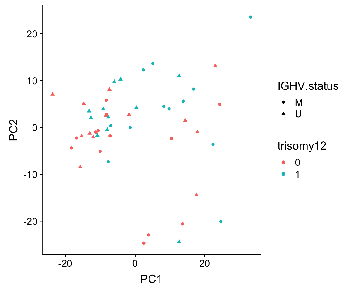
| Version | Author | Date |
|---|---|---|
| b8e0823 | Junyan Lu | 2020-03-10 |
ggplot(plotTab, aes(x=PC3, y=PC4, shape = IGHV.status, col = trisomy12)) + geom_point() 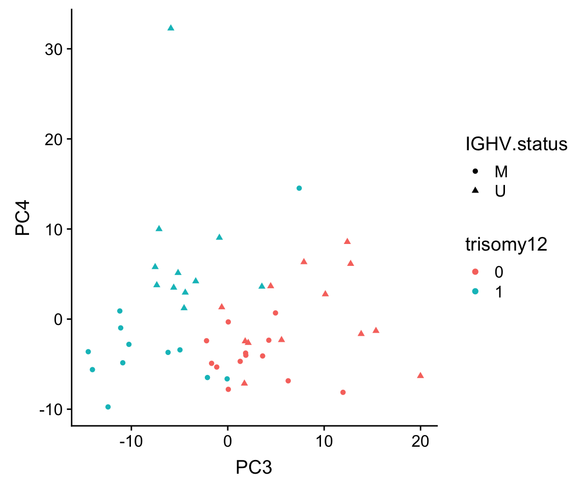
| Version | Author | Date |
|---|---|---|
| b8e0823 | Junyan Lu | 2020-03-10 |
testTab <- pcTab[,1:10] %>% data.frame() %>%
  rownames_to_column("patientID") %>% mutate(sampleID = protCLL[,patientID]$sampleID) %>%
  gather(key = "factor", value = "value", -patientID, -sampleID) %>%
  left_join(survT, by = "sampleID")

#for OS
resOS <- filter(testTab, !is.na(OS)) %>%
  group_by(factor) %>%
  do(com(.$value, .$OS, .$died, TRUE)) %>% ungroup() %>%
  arrange(p) %>% mutate(p.adj = p.adjust(p, method = "BH")) %>%
  mutate(Endpoint = "OS")

#for TTT
resTTT <- filter(testTab, !is.na(TTT)) %>%
  group_by(factor) %>%
  do(com(.$value, .$TTT, .$treatedAfter, TRUE)) %>% ungroup() %>%
  arrange(p) %>% mutate(p.adj = p.adjust(p, method = "BH")) %>%
  mutate(Endpoint = "TTT")
Plot p value and hazard ratio
plotTab <- bind_rows(resOS, resTTT) %>%
 filter(factor %in% c("PC3","PC4","PC5","PC7"))

haPlot <- ggplot(plotTab, aes(x=factor, y = HR, col = Endpoint, dodge = Endpoint)) +
  geom_hline(yintercept = 1, linetype = "dotted") +
  geom_point(position = position_dodge(width=0.8)) +
  geom_errorbar(position = position_dodge(width =0.8),
                aes(ymin = lower, ymax = higher), width = 0.3, size=1) +
  geom_text(position = position_dodge2(width = 0.8),
            aes(x=as.numeric(as.factor(factor))+0.15,
                label = sprintf("italic(P)~'='~'%s'",
                                formatNum(p))),
            color = "black",size =5, parse = TRUE) +
  xlab("Factor") + ylab("Hazard ratio") +
  scale_y_log10(limits = c(0.1,15)) +
  coord_flip() + theme_bw() + theme(legend.title = element_blank(),
                                    legend.position = c(0.2,0.1),
                                    legend.background = element_blank(),
                                    legend.key.size = unit(0.5,"cm"),
                                    legend.key.width = unit(0.6,"cm"),
                                    legend.text = element_text(size=rel(1.2)))

haPlot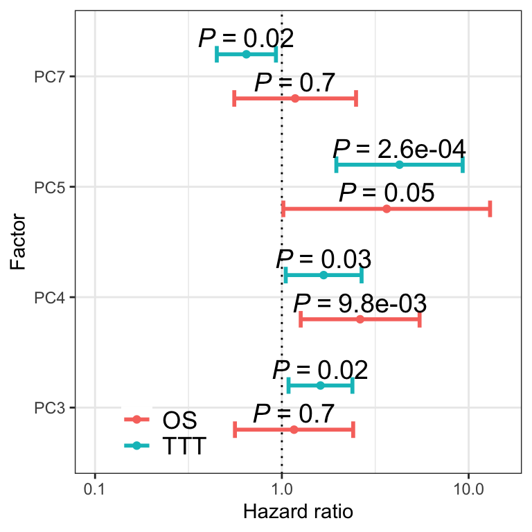
| Version | Author | Date |
|---|---|---|
| b8e0823 | Junyan Lu | 2020-03-10 |
Kaplan-Meiler plots
KM plot for overall survival (OS)
facList <- sort(filter(resOS, p.adj <=0.3)$factor)
osList <- lapply(facList, function(x) {
  eachTab <- filter(testTab, factor == x) %>%
    select(value, OS, died) %>% filter(!is.na(OS))
  pval <- filter(resOS, factor == x)$p
  km(eachTab$value, eachTab$OS, eachTab$died, sprintf("%s VS Overall survival time", x),
     stat = "maxstat", pval = pval, showTable = TRUE)
})
Warning: Vectorized input to `element_text()` is not officially supported.
Results may be unexpected or may change in future versions of ggplot2.Warning in is.na(x): is.na() applied to non-(list or vector) of type
'language'Warning in fitter(X, Y, strats, offset, init, control, weights = weights, :
Loglik converged before variable 1 ; coefficient may be infinite.Warning: Vectorized input to `element_text()` is not officially supported.
Results may be unexpected or may change in future versions of ggplot2.Warning in is.na(x): is.na() applied to non-(list or vector) of type
'language'plot_grid(plotlist = osList)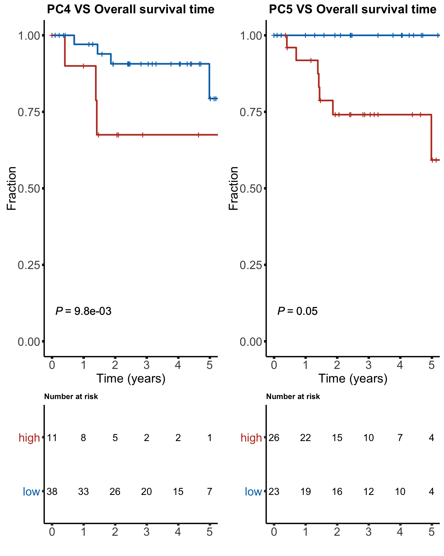
| Version | Author | Date |
|---|---|---|
| b8e0823 | Junyan Lu | 2020-03-10 |
KM plot for time to treatment (TTT)
facList <- sort(filter(resTTT, p.adj <=0.1)$factor)
tttList <- lapply(facList, function(x) {
  eachTab <- filter(testTab, factor == x) %>%
    select(value, TTT, treatedAfter) %>% filter(!is.na(TTT))
    pval <- filter(resTTT, factor == x)$p
  km(eachTab$value, eachTab$TTT, eachTab$treatedAfter, sprintf("%s VS Time to treatment", x), stat = "maxstat",
     maxTime = 7, pval = pval, showTable = TRUE)
})
Warning: Vectorized input to `element_text()` is not officially supported.
Results may be unexpected or may change in future versions of ggplot2.Warning in is.na(x): is.na() applied to non-(list or vector) of type
'language'Warning: Vectorized input to `element_text()` is not officially supported.
Results may be unexpected or may change in future versions of ggplot2.Warning in is.na(x): is.na() applied to non-(list or vector) of type
'language'Warning: Vectorized input to `element_text()` is not officially supported.
Results may be unexpected or may change in future versions of ggplot2.Warning in is.na(x): is.na() applied to non-(list or vector) of type
'language'Warning: Vectorized input to `element_text()` is not officially supported.
Results may be unexpected or may change in future versions of ggplot2.Warning in is.na(x): is.na() applied to non-(list or vector) of type
'language'plot_grid(plotlist = tttList, ncol = 2)
| Version | Author | Date |
|---|---|---|
| b8e0823 | Junyan Lu | 2020-03-10 |
Correlation between PCs and CLL-PD
load("../data/facTab_IC50atLeast3New.RData")
testTab.LF <- mutate(testTab, LF4 = facTab[match(patientID, facTab$patID),]$factor) %>%
  filter(!is.na(LF4)) %>% select(factor, value, LF4)
testRes <- group_by(testTab.LF, factor) %>% nest() %>%
  mutate(m = map(data, ~cor.test(~LF4 + value, .))) %>%
  mutate(res = map(m, broom::tidy)) %>%
  unnest(res) %>%
  select(factor, p.value) %>% dplyr::rename(PC = factor) %>%
  arrange(p.value)
head(testRes)
# A tibble: 6 x 2
# Groups: PC [6]
PC p.value
<chr> <dbl>
1 PC5 0.00102
2 PC4 0.00167
3 PC8 0.151
4 PC2 0.307
5 PC7 0.348
6 PC10 0.360 Both PC4 and PC5 are associated with CLL-PD
Select independent protein markers for outcome prediction
Prepare data
protCLL.sub <- protCLL[!rowData(protCLL)$chromosome_name %in% c("X","Y"),]
protMat <- assays(protCLL.sub)[["QRILC"]]

survTab <- survT %>% filter(sampleID %in% protCLL$sampleID) %>%
  select(patID,sampleID, OS, died, TTT, treatedAfter) %>%
  dplyr::rename(patientID = patID)
Univariate test
uniRes.ttt <- lapply(rownames(protMat), function(n) {
  testTab <- mutate(survTab, expr = protMat[n, patientID])
  com(testTab$expr, testTab$TTT, testTab$treatedAfter, TRUE) %>%
    mutate(id = n)
}) %>% bind_rows() %>% mutate(p.adj = p.adjust(p, method = "BH")) %>%
  arrange(p) %>% mutate(name = rowData(protCLL[id,])$hgnc_symbol)

uniRes.os <- lapply(rownames(protMat), function(n) {
  testTab <- mutate(survTab, expr = protMat[n, patientID])
  com(testTab$expr, testTab$OS, testTab$died, TRUE) %>%
    mutate(id = n)
}) %>% bind_rows() %>% mutate(p.adj = p.adjust(p, method = "BH")) %>%
  arrange(p) %>% mutate(name = rowData(protCLL[id,])$hgnc_symbol)
Table for TTT
uniRes.ttt %>% filter(p < 0.05) %>% mutate_if(is.numeric, formatC, digits=2,format="e") %>%
  select(name, p, HR, p.adj) %>% DT::datatable()
Table for OS
uniRes.os %>% filter(p < 0.05) %>% mutate_if(is.numeric, formatC, digits=2,format="e") %>%
  select(name, p, HR, p.adj) %>% DT::datatable()
P-value histogram
plotTab <- mutate(uniRes.ttt, outcome = "TTT") %>% bind_rows(mutate(uniRes.os, outcome = "OS"))
ggplot(plotTab, aes(x=p, fill = outcome)) + geom_histogram(bins = 50) + facet_wrap(~outcome) +
  theme(legend.position = "none")+ xlim(0,1)
Warning: Removed 4 rows containing missing values (geom_bar).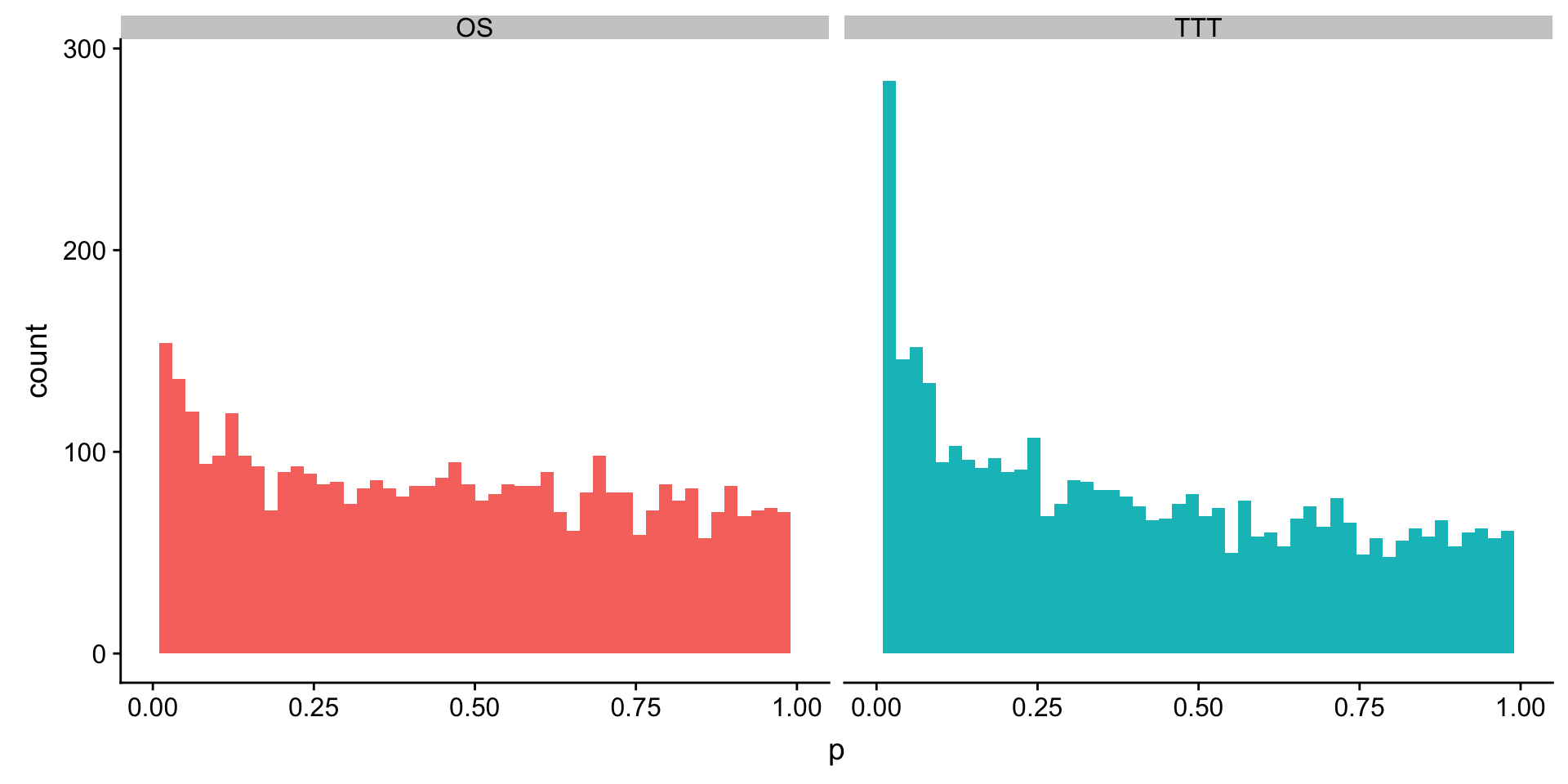
| Version | Author | Date |
|---|---|---|
| b8e0823 | Junyan Lu | 2020-03-10 |
Selection using multi-vairate model
Prepare data
#table of known risks
riskTab <- select(survTab, patientID, sampleID) %>%
  left_join(patMeta[,c("Patient.ID","IGHV.status","TP53","trisomy12","del17p","gender")], by = c(patientID = "Patient.ID")) %>%
  mutate(TP53 = as.numeric(as.character(TP53)),
         del17p = as.numeric(as.character(del17p))) %>%
  mutate(`TP53.del17p` = as.numeric(TP53 | del17p)) %>%
  select(-TP53, -del17p) %>%
  mutate_if(is.numeric, as.factor) %>%
  mutate(age = ageTab[match(sampleID, ageTab$sampleID),]$age) %>%
  dplyr::rename(sex=gender) %>%
  mutate(age = age/10) %>% select(-sampleID)
Select based on C-index
TTT
cTab.ttt <- lapply(filter(uniRes.ttt, p<=0.05)$id, function(n) {
  risk0 <- riskTab
  risk1 <- riskTab %>% mutate(protExpr = protMat[n,patientID])
  res0 <- summary(runCox(survTab, risk0, "TTT","treatedAfter"))
  res1 <- summary(runCox(survTab, risk1, "TTT","treatedAfter"))
  tibble(id = n, c0 = res0$concordance[1], c1 = res1$concordance[1],
         se0 = res0$concordance[2],se1 = res1$concordance[2],
         ci0 = se0*1.96, ci1 = se1*1.96)
}) %>% bind_rows() %>% mutate(diffC = c1-c0) %>%
  arrange(desc(diffC)) %>%
  mutate(name=rowData(protCLL[id,])$hgnc_symbol)
Plot top 9 candidates
plotList <- lapply(1:9, function(i) {
  plotTab <- tibble(model = c("knownRisks","plusProtein"),
                    cindex = c(cTab.ttt[i,]$c0, cTab.ttt[i,]$c1),
                    ci = c(cTab.ttt[i,]$ci0,cTab.ttt[i,]$ci1))
  ggplot(plotTab, aes(x=model, y=cindex, fill = model)) +
    geom_bar(stat="identity",width=0.8) +
    geom_errorbar(aes(ymin=cindex + ci, ymax = cindex-ci), width=0.5) +
    ggtitle(cTab.ttt[i,]$name) + theme(legend.position = "none") +
    ylab("Harrell's C-index")
})
plot_grid(plotlist = plotList, ncol =3)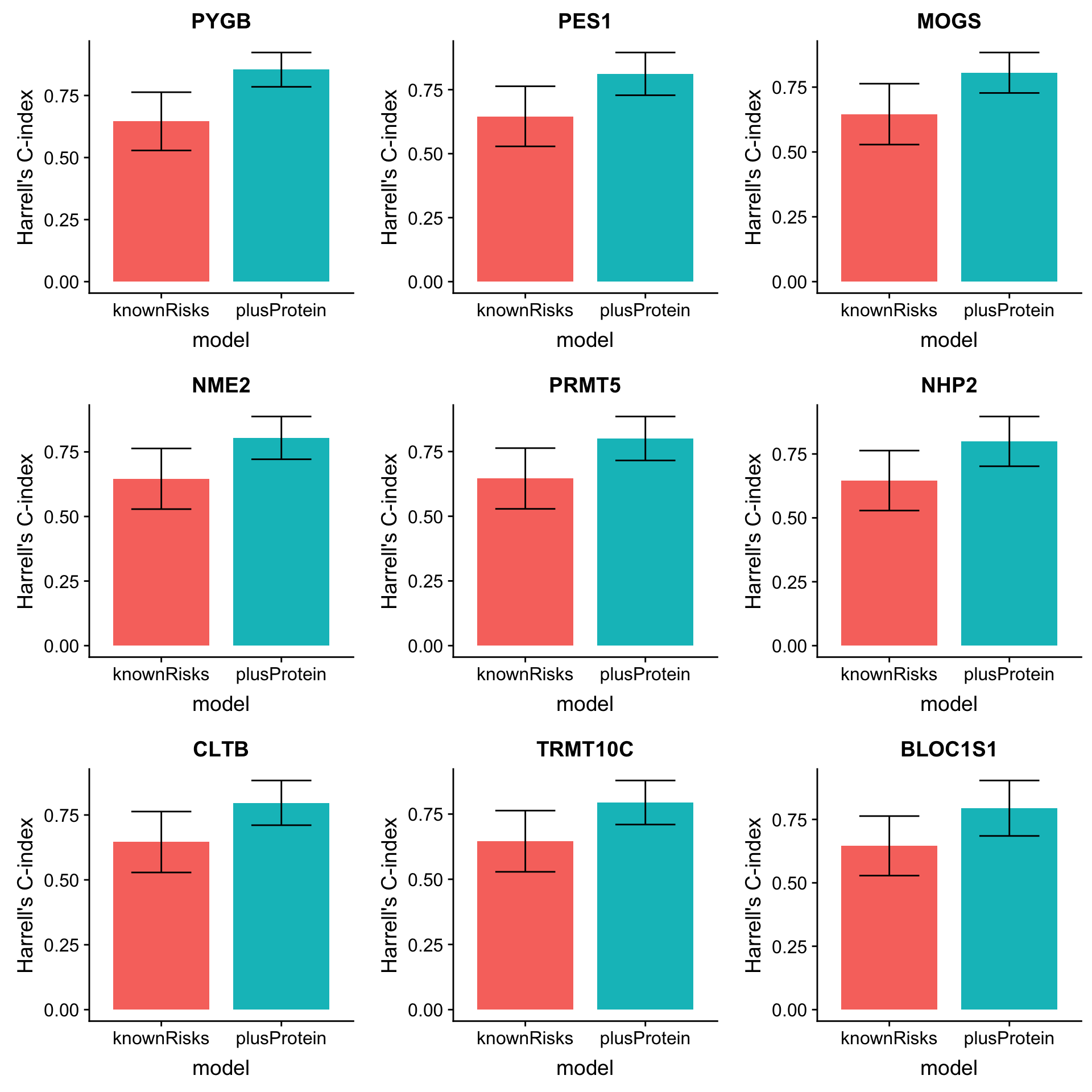
| Version | Author | Date |
|---|---|---|
| b8e0823 | Junyan Lu | 2020-03-10 |
OS
cTab.os <- lapply(filter(uniRes.os, p<=0.05)$id, function(n) {
  risk0 <- riskTab
  risk1 <- riskTab %>% mutate(protExpr = protMat[n,patientID])
  res0 <- summary(runCox(survTab, risk0, "OS","died"))
  res1 <- tryCatch({
    summary(runCox(survTab, risk1, "OS","died"))
  }, error = function(err) {
    list(concordance = c(NA,NA))
  })

  tibble(id = n, c0 = res0$concordance[1], c1 = res1$concordance[1],
         se0 = res0$concordance[2],se1 = res1$concordance[2],
         ci0 = se0*1.96, ci1 = se1*1.96)
}) %>% bind_rows() %>% mutate(diffC = c1-c0) %>%
  arrange(desc(diffC)) %>%
  mutate(name=rowData(protCLL[id,])$hgnc_symbol)
Plot top 9 candidates
plotList <- lapply(1:9, function(i) {
  plotTab <- tibble(model = c("knownRisks","plusProtein"),
                    cindex = c(cTab.os[i,]$c0, cTab.os[i,]$c1),
                    ci = c(cTab.os[i,]$ci0,cTab.os[i,]$ci1))
  ggplot(plotTab, aes(x=model, y=cindex, fill = model)) +
    geom_bar(stat="identity",width=0.8) +
    geom_errorbar(aes(ymin=cindex + ci, ymax = cindex-ci), width=0.5) +
    ggtitle(cTab.os[i,]$name) + theme(legend.position = "none") +
    ylab("Harrell's C-index")
})
plot_grid(plotlist = plotList, ncol =3)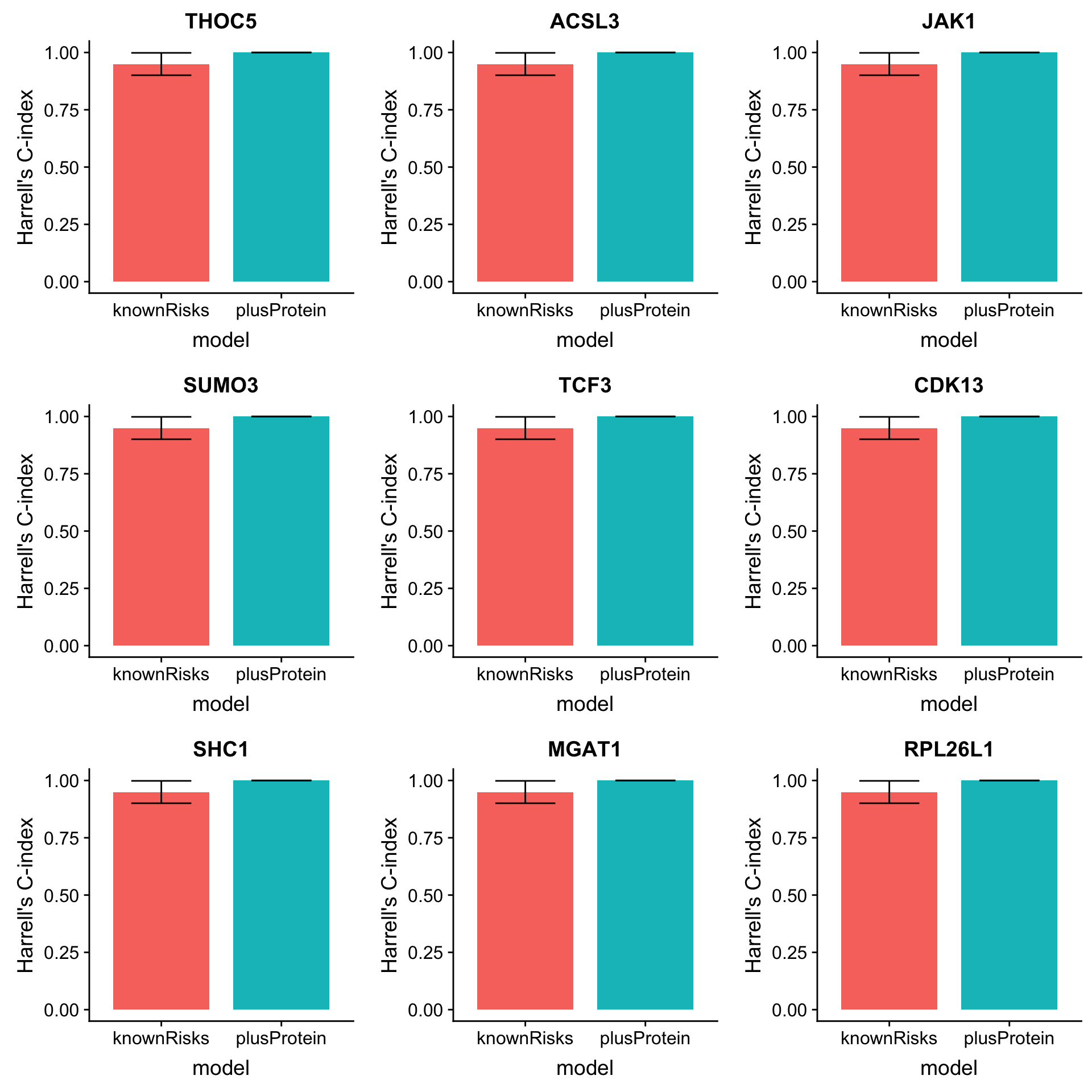
| Version | Author | Date |
|---|---|---|
| b8e0823 | Junyan Lu | 2020-03-10 |
Compare the ability of RNAseq data and proteomic data for predicting outcome
Data processing
Prepare survival table
#table of known risks
survTab <- survT %>%
  select(patID,sampleID, OS, died, TTT, treatedAfter) %>%
  dplyr::rename(patientID = patID) %>%
  filter(!(is.na(OS) &is.na(TTT)))
Processing RNAseq data
load("../../var/ddsrna_180717.RData")
ddsSub <- dds[,dds$diag %in% "CLL" & dds$PatID %in% survTab$patientID]
#ddsSub <- ddsSub[rowData(ddsSub)$symbol %in% rowData(protCLL)$hgnc_symbol,]
ddsSub <- ddsSub[!rowData(ddsSub)$symbol %in% c(NA,"")]
ddsSub <- ddsSub[rowData(ddsSub)$biotype %in% "protein_coding"]
ddsSub <- ddsSub[!rowData(ddsSub)$chromosome %in% c("X","Y"),]
ddsSub <- ddsSub[rowSums(counts(ddsSub, normalized = TRUE)) > 100, ]
ddsSub.vst <- varianceStabilizingTransformation(ddsSub)
sds <- genefilter::rowSds(assay(ddsSub.vst))
ddsSub.vst <- ddsSub.vst[sds > genefilter::shorth(sds),]
rnaMat <- assay(ddsSub.vst)
rownames(rnaMat) <- rowData(ddsSub.vst)$symbol
Outcome prediction with RNAseq data
Full RNAseq dataset
Univariate test
survTab.rna <- filter(survTab, sampleID %in% ddsSub.vst$sampleID)
rnaUniRes <- list()
rnaUniRes[["full"]] <- list()

rnaUniRes[["full"]][["TTT"]] <- lapply(rownames(rnaMat), function(n) {
  testTab <- mutate(survTab.rna, expr = rnaMat[n, patientID])
  com(testTab$expr, testTab$TTT, testTab$treatedAfter, TRUE) %>%
    mutate(name = n)
}) %>% bind_rows() %>% mutate(p.adj = p.adjust(p, method = "BH")) %>%
  arrange(p)

rnaUniRes[["full"]][["OS"]] <- lapply(rownames(rnaMat), function(n) {
  testTab <- mutate(survTab.rna, expr = rnaMat[n, patientID])
  com(testTab$expr, testTab$OS, testTab$died, TRUE) %>%
    mutate(name = n)
}) %>% bind_rows() %>% mutate(p.adj = p.adjust(p, method = "BH")) %>%
  arrange(p)
P-value histogram
plotTab <- mutate(rnaUniRes$full$TTT, outcome = "TTT") %>% bind_rows(mutate(rnaUniRes$full$OS, outcome = "OS"))
ggplot(plotTab, aes(x=p, fill = outcome)) + geom_histogram(bins = 50) + facet_wrap(~outcome, scale = "free") +
  theme(legend.position = "none")+ xlim(0,1)
Warning: Removed 4 rows containing missing values (geom_bar).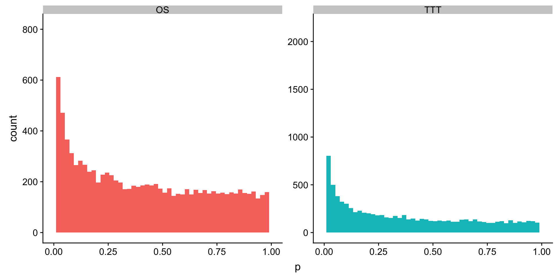
| Version | Author | Date |
|---|---|---|
| b8e0823 | Junyan Lu | 2020-03-10 |
Multi-variate model
Prepare table for known genomic risks
riskTab.rna <- select(survTab.rna, patientID, sampleID) %>%
  left_join(patMeta[,c("Patient.ID","IGHV.status","TP53","trisomy12","del17p","gender")], by = c(patientID = "Patient.ID")) %>%
  mutate(TP53 = as.numeric(as.character(TP53)),
         del17p = as.numeric(as.character(del17p))) %>%
  mutate(`TP53.del17p` = as.numeric(TP53 | del17p)) %>%
  select(-TP53, -del17p) %>%
  mutate_if(is.numeric, as.factor) %>%
  mutate(age = ageTab[match(sampleID, ageTab$sampleID),]$age) %>%
  dplyr::rename(sex=gender) %>%
  mutate(age = age/10) %>% select(-sampleID)
TTT
rnaMultiRes <- list()
rnaMultiRes[["full"]] <- list()

rnaMultiRes[["full"]][["TTT"]] <- lapply(filter(rnaUniRes[["full"]][["TTT"]], p<=0.05)$name, function(n) {
  risk0 <- riskTab.rna
  risk1 <- riskTab.rna %>% mutate(protExpr = rnaMat[n,patientID])
  res0 <- summary(runCox(survTab.rna, risk0, "TTT","treatedAfter"))
  res1 <- summary(runCox(survTab.rna, risk1, "TTT","treatedAfter"))
  tibble(name = n, c0 = res0$concordance[1], c1 = res1$concordance[1],
         se0 = res0$concordance[2],se1 = res1$concordance[2],
         ci0 = se0*1.96, ci1 = se1*1.96)
}) %>% bind_rows() %>% mutate(diffC = c1-c0) %>%
  arrange(desc(diffC))
Plot top 9 candidates
plotList <- lapply(1:9, function(i) {
  plotTab <- tibble(model = c("knownRisks","plusRNA"),
                    cindex = c(rnaMultiRes[["full"]][["TTT"]][i,]$c0, rnaMultiRes[["full"]][["TTT"]][i,]$c1),
                    ci = c(rnaMultiRes[["full"]][["TTT"]][i,]$ci0,rnaMultiRes[["full"]][["TTT"]][i,]$ci1))
  ggplot(plotTab, aes(x=model, y=cindex, fill = model)) +
    geom_bar(stat="identity",width=0.8) +
    geom_errorbar(aes(ymin=cindex + ci, ymax = cindex-ci), width=0.5) +
    ggtitle(rnaMultiRes[["full"]][["TTT"]][i,]$name) + theme(legend.position = "none") +
    ylab("Harrell's C-index")
})
plot_grid(plotlist = plotList, ncol =3)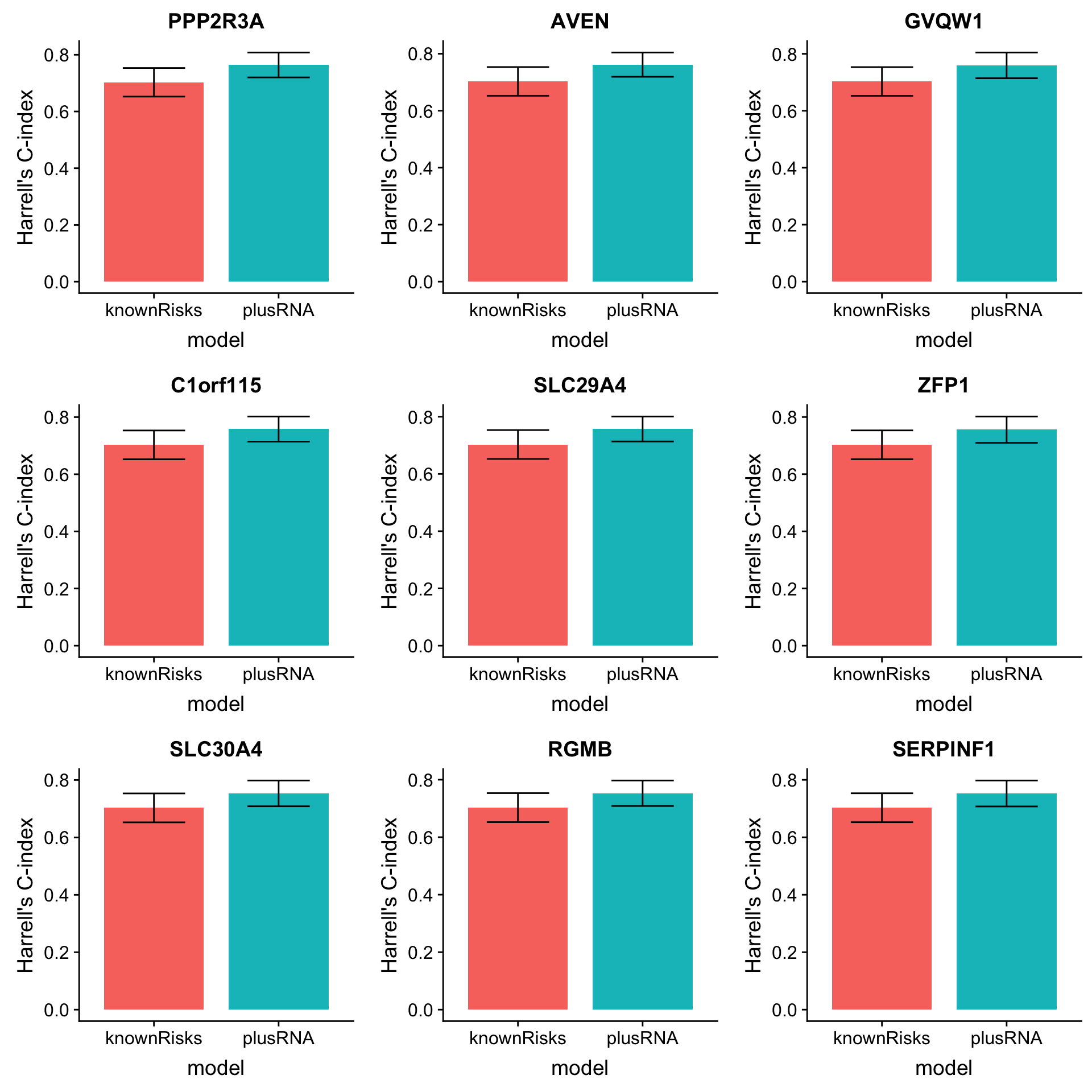
| Version | Author | Date |
|---|---|---|
| b8e0823 | Junyan Lu | 2020-03-10 |
OS
rnaMultiRes[["full"]][["OS"]] <- lapply(filter(rnaUniRes[["full"]][["OS"]], p<=0.05)$name, function(n) {
  risk0 <- riskTab.rna
  risk1 <- riskTab.rna %>% mutate(protExpr = rnaMat[n,patientID])
  res0 <- summary(runCox(survTab.rna, risk0, "OS","died"))
  res1 <- summary(runCox(survTab.rna, risk1, "OS","died"))
  tibble(name = n, c0 = res0$concordance[1], c1 = res1$concordance[1],
         se0 = res0$concordance[2],se1 = res1$concordance[2],
         ci0 = se0*1.96, ci1 = se1*1.96)
}) %>% bind_rows() %>% mutate(diffC = c1-c0) %>%
  arrange(desc(diffC))
Plot top 9 candidates
plotList <- lapply(1:9, function(i) {
  plotTab <- tibble(model = c("knownRisks","plusRNA"),
                    cindex = c(rnaMultiRes[["full"]][["OS"]][i,]$c0, rnaMultiRes[["full"]][["OS"]][i,]$c1),
                    ci = c(rnaMultiRes[["full"]][["OS"]][i,]$ci0,rnaMultiRes[["full"]][["OS"]][i,]$ci1))
  ggplot(plotTab, aes(x=model, y=cindex, fill = model)) +
    geom_bar(stat="identity",width=0.8) +
    geom_errorbar(aes(ymin=cindex + ci, ymax = cindex-ci), width=0.5) +
    ggtitle(rnaMultiRes[["full"]][["OS"]][i,]$name) + theme(legend.position = "none") +
    ylab("Harrell's C-index")
})
plot_grid(plotlist = plotList, ncol =3)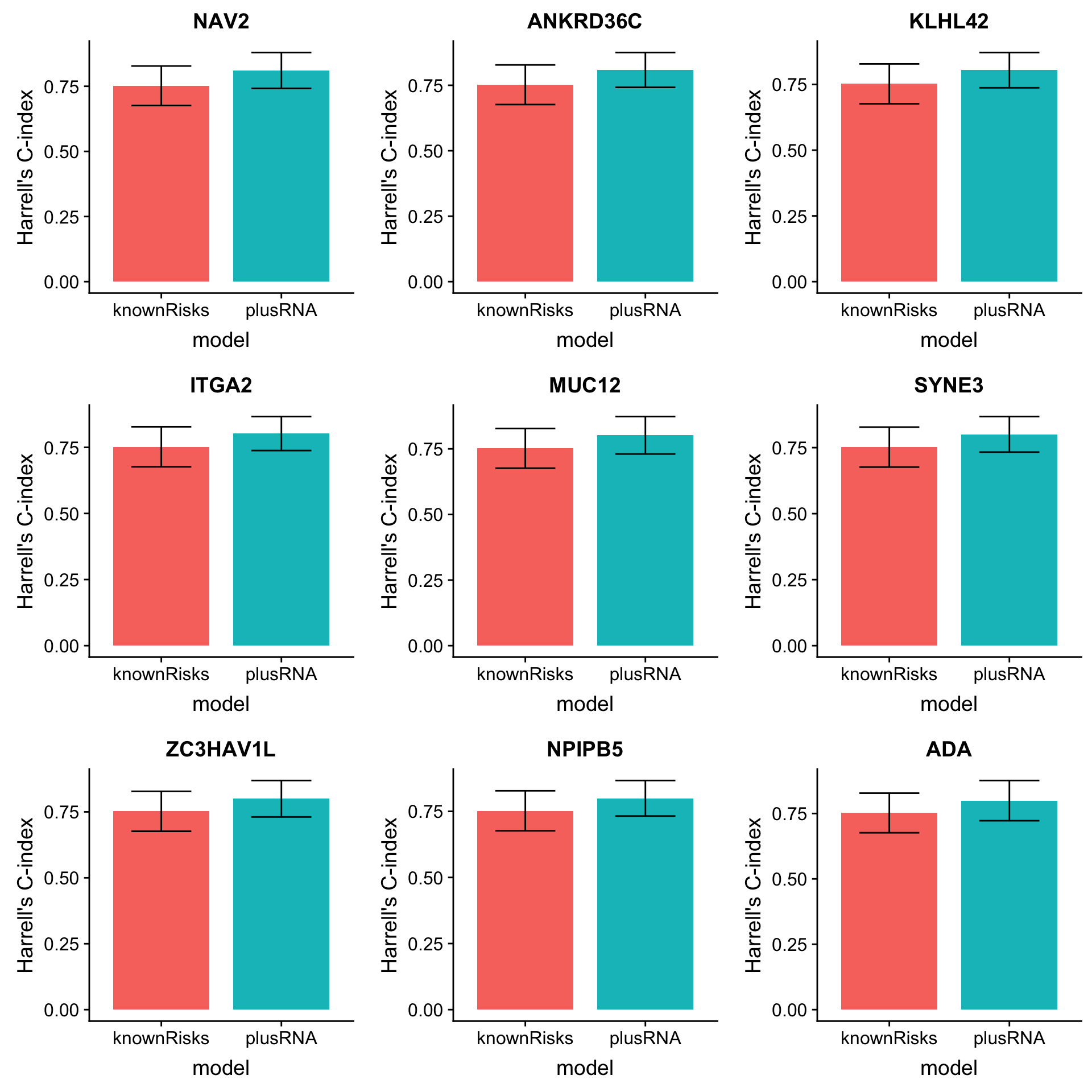
| Version | Author | Date |
|---|---|---|
| b8e0823 | Junyan Lu | 2020-03-10 |
Subsetted RNAseq dataset (samples also with proteomic data)
Univariate test
rnaMat <- rnaMat[,colnames(rnaMat) %in% colnames(protCLL)]
survTab.rna <- filter(survTab.rna, patientID %in% colnames(rnaMat))

rnaUniRes[["subset"]] <- list()

rnaUniRes[["subset"]][["TTT"]] <- lapply(rownames(rnaMat), function(n) {
  testTab <- mutate(survTab.rna, expr = rnaMat[n, patientID])
  com(testTab$expr, testTab$TTT, testTab$treatedAfter, TRUE) %>%
    mutate(name = n)
}) %>% bind_rows() %>% mutate(p.adj = p.adjust(p, method = "BH")) %>%
  arrange(p)

rnaUniRes[["subset"]][["OS"]] <- lapply(rownames(rnaMat), function(n) {
  testTab <- mutate(survTab.rna, expr = rnaMat[n, patientID])
  com(testTab$expr, testTab$OS, testTab$died, TRUE) %>%
    mutate(name = n)
}) %>% bind_rows() %>% mutate(p.adj = p.adjust(p, method = "BH")) %>%
  arrange(p)
P-value histogram
plotTab <- mutate(rnaUniRes$subset$TTT, outcome = "TTT") %>% bind_rows(mutate(rnaUniRes$subset$OS, outcome = "OS"))
ggplot(plotTab, aes(x=p, fill = outcome)) + geom_histogram(bins = 50) + facet_wrap(~outcome, scale = "free") +
  theme(legend.position = "none")+ xlim(0,1)
Warning: Removed 4 rows containing missing values (geom_bar).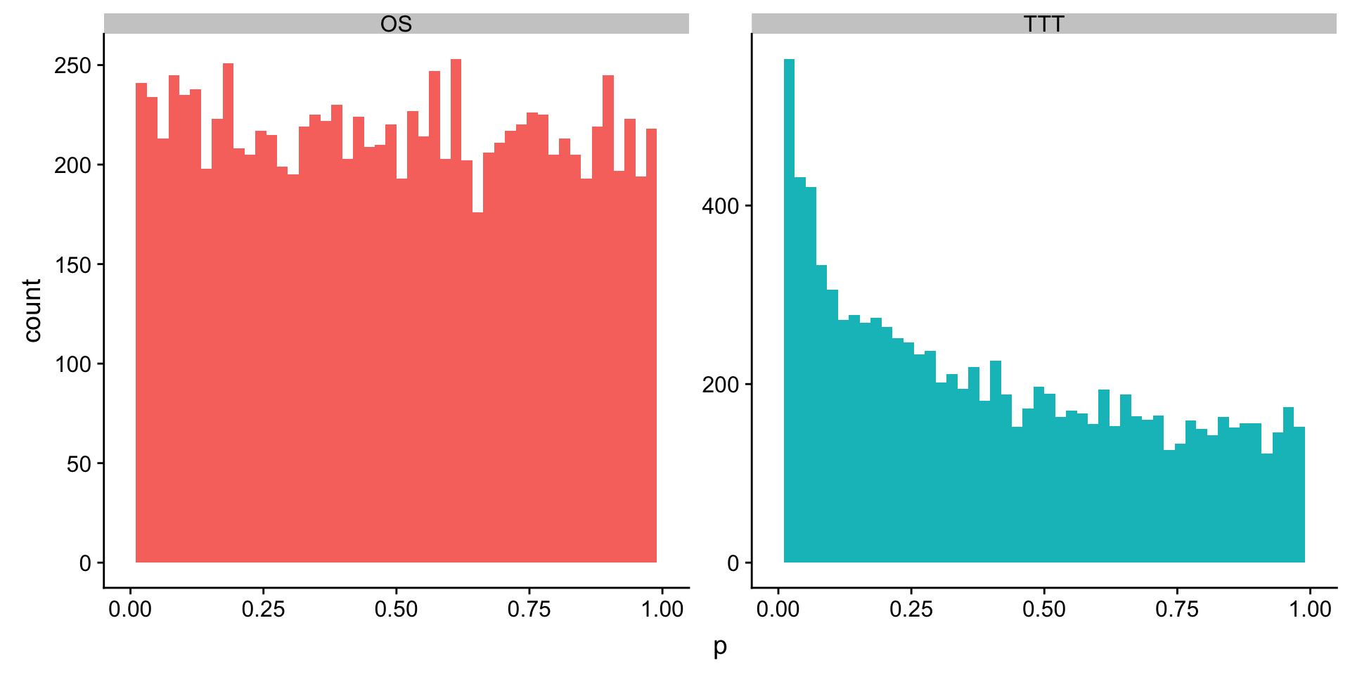
| Version | Author | Date |
|---|---|---|
| b8e0823 | Junyan Lu | 2020-03-10 |
Multi-variate model
Prepare table for known genomic risks
riskTab.rna <- select(survTab.rna, patientID, sampleID) %>%
  left_join(patMeta[,c("Patient.ID","IGHV.status","TP53","trisomy12","del17p","gender")], by = c(patientID = "Patient.ID")) %>%
  mutate(TP53 = as.numeric(as.character(TP53)),
         del17p = as.numeric(as.character(del17p))) %>%
  mutate(`TP53.del17p` = as.numeric(TP53 | del17p)) %>%
  select(-TP53, -del17p) %>%
  mutate_if(is.numeric, as.factor) %>%
  mutate(age = ageTab[match(sampleID, ageTab$sampleID),]$age) %>%
  dplyr::rename(sex=gender) %>%
  mutate(age = age/10) %>% select(-sampleID)
TTT
rnaMultiRes[["subset"]] <- list()

rnaMultiRes[["subset"]][["TTT"]] <- lapply(filter(rnaUniRes[["subset"]][["TTT"]], p<=0.05)$name, function(n) {
  risk0 <- riskTab.rna
  risk1 <- riskTab.rna %>% mutate(protExpr = rnaMat[n,patientID])
  res0 <- summary(runCox(survTab.rna, risk0, "TTT","treatedAfter"))
  res1 <- summary(runCox(survTab.rna, risk1, "TTT","treatedAfter"))
  tibble(name = n, c0 = res0$concordance[1], c1 = res1$concordance[1],
         se0 = res0$concordance[2],se1 = res1$concordance[2],
         ci0 = se0*1.96, ci1 = se1*1.96)
}) %>% bind_rows() %>% mutate(diffC = c1-c0) %>%
  arrange(desc(diffC))
Plot top 9 candidates
plotList <- lapply(1:9, function(i) {
  plotTab <- tibble(model = c("knownRisks","plusRNA"),
                    cindex = c(rnaMultiRes[["subset"]][["TTT"]][i,]$c0, rnaMultiRes[["subset"]][["TTT"]][i,]$c1),
                    ci = c(rnaMultiRes[["subset"]][["TTT"]][i,]$ci0,rnaMultiRes[["subset"]][["TTT"]][i,]$ci1))
  ggplot(plotTab, aes(x=model, y=cindex, fill = model)) +
    geom_bar(stat="identity",width=0.8) +
    geom_errorbar(aes(ymin=cindex + ci, ymax = cindex-ci), width=0.5) +
    ggtitle(rnaMultiRes[["subset"]][["TTT"]][i,]$name) + theme(legend.position = "none") +
    ylab("Harrell's C-index")
})
plot_grid(plotlist = plotList, ncol =3)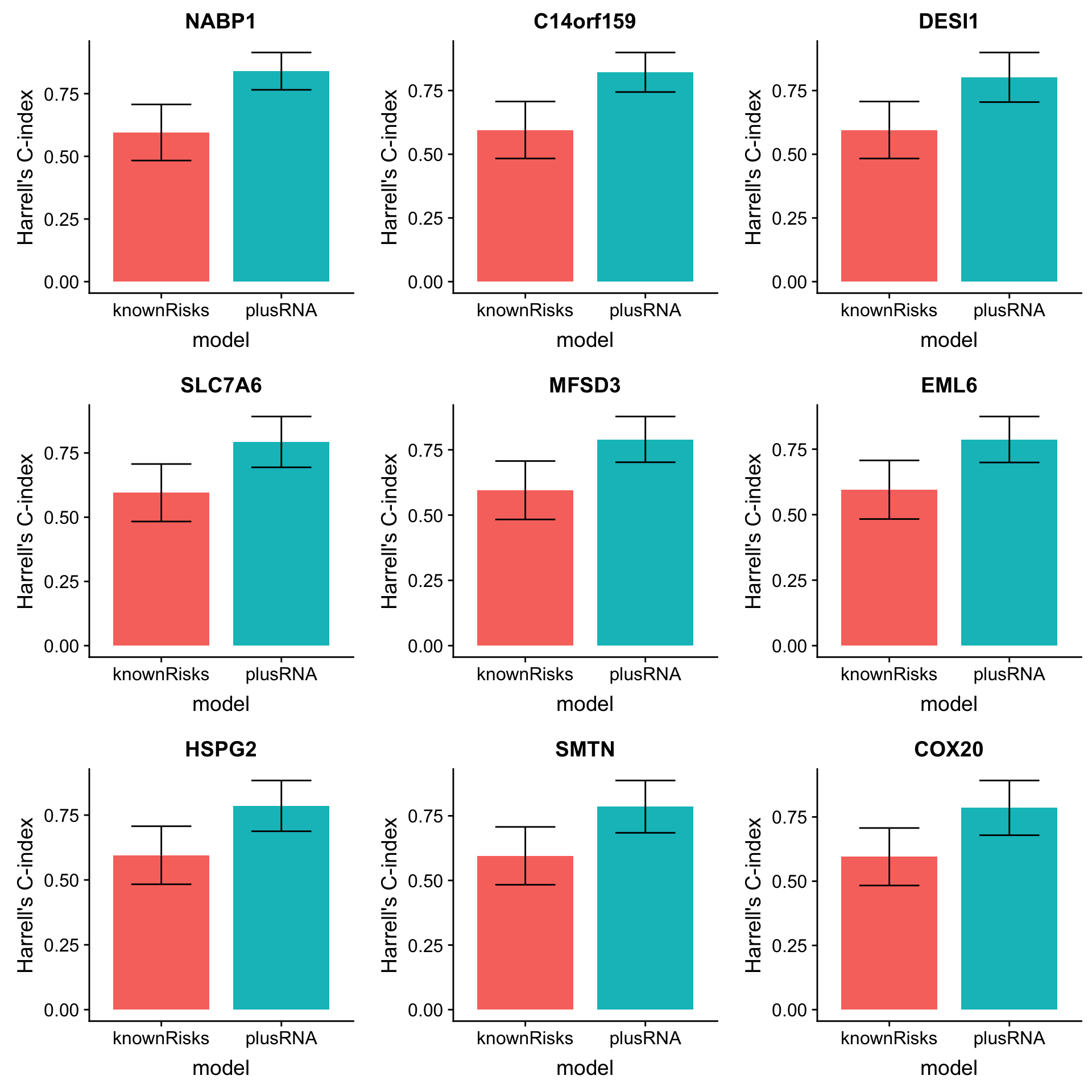
| Version | Author | Date |
|---|---|---|
| b8e0823 | Junyan Lu | 2020-03-10 |
OS
rnaMultiRes[["subset"]][["OS"]] <- lapply(filter(rnaUniRes[["subset"]][["OS"]], p<=0.05)$name, function(n) {
  tryCatch({
  risk0 <- riskTab.rna
  risk1 <- riskTab.rna %>% mutate(protExpr = rnaMat[n,patientID])
  res0 <- summary(runCox(survTab.rna, risk0, "OS","died"))
  res1 <- summary(runCox(survTab.rna, risk1, "OS","died"))
  tibble(name = n, c0 = res0$concordance[1], c1 = res1$concordance[1],
         se0 = res0$concordance[2],se1 = res1$concordance[2],
         ci0 = se0*1.96, ci1 = se1*1.96)
  }, error=function(cond) {
    tibble(name = NA, c0 = NA, c1 = NA,
         se0 = NA,se1 = NA,
         ci0 = se0*1.96, ci1 = se1*1.96)
  })
}) %>% bind_rows() %>% mutate(diffC = c1-c0) %>%
  arrange(desc(diffC))
Plot top 9 candidates
plotList <- lapply(1:9, function(i) {
  plotTab <- tibble(model = c("knownRisks","plusRNA"),
                    cindex = c(rnaMultiRes[["subset"]][["OS"]][i,]$c0, rnaMultiRes[["subset"]][["OS"]][i,]$c1),
                    ci = c(rnaMultiRes[["subset"]][["OS"]][i,]$ci0,rnaMultiRes[["subset"]][["OS"]][i,]$ci1))
  ggplot(plotTab, aes(x=model, y=cindex, fill = model)) +
    geom_bar(stat="identity",width=0.8) +
    geom_errorbar(aes(ymin=cindex + ci, ymax = cindex-ci), width=0.5) +
    ggtitle(rnaMultiRes[["subset"]][["OS"]][i,]$name) + theme(legend.position = "none") +
    ylab("Harrell's C-index")
})
plot_grid(plotlist = plotList, ncol =3)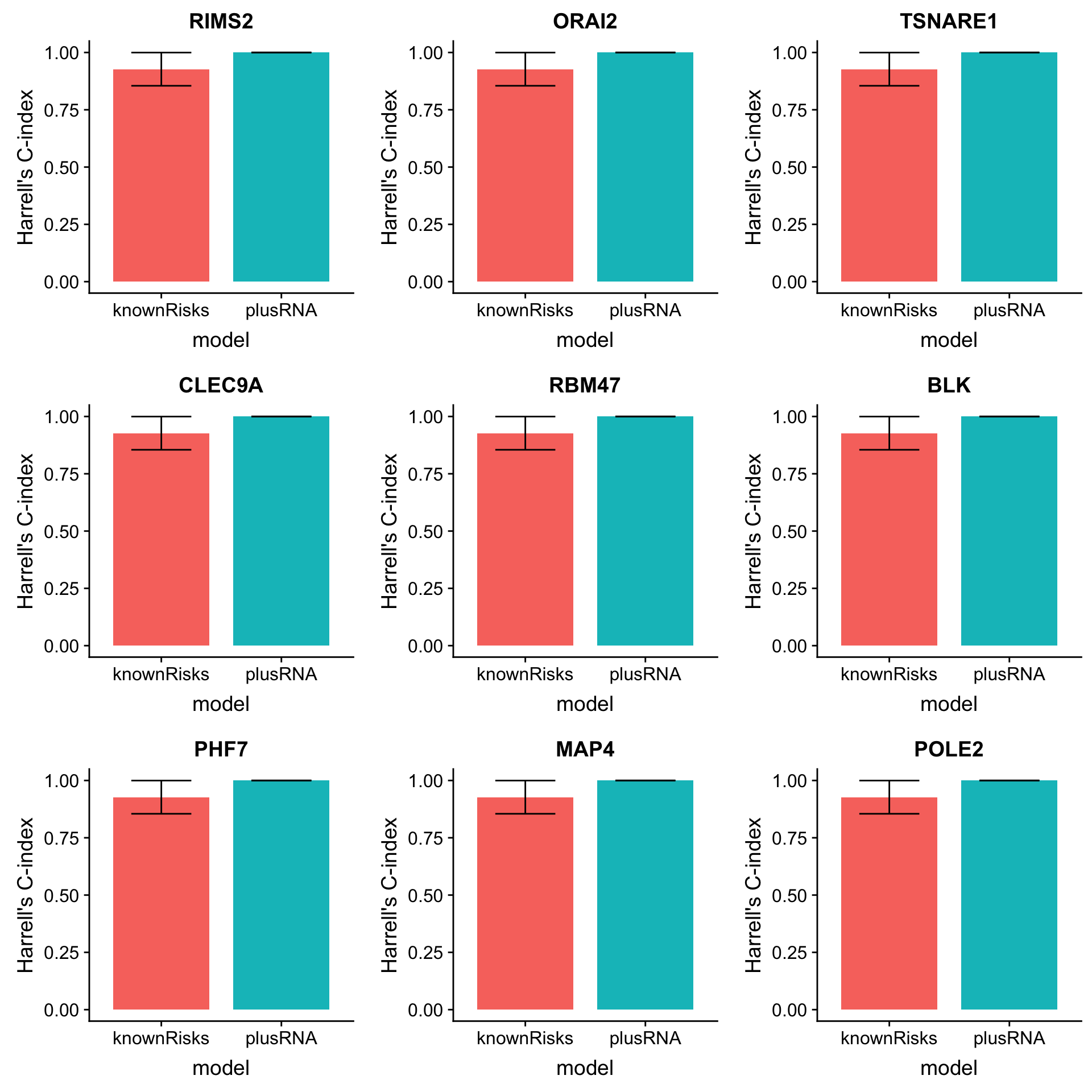
| Version | Author | Date |
|---|---|---|
| b8e0823 | Junyan Lu | 2020-03-10 |
Compare the C-index of RNAseq data and proteomics data for evaluating ability to predict outcomes
Overall comparison
TTT
plotTab.ttt <- bind_rows(select(cTab.ttt, name, diffC) %>% mutate(dataset = "Protein"),
                         select(rnaMultiRes$full$TTT, name, diffC) %>% mutate(dataset = "RNA_full"),
                         select(rnaMultiRes$subset$TTT, name, diffC) %>% mutate(dataset = "RNA_subset"))
ggplot(plotTab.ttt, aes(x=diffC, fill = dataset)) + geom_histogram(col = "grey50", alpha = 0.5, position = "identity")+
  xlab("Information gain to predict outcome")
`stat_bin()` using `bins = 30`. Pick better value with `binwidth`.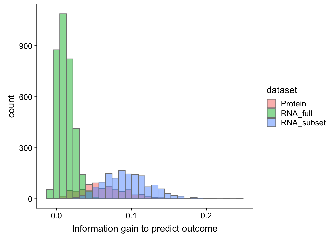
| Version | Author | Date |
|---|---|---|
| b8e0823 | Junyan Lu | 2020-03-10 |
OS
plotTab.os <- bind_rows(select(cTab.os, name, diffC) %>% mutate(dataset = "Protein"),
                         select(rnaMultiRes$full$OS, name, diffC) %>% mutate(dataset = "RNA_full"),
                         select(rnaMultiRes$subset$OS, name, diffC) %>% mutate(dataset = "RNA_subset"))
ggplot(plotTab.os, aes(x=diffC, fill = dataset)) + geom_histogram(col = "grey50", alpha = 0.5, position = "identity") +
  xlab("Information gain to predict outcome")
`stat_bin()` using `bins = 30`. Pick better value with `binwidth`.Warning: Removed 10 rows containing non-finite values (stat_bin).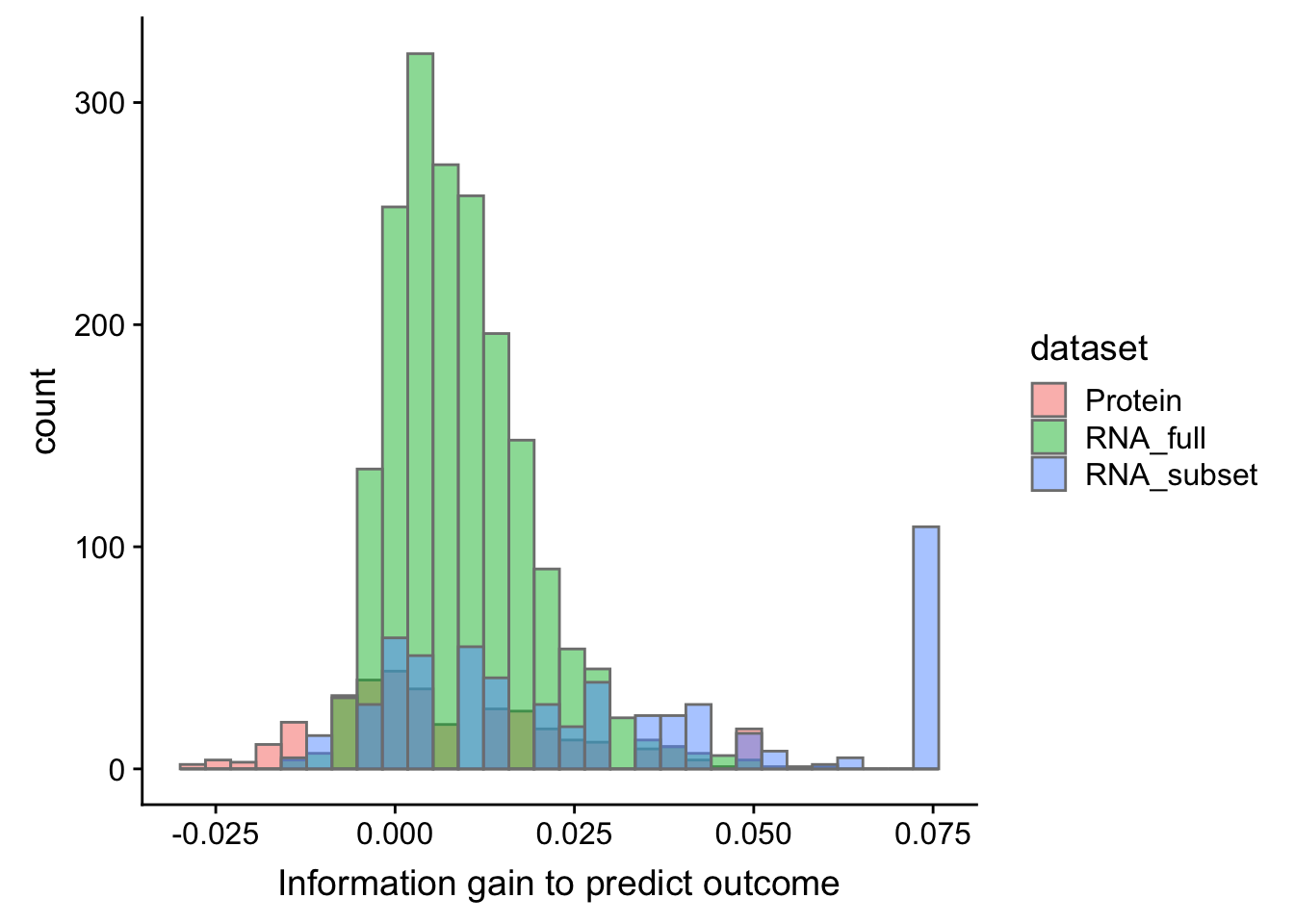
| Version | Author | Date |
|---|---|---|
| b8e0823 | Junyan Lu | 2020-03-10 |
Overall, proteomic dataset does not have advantage over RNAseq dataset for predicting outcome in multi-vairate model
For individual proteins
Re-do test for overlapped genes between RNAseq and proteomic datasets
Processing RNAseq data
ddsSub <- dds[,dds$diag %in% "CLL"]
ddsSub <- ddsSub[rowData(ddsSub)$symbol %in% rowData(protCLL)$hgnc_symbol,]
ddsSub <- ddsSub[rowSums(counts(ddsSub, normalized = TRUE)) > 10, ]
ddsSub.vst <- varianceStabilizingTransformation(ddsSub)
rnaMat <- assay(ddsSub.vst)
rownames(rnaMat) <- rowData(ddsSub.vst)$symbol
Prepare risk table
#table of known risks
survTab <- survT %>% filter(sampleID %in% ddsSub$sampleID) %>%
  select(patID,sampleID, OS, died, TTT, treatedAfter) %>%
  dplyr::rename(patientID = patID)

riskTab <- select(survTab, patientID, sampleID) %>%
  left_join(patMeta[,c("Patient.ID","IGHV.status","TP53","trisomy12","del17p","gender")], by = c(patientID = "Patient.ID")) %>%
  mutate(TP53 = as.numeric(as.character(TP53)),
         del17p = as.numeric(as.character(del17p))) %>%
  mutate(`TP53.del17p` = as.numeric(TP53 | del17p)) %>%
  select(-TP53, -del17p) %>%
  mutate_if(is.numeric, as.factor) %>%
  mutate(age = ageTab[match(sampleID, ageTab$sampleID),]$age) %>%
  dplyr::rename(sex=gender) %>%
  mutate(age = age/10) %>% select(-sampleID)
Information gain to predict TTT
Test if RNA expression also adds information
rnaTab.ttt <- lapply(filter(uniRes.ttt, p<=0.05)$name, function(n) {
  if (n %in% rownames(rnaMat)) {
  risk0 <- riskTab
  risk1 <- riskTab %>% mutate(protExpr = rnaMat[n,patientID])
  res0 <- summary(runCox(survTab, risk0, "TTT","treatedAfter"))
  res1 <- summary(runCox(survTab, risk1, "TTT","treatedAfter"))
  tibble(name = n, c0 = res0$concordance[1], c1 = res1$concordance[1],
         se0 = res0$concordance[2],se1 = res1$concordance[2],
         ci0 = se0*1.96, ci1 = se1*1.96)
  } else {
    tibble(id=n, c0 =NA, c1 = NA, se0 = NA, se1 = NA,
           ci0 = NA, ci1=NA)
  }

}) %>% bind_rows() %>% mutate(diffC = c1-c0) %>%
  arrange(desc(diffC)) %>%
  mutate(diffC = ifelse(is.na(diffC),0,diffC))
Compare with protein data
topList.ttt <- list(rna = arrange(rnaTab.ttt, desc(diffC))$name[1:20],
                      prot = arrange(cTab.ttt, desc(diffC))$name[1:20])

compareTab.ttt <- select(cTab.ttt, name, diffC) %>% dplyr::rename(diffProt = diffC) %>%
  left_join(select(rnaTab.ttt, name, diffC) %>% dplyr::rename(diffRNA = diffC)) %>%
  mutate(group = case_when(
    name %in% topList.ttt$rna & !name %in% topList.ttt$prot ~ "rnaOnly",
    name %in% topList.ttt$prot & !name %in% topList.ttt$rna ~ "proteinOnly",
    name %in% topList.ttt$rna & name %in% topList.ttt$prot ~ "both",
    TRUE ~ "none"
  ))
Joining, by = "name"ggplot(compareTab.ttt, aes(x=diffProt, y =diffRNA)) + geom_point(aes(col = group)) +
ggrepel::geom_text_repel(data = filter(compareTab.ttt, group != "none"), aes(label = name)) +
scale_color_manual(values = c(rnaOnly = "green", proteinOnly = "blue", both = "red", none = "grey50")) +
ylab("Information gain by including RNA expression") +
xlab("Information gain by including protein expression")Warning: Removed 24 rows containing missing values (geom_point).Warning: Removed 1 rows containing missing values (geom_text_repel).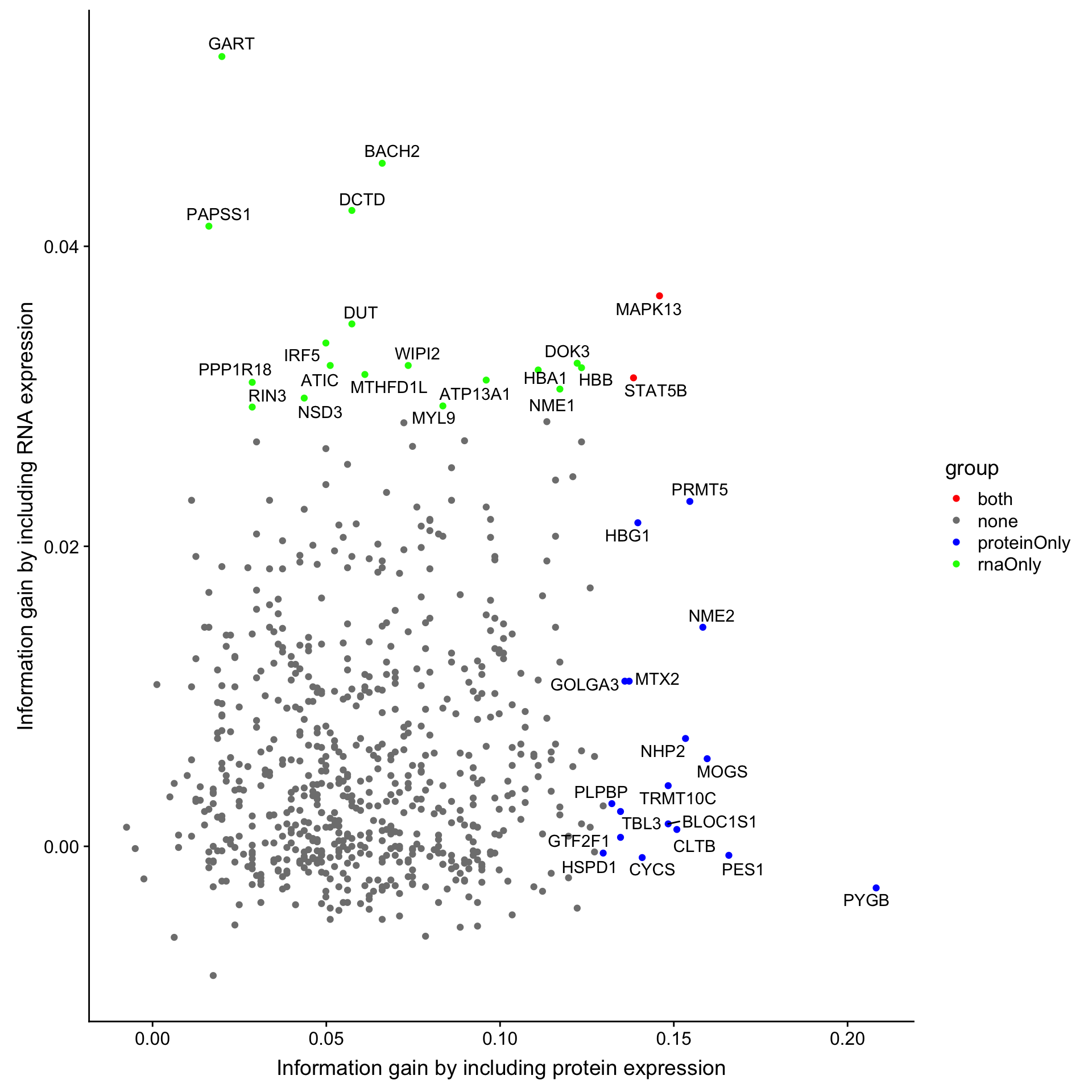
| Version | Author | Date |
|---|---|---|
| b8e0823 | Junyan Lu | 2020-03-10 |
Top 20 RNA candidates are colored by greed. Top 20 protein candidates are colored by red. Overlapped candidates are colored by red.
Information gain to predict OS
Test if RNA expression also adds information
rnaTab.os <- lapply(filter(uniRes.os, p<=0.05)$name, function(n) {
  if (n %in% rownames(rnaMat)) {
  risk0 <- riskTab
  risk1 <- riskTab %>% mutate(protExpr = rnaMat[n,patientID])
  res0 <- summary(runCox(survTab, risk0, "OS","died"))
  res1 <- summary(runCox(survTab, risk1, "OS","died"))
  tibble(name = n, c0 = res0$concordance[1], c1 = res1$concordance[1],
         se0 = res0$concordance[2],se1 = res1$concordance[2],
         ci0 = se0*1.96, ci1 = se1*1.96)
  } else {
    tibble(id=n, c0 =NA, c1 = NA, se0 = NA, se1 = NA,
           ci0 = NA, ci1=NA)
  }

}) %>% bind_rows() %>% mutate(diffC = c1-c0) %>%
  arrange(desc(diffC)) %>%
  mutate(diffC = ifelse(is.na(diffC),0,diffC))
Compare with protein data
topList.os <- list(rna = arrange(rnaTab.os, desc(diffC))$name[1:20],
                      prot = arrange(cTab.os, desc(diffC))$name[1:20])

compareTab.os <- select(cTab.os, name, diffC) %>% dplyr::rename(diffProt = diffC) %>%
  left_join(select(rnaTab.os, name, diffC) %>% dplyr::rename(diffRNA = diffC)) %>%
  mutate(group = case_when(
    name %in% topList.os$rna & !name %in% topList.os$prot ~ "rnaOnly",
    name %in% topList.os$prot & !name %in% topList.os$rna ~ "proteinOnly",
    name %in% topList.os$rna & name %in% topList.os$prot ~ "both",
    TRUE ~ "none"
  ))
Joining, by = "name"ggplot(compareTab.os, aes(x=diffProt, y =diffRNA)) + geom_point(aes(col = group)) +
ggrepel::geom_text_repel(data = filter(compareTab.os, group != "none"), aes(label = name)) +
scale_color_manual(values = c(rnaOnly = "green", proteinOnly = "blue", both = "red", none = "grey50")) +
ylab("Information gain by including RNA expression") +
xlab("Information gain by including protein expression")Warning: Removed 6 rows containing missing values (geom_point).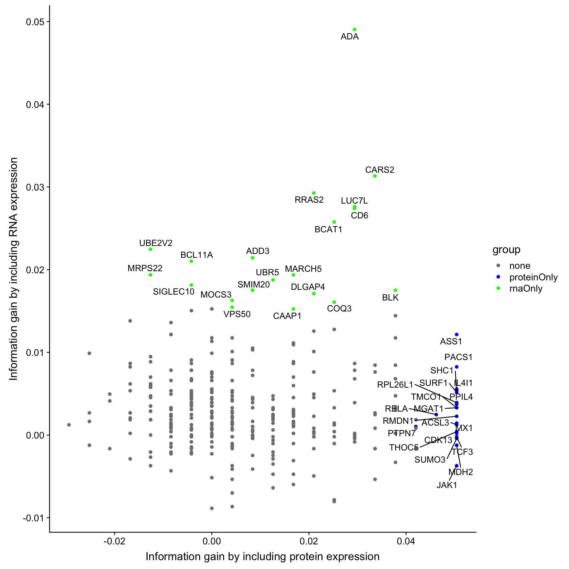
| Version | Author | Date |
|---|---|---|
| b8e0823 | Junyan Lu | 2020-03-10 |
Top 20 RNA candidates are colored by greed. Top 20 protein candidates are colored by red. Overlapped candidates are colored by red.
sessionInfo()R version 3.6.0 (2019-04-26)
Platform: x86_64-apple-darwin15.6.0 (64-bit)
Running under: macOS 10.15.4
Matrix products: default
BLAS: /Library/Frameworks/R.framework/Versions/3.6/Resources/lib/libRblas.0.dylib
LAPACK: /Library/Frameworks/R.framework/Versions/3.6/Resources/lib/libRlapack.dylib
locale:
[1] en_US.UTF-8/en_US.UTF-8/en_US.UTF-8/C/en_US.UTF-8/en_US.UTF-8
attached base packages:
[1] parallel stats4 stats graphics grDevices utils datasets
[8] methods base
other attached packages:
[1] latex2exp_0.4.0 forcats_0.4.0
[3] stringr_1.4.0 dplyr_0.8.5
[5] purrr_0.3.3 readr_1.3.1
[7] tidyr_1.0.0 tibble_3.0.0
[9] tidyverse_1.3.0 DESeq2_1.24.0
[11] SummarizedExperiment_1.14.0 DelayedArray_0.10.0
[13] BiocParallel_1.18.0 matrixStats_0.54.0
[15] Biobase_2.44.0 GenomicRanges_1.36.0
[17] GenomeInfoDb_1.20.0 IRanges_2.18.1
[19] S4Vectors_0.22.0 BiocGenerics_0.30.0
[21] maxstat_0.7-25 glmnet_2.0-18
[23] foreach_1.4.4 Matrix_1.2-17
[25] survminer_0.4.4 ggpubr_0.2.1
[27] magrittr_1.5 survival_2.44-1.1
[29] jyluMisc_0.1.5 pheatmap_1.0.12
[31] cowplot_0.9.4 ggplot2_3.3.0
[33] limma_3.40.2
loaded via a namespace (and not attached):
[1] utf8_1.1.4 shinydashboard_0.7.1 tidyselect_1.0.0
[4] RSQLite_2.1.1 AnnotationDbi_1.46.0 htmlwidgets_1.3
[7] grid_3.6.0 munsell_0.5.0 codetools_0.2-16
[10] DT_0.7 withr_2.1.2 colorspace_1.4-1
[13] knitr_1.23 rstudioapi_0.10 ggsignif_0.5.0
[16] labeling_0.3 git2r_0.26.1 slam_0.1-45
[19] GenomeInfoDbData_1.2.1 KMsurv_0.1-5 bit64_0.9-7
[22] farver_2.0.3 rprojroot_1.3-2 vctrs_0.2.4
[25] generics_0.0.2 TH.data_1.0-10 xfun_0.8
[28] sets_1.0-18 R6_2.4.0 locfit_1.5-9.1
[31] bitops_1.0-6 fgsea_1.10.0 assertthat_0.2.1
[34] promises_1.0.1 scales_1.1.0 multcomp_1.4-10
[37] nnet_7.3-12 gtable_0.3.0 sandwich_2.5-1
[40] workflowr_1.6.0 rlang_0.4.5 genefilter_1.66.0
[43] cmprsk_2.2-8 splines_3.6.0 acepack_1.4.1
[46] broom_0.5.2 checkmate_2.0.0 yaml_2.2.0
[49] abind_1.4-5 modelr_0.1.5 crosstalk_1.0.0
[52] backports_1.1.4 httpuv_1.5.1 Hmisc_4.2-0
[55] tools_3.6.0 relations_0.6-8 ellipsis_0.2.0
[58] gplots_3.0.1.1 RColorBrewer_1.1-2 Rcpp_1.0.1
[61] base64enc_0.1-3 visNetwork_2.0.7 zlibbioc_1.30.0
[64] RCurl_1.95-4.12 rpart_4.1-15 zoo_1.8-6
[67] ggrepel_0.8.1 haven_2.2.0 cluster_2.1.0
[70] exactRankTests_0.8-30 fs_1.4.0 data.table_1.12.2
[73] openxlsx_4.1.0.1 reprex_0.3.0 mvtnorm_1.0-11
[76] whisker_0.3-2 hms_0.5.2 shinyjs_1.0
[79] mime_0.7 evaluate_0.14 xtable_1.8-4
[82] XML_3.98-1.20 rio_0.5.16 readxl_1.3.1
[85] gridExtra_2.3 compiler_3.6.0 KernSmooth_2.23-15
[88] crayon_1.3.4 htmltools_0.4.0 later_0.8.0
[91] Formula_1.2-3 geneplotter_1.62.0 lubridate_1.7.4
[94] DBI_1.0.0 dbplyr_1.4.2 MASS_7.3-51.4
[97] car_3.0-3 cli_1.1.0 marray_1.62.0
[100] gdata_2.18.0 igraph_1.2.4.1 pkgconfig_2.0.2
[103] km.ci_0.5-2 foreign_0.8-71 piano_2.0.2
[106] xml2_1.2.2 annotate_1.62.0 XVector_0.24.0
[109] drc_3.0-1 rvest_0.3.5 digest_0.6.19
[112] rmarkdown_1.13 cellranger_1.1.0 fastmatch_1.1-0
[115] survMisc_0.5.5 htmlTable_1.13.1 curl_3.3
[118] shiny_1.3.2 gtools_3.8.1 lifecycle_0.2.0
[121] nlme_3.1-140 jsonlite_1.6 carData_3.0-2
[124] fansi_0.4.0 pillar_1.4.3 lattice_0.20-38
[127] httr_1.4.1 plotrix_3.7-6 glue_1.3.2
[130] zip_2.0.2 iterators_1.0.10 bit_1.1-14
[133] stringi_1.4.3 blob_1.1.1 latticeExtra_0.6-28
[136] caTools_1.17.1.2 memoise_1.1.0