Raw data processing of the proteomic data from timsTOF machine
Junyan Lu
2020-02-27
Last updated: 2020-03-10
Checks: 7 0
Knit directory: Proteomics/analysis/
This reproducible R Markdown analysis was created with workflowr (version 1.6.0). The Checks tab describes the reproducibility checks that were applied when the results were created. The Past versions tab lists the development history.
Great! Since the R Markdown file has been committed to the Git repository, you know the exact version of the code that produced these results.
Great job! The global environment was empty. Objects defined in the global environment can affect the analysis in your R Markdown file in unknown ways. For reproduciblity it’s best to always run the code in an empty environment.
The command set.seed(20200227) was run prior to running the code in the R Markdown file. Setting a seed ensures that any results that rely on randomness, e.g. subsampling or permutations, are reproducible.
Great job! Recording the operating system, R version, and package versions is critical for reproducibility.
Nice! There were no cached chunks for this analysis, so you can be confident that you successfully produced the results during this run.
Great job! Using relative paths to the files within your workflowr project makes it easier to run your code on other machines.
Great! You are using Git for version control. Tracking code development and connecting the code version to the results is critical for reproducibility. The version displayed above was the version of the Git repository at the time these results were generated.
Note that you need to be careful to ensure that all relevant files for the analysis have been committed to Git prior to generating the results (you can use wflow_publish or wflow_git_commit). workflowr only checks the R Markdown file, but you know if there are other scripts or data files that it depends on. Below is the status of the Git repository when the results were generated:
Ignored files:
    Ignored:    .DS_Store
    Ignored:    .Rhistory
    Ignored:    .Rproj.user/
    Ignored:    analysis/.DS_Store
    Ignored:    analysis/.Rhistory
    Ignored:    analysis/compareProteomicsRNAseq_cache/
    Ignored:    analysis/correlateCLLPD_cache/
    Ignored:    analysis/correlateGenomic_cache/
    Ignored:    analysis/correlateGenomic_removePC_cache/
    Ignored:    analysis/correlateMIR_cache/
    Ignored:    analysis/correlateMethylationCluster_cache/
    Ignored:    analysis/predictOutcome_cache/
    Ignored:    data/.DS_Store
    Ignored:    output/.DS_Store

Untracked files:
    Untracked:  code/utils.R
    Untracked:  data/190909_CLL_prot_abund_med_norm.tsv
    Untracked:  data/190909_CLL_prot_abund_no_norm.tsv
    Untracked:  data/20190423_Proteom_submitted_samples_bereinigt.xlsx
    Untracked:  data/20191025_Proteom_submitted_samples_final.xlsx
    Untracked:  data/LUMOS/
    Untracked:  data/LUMOS_peptides/
    Untracked:  data/LUMOS_protAnnotation.csv
    Untracked:  data/SampleAnnotation_cleaned.xlsx
    Untracked:  data/facTab_IC50atLeast3New.RData
    Untracked:  data/gmts/
    Untracked:  data/mapEnsemble.txt
    Untracked:  data/mapSymbol.txt
    Untracked:  data/pyprophet_export_aligned.csv
    Untracked:  data/timsTOF_protAnnotation.csv
    Untracked:  output/LUMOS_processed.RData
    Untracked:  output/proteomic_LUMOS_20200227.RData
    Untracked:  output/proteomic_timsTOF_20200227.RData
    Untracked:  output/timsTOF_processed.RData
Note that any generated files, e.g. HTML, png, CSS, etc., are not included in this status report because it is ok for generated content to have uncommitted changes.
These are the previous versions of the R Markdown and HTML files. If you’ve configured a remote Git repository (see ?wflow_git_remote), click on the hyperlinks in the table below to view them.
| File | Version | Author | Date | Message |
|---|---|---|---|---|
| html | 46534c2 | Junyan Lu | 2020-02-27 | Build site. |
| Rmd | 2b8852e | Junyan Lu | 2020-02-27 | wflow_publish(list.files(“./”, pattern = “Rmd”)) |
| html | cc8c163 | Junyan Lu | 2020-02-27 | Build site. |
| Rmd | 16c2694 | Junyan Lu | 2020-02-27 | wflow_publish(c(“processProteomics_LUMOS.Rmd”, “index.Rmd”, |
Date input
Read and annotate data
Read in data and annotate raw data (unnormalized)
rawTab <- read_tsv("../data/190909_CLL_prot_abund_no_norm.tsv") %>%
  separate(X1, c("sp","uniprotID","name","hm"), sep = "[|_]") %>%
  select(-sp, -hm) %>%
  gather(key = "id",value = "count",-uniprotID, -name) %>%
  mutate(ID = uniprotID)

#annotate patient ID
patAnno <- readxl::read_xlsx("../data/SampleAnnotation_cleaned.xlsx") %>%
  mutate(id = paste0("A_1_",id)) %>%
  select(-Institute, -Source, -diagnosis)

#annotate basic genomic feature
genAnno <- patMeta %>% select(Patient.ID, gender, IGHV.status, trisomy12) %>%
  mutate(trisomy12 = as.integer(as.character(trisomy12))) %>%
  mutate(trisomy12 = ifelse(Patient.ID == "P0494",1,trisomy12)) %>%
  mutate(trisomy12 = factor(trisomy12))


#annotate technical variable
techTab <- readxl::read_xlsx("../data/20191025_Proteom_submitted_samples_final.xlsx") %>%
  select(`Patient ID`, operator, viability, batch, `date of sample processing`, `protein conc. in ug`, `freeze-thaw cycles of peptide solution`) %>% dplyr::rename(patID = `Patient ID`, processDate = `date of sample processing`, proteinConc = `protein conc. in ug`, `freeThawCycle` = `freeze-thaw cycles of peptide solution`) %>%
  mutate(batch = ifelse(batch == "test run", "0", batch))

patAnno <- left_join(patAnno, genAnno, by = c(patID = "Patient.ID")) %>%
  left_join(techTab, by = "patID")

rawTab <- left_join(rawTab, patAnno, by = "id")
Create SummarizedExperiment object
protCLL <- tidyToSum(rawTab, "uniprotID", "patID", "count",
                     annoCol = colnames(patAnno)[colnames(patAnno) != "patID"],
                     annoRow = c("name","ID"))
Dimension of the original data
dim(protCLL)[1] 3942 49Annotate protein information using bioMart
Find annotations use uniprot ID
#firstly based on id
ids <- rowData(protCLL)$ID


ensembl = useMart("ensembl",dataset="hsapiens_gene_ensembl")
anno <- getBM(attributes=c('uniprot_gn_symbol','ensembl_gene_id', 'hgnc_symbol','chromosome_name','uniprotswissprot'),
      filters = 'uniprotswissprot',
      values = ids,
      mart = ensembl)
annoUnique <- filter(anno, !grepl("CHR",chromosome_name)) %>% distinct(uniprotswissprot, .keep_all = TRUE)

rowAnno <- rowData(protCLL) %>% data.frame(stringsAsFactors = FALSE) %>%
  left_join(annoUnique, by = c(ID  = "uniprotswissprot"))

missAnno <- filter(rowAnno, is.na(ensembl_gene_id))
#For how many proteins the annotation can not be retrieved by uniprot id mapping?
nrow(missAnno)
Try annotate by gene symbol
ids <- missAnno$name
annoName <- getBM(attributes=c('uniprot_gn_symbol','ensembl_gene_id', 'hgnc_symbol','chromosome_name','uniprotswissprot'),
      filters = 'hgnc_symbol',
      values = ids,
      mart = ensembl)
annoNameUnique <- filter(annoName, !grepl("CHR",chromosome_name)) %>% distinct(hgnc_symbol, .keep_all = TRUE)
rowAnno[match(annoNameUnique$hgnc_symbol, rowAnno$name),3:6] <- annoNameUnique[,1:4]

missAnno <- filter(rowAnno, is.na(ensembl_gene_id))
#For how many proteins the annotation can not be retrieved by uniprot id mapping?
nrow(missAnno)
Annotate
rowAnno <- column_to_rownames(rowAnno, "ID")
rowData(protCLL) <- rowAnno
rowData(protCLL)$ID <- rownames(protCLL)
Save the annotation in a csv table
write_csv2(data.frame(rowData(protCLL)),"../data/timsTOF_protAnnotation.csv")Annotate using saved annotation table (bioMart takes long time)
annoTab <- read_csv2("../data/timsTOF_protAnnotation.csv") %>%
  data.frame(stringsAsFactors = FALSE)
Using ',' as decimal and '.' as grouping mark. Use read_delim() for more control.Parsed with column specification:
cols(
name = col_character(),
uniprot_gn_symbol = col_character(),
ensembl_gene_id = col_character(),
hgnc_symbol = col_character(),
chromosome_name = col_character(),
ID = col_character()
)rowData(protCLL) <- annoTab[match(rownames(protCLL),annoTab$ID),]Below proteins in the proteomic dataset can not be annotated by using bioMart, therefore their corresponding ensemble gene ID can not be determined.
annoTab[is.na(annoTab$ensembl_gene_id),] %>% select(name, ID) name ID
34 NCF1B A6NI72
49 YS060 I3L1I5
495 PR40A O75400
780 1A68 P01891
781 1A02 P01892
782 HLAH P01893
785 DQB1 P01920
823 1C03 P04222
862 1A24 P05534
1078 2B14 P13760
1079 2B17 P13761
1080 DRB4 P13762
1101 CX7A2 P14406
1234 2B1B P20039
1423 ES1 P30042
1443 1B41 P30479
1444 1B44 P30481
1445 1B47 P30485
1446 1C02 P30501
1447 1C04 P30504
1455 GSTT1 P30711
2578 PM2PB Q13670
2934 2B18 Q30134
2935 2B1A Q30167
3020 H90B4 Q58FF6
3021 H90B2 Q58FF8
3038 RS26L Q5JNZ5
3094 GPTC4 Q5T3I0
3161 RN213 Q63HN8
3376 YJ005 Q6ZSR9
3380 E400N Q6ZTU2
3546 ZN598 Q86UK7
3560 THOC4 Q86V81
3938 LIRB1 Q8NHL6Initial QA
Check distribution of missing values
Pattern of missing values
plot_missval(protCLL)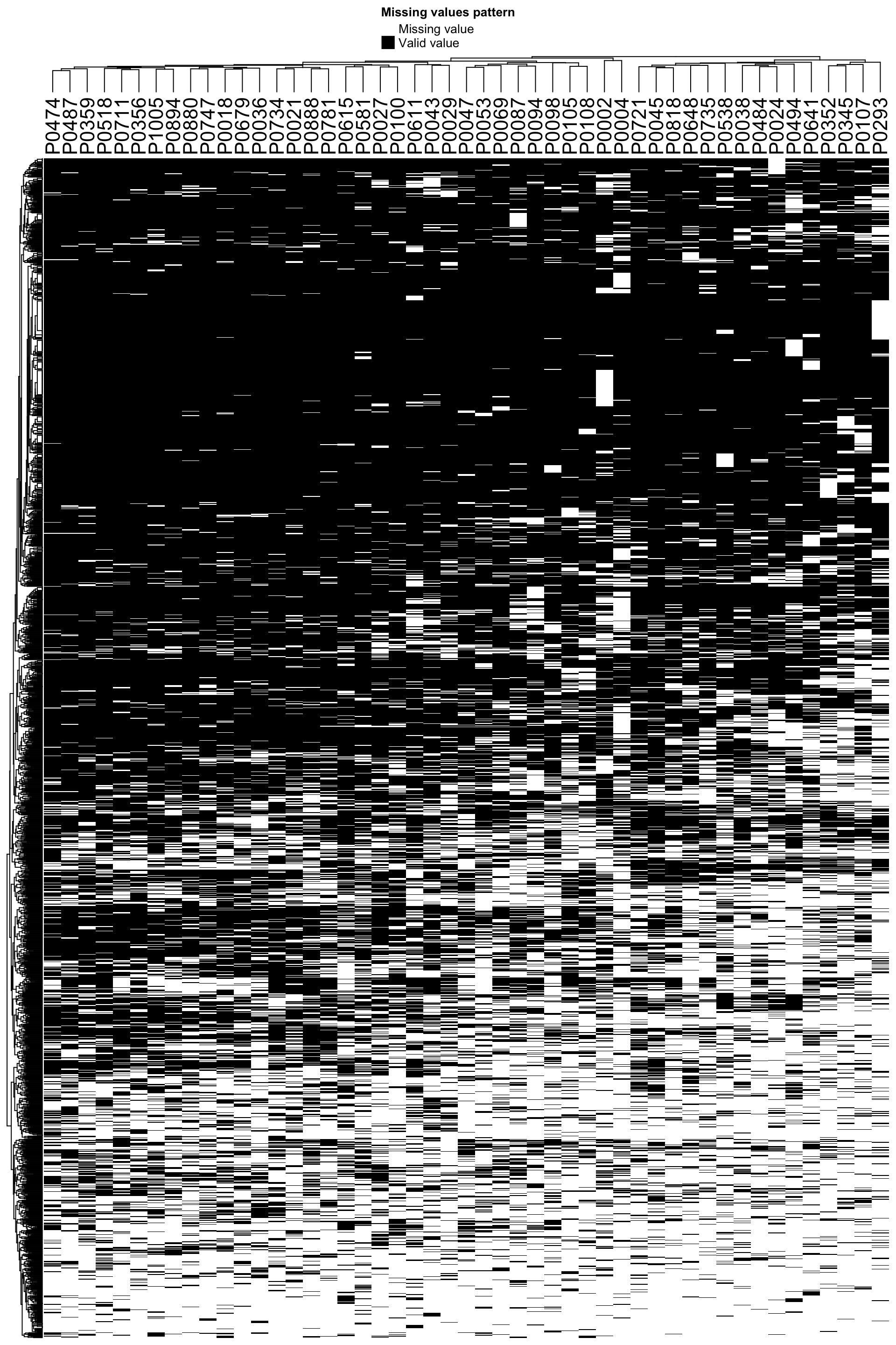
| Version | Author | Date |
|---|---|---|
| cc8c163 | Junyan Lu | 2020-02-27 |
Some samples show less detection rate than others.
Frequencies of missing values for each sample
proTab <- sumToTiday(protCLL, "uniprotID", "patientID")
patMiss <- group_by(proTab, patientID) %>%
  summarise(freqNA = sum(is.na(count))/length(count)) %>%
  arrange(desc(freqNA)) %>%
  mutate(patientID = factor(patientID, levels = patientID))

ggplot(patMiss, aes(x = patientID, y = freqNA)) + geom_point(size=3) +
  geom_segment(aes(x=patientID, xend=patientID, y=0, yend=freqNA)) +
  theme(axis.text.x = element_text(angle = 90, vjust =0.5, hjust=1)) + ylab("Frenquency")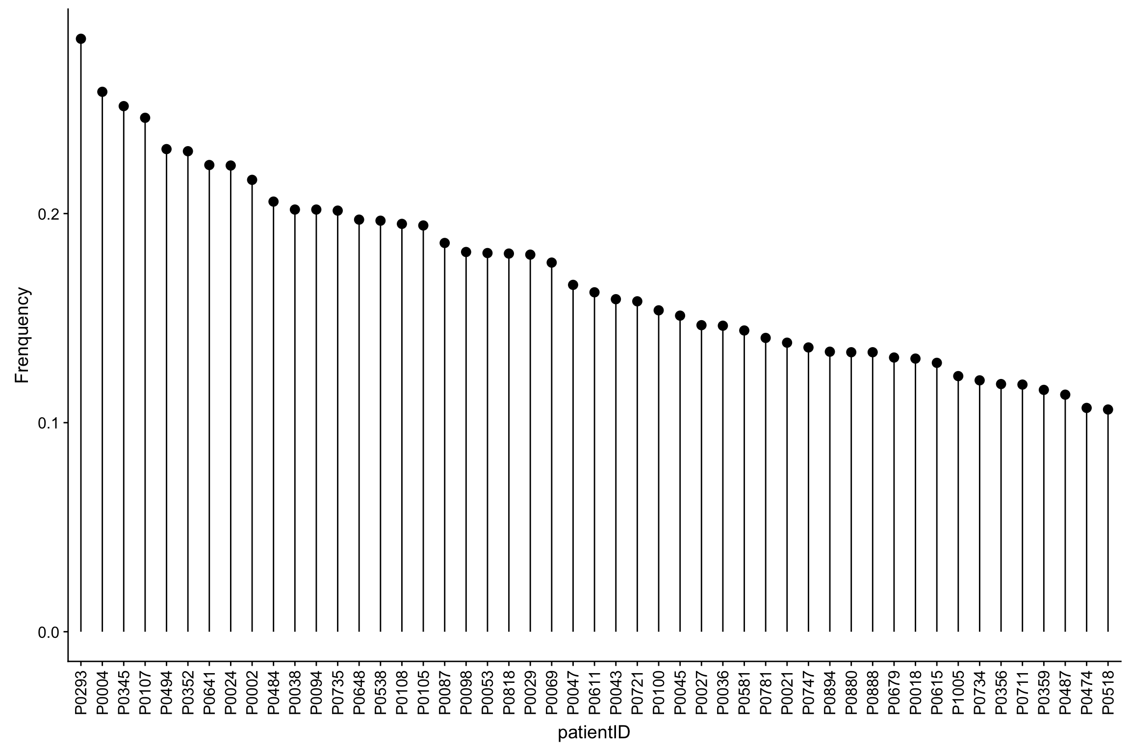
| Version | Author | Date |
|---|---|---|
| cc8c163 | Junyan Lu | 2020-02-27 |
All samples have relatively high detection rate (>70% proteins can be detected).
Proteins with missing values
proMiss <- group_by(proTab, name) %>%
  summarise(freqNA = sum(is.na(count))/length(count)) %>%
  arrange(desc(freqNA)) %>%
  mutate(name = factor(name, levels = name))

head(proMiss)
# A tibble: 6 x 2
name freqNA
<fct> <dbl>
1 2B1A 0.980
2 AL1L2 0.980
3 ARHG5 0.980
4 ASPH 0.980
5 BCL7A 0.980
6 C1QC 0.980ggplot(proMiss, aes(x=freqNA)) + geom_histogram() +
xlab("Missing value frequency")`stat_bin()` using `bins = 30`. Pick better value with `binwidth`.
| Version | Author | Date |
|---|---|---|
| cc8c163 | Junyan Lu | 2020-02-27 |
Missing value cut-off versus number of remaining proteins
sumTab <- lapply(seq(0,1,by = 0.01), function(x) tibble(cut = x, freq = sum(proMiss$freqNA < x)/nrow(proMiss))) %>% bind_rows()
ggplot(sumTab, aes(x=cut, y=freq)) + geom_line() + xlab("Missing value cut-off") + ylab("Percent remaining")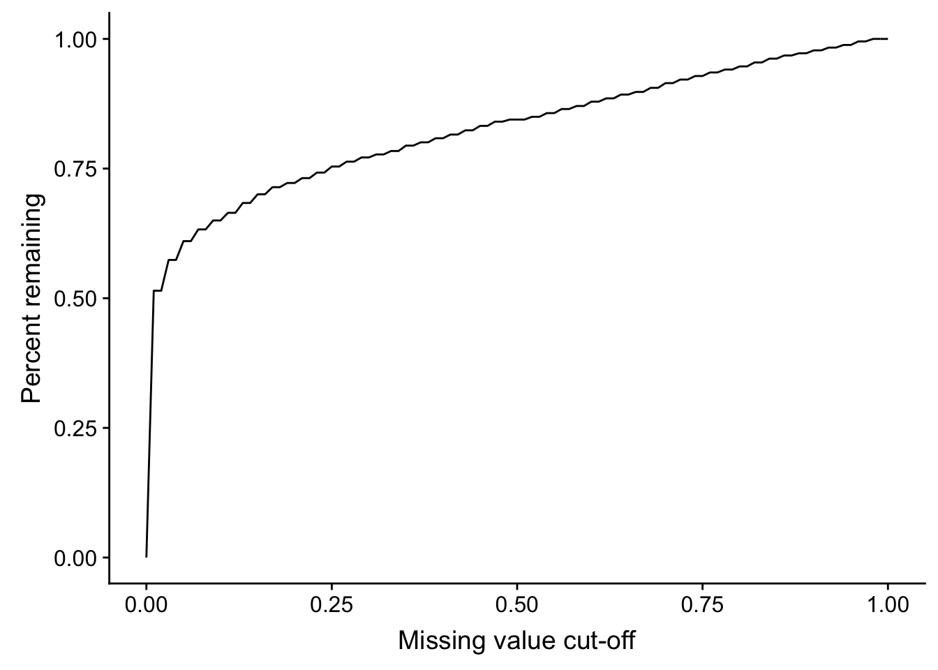
| Version | Author | Date |
|---|---|---|
| cc8c163 | Junyan Lu | 2020-02-27 |
Missing value frequency versus median expression
compareTab <- group_by(proTab, name) %>%
  summarise(freqNA = sum(is.na(count))/length(count),
            medianExpr = median(log2(count), na.rm=TRUE))

ggplot(compareTab, aes(x=freqNA, y = medianExpr)) + geom_point() + geom_smooth(method = "loess") +
  ylab("Median log2 count") + xlab("Frequency of missing values")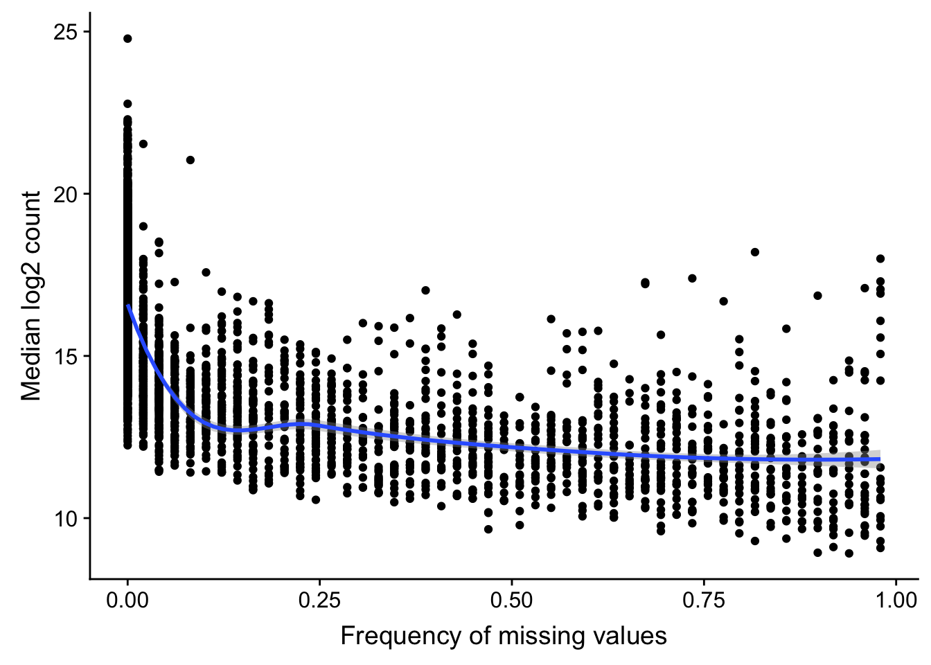
| Version | Author | Date |
|---|---|---|
| cc8c163 | Junyan Lu | 2020-02-27 |
Highly expressed proteins tend to have higher detection rate.
Remove proteins with more than 50% missing values
cut=0.5
protCLL_filt <- protCLL[rowSums(is.na(assay(protCLL)))/ncol(protCLL) < cut,]
Dimension of the filtered data
dim(protCLL_filt)[1] 3329 49Data normalization
Distribution of raw data
protTab <- sumToTiday(protCLL_filt, "uniprotID","patientID")
ggplot(protTab, aes(x=patientID, y=count)) + geom_boxplot() + scale_y_log10() +
  theme(axis.text.x = element_text(angle = 90, vjust = 0.5, hjust=1))
Warning: Removed 10891 rows containing non-finite values (stat_boxplot).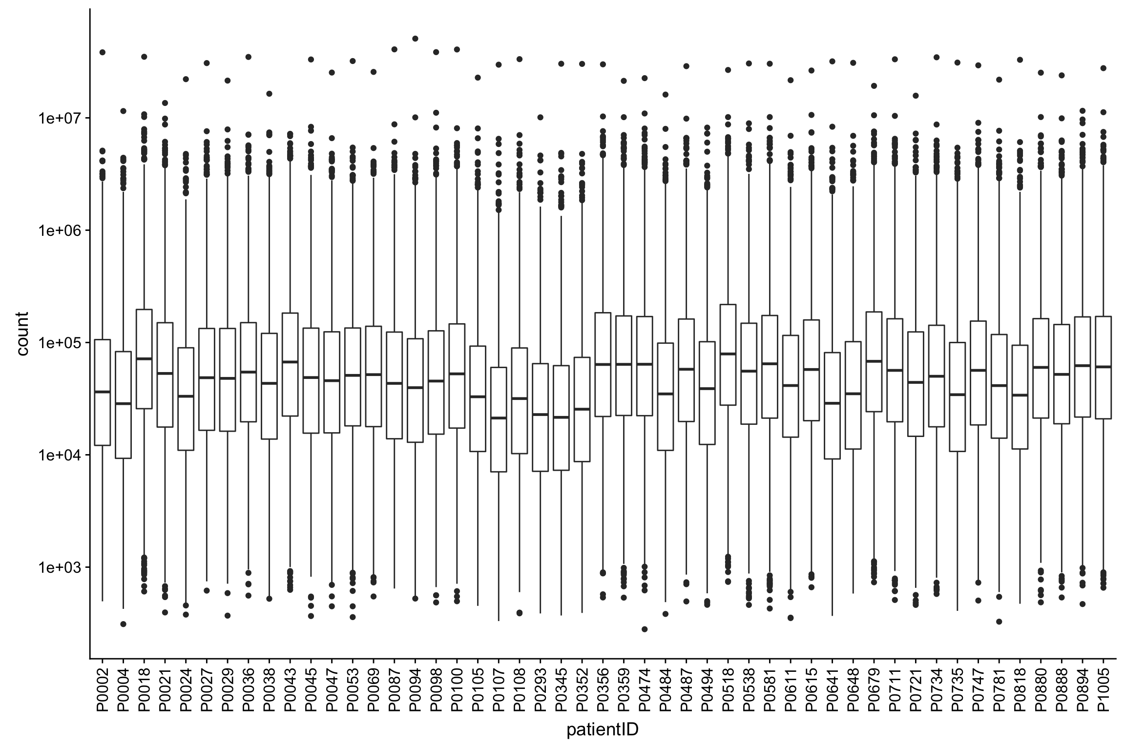
| Version | Author | Date |
|---|---|---|
| cc8c163 | Junyan Lu | 2020-02-27 |
Normalize data using vsn package
exprMat <- assay(protCLL_filt)
resVsn <- vsnMatrix(exprMat)
protCLL_norm <- protCLL_filt
assay(protCLL_norm) <- predict(resVsn, exprMat)
Boxplot of normalized counts
protTab <- sumToTiday(protCLL_norm, "uniprotID","patientID")
ggplot(protTab, aes(x=patientID, y=count)) + geom_boxplot() +
  theme(axis.text.x = element_text(angle = 90, vjust = 0.5, hjust=1))
Warning: Removed 10891 rows containing non-finite values (stat_boxplot).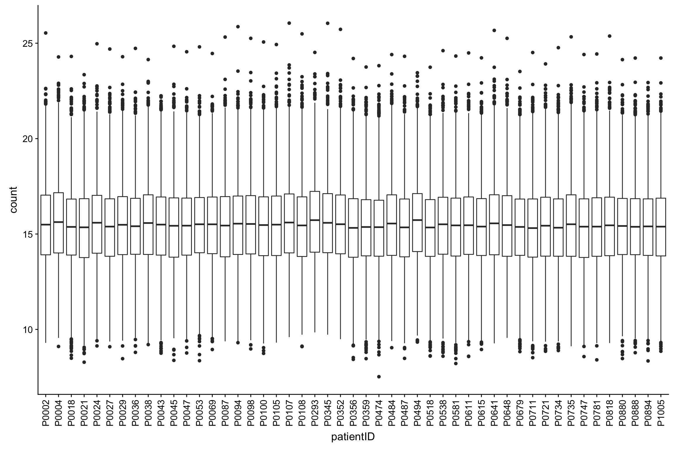
| Version | Author | Date |
|---|---|---|
| cc8c163 | Junyan Lu | 2020-02-27 |
Mean VS SD plot after normalization
vsn::meanSdPlot(resVsn)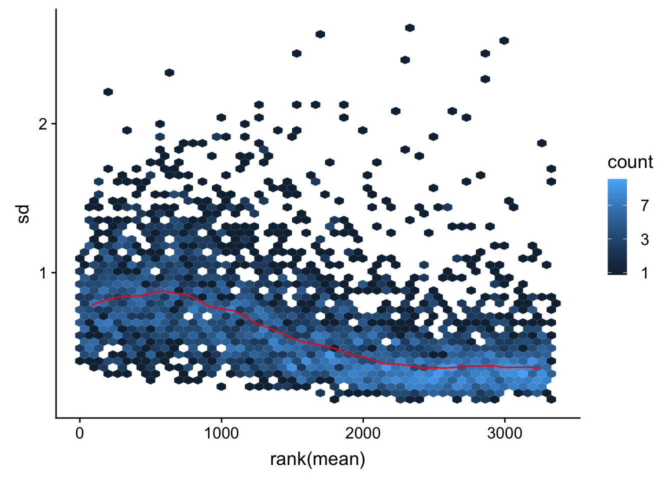
| Version | Author | Date |
|---|---|---|
| cc8c163 | Junyan Lu | 2020-02-27 |
Looks OK. Although lowly expressed proteins still have higher variance.
Impute missing values
For impute missing values, first I need to see whether the data is missing at random or not.
Check missing value pattern again (random or not?)
Missing value pattern after normalization and filtering
plot_missval(protCLL_norm)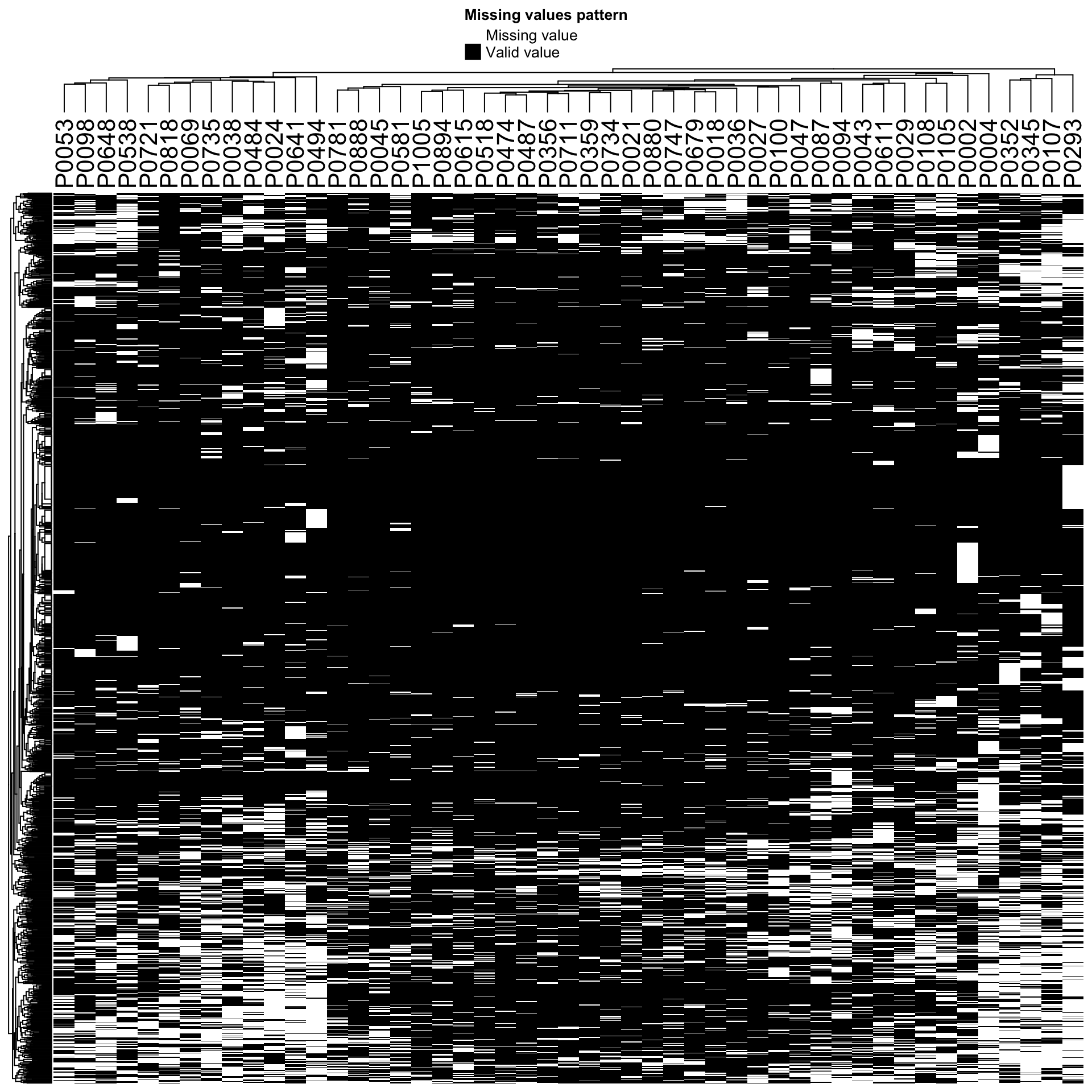
| Version | Author | Date |
|---|---|---|
| cc8c163 | Junyan Lu | 2020-02-27 |
Detection rate of proteins with and without missing values
plot_detect(protCLL_norm)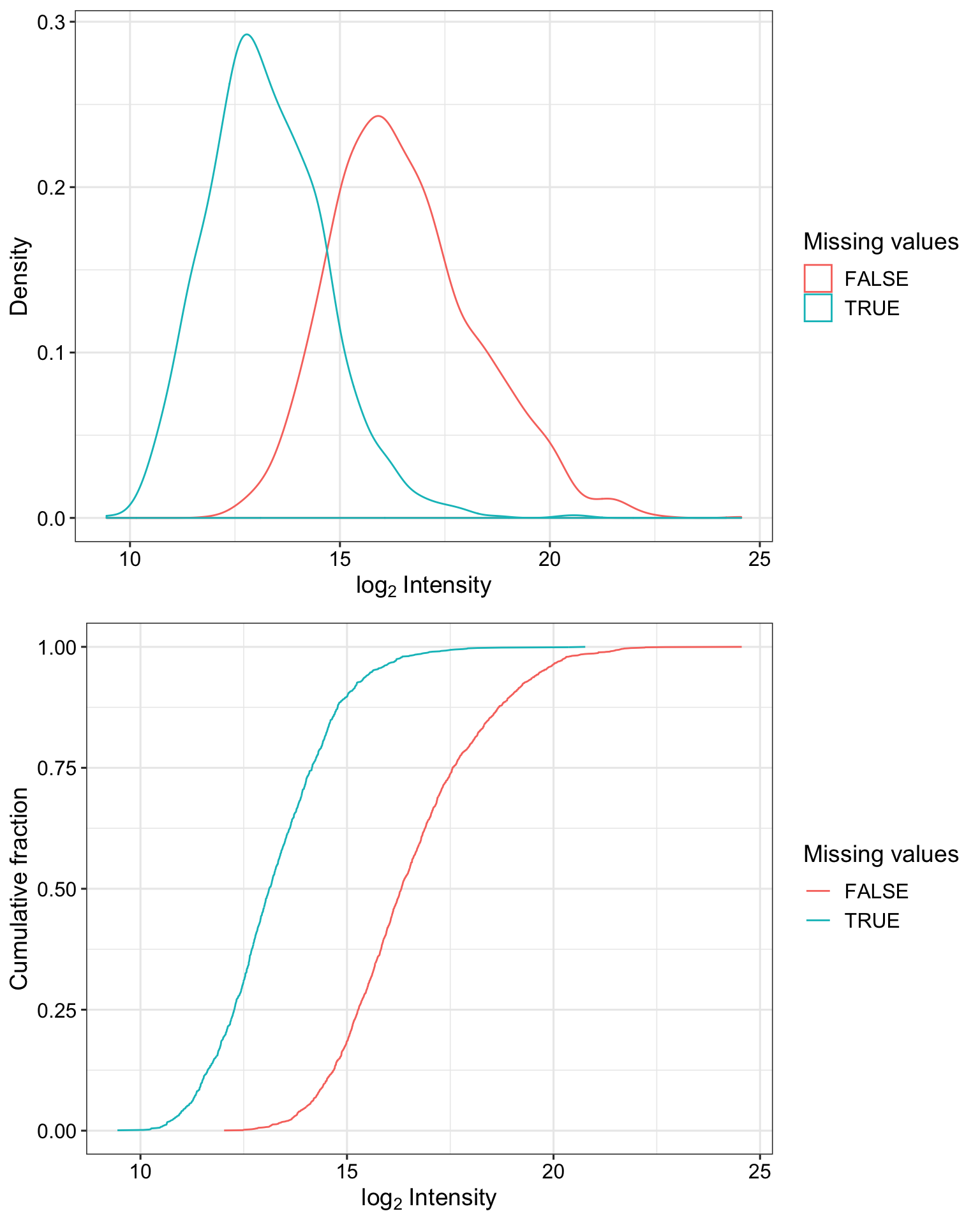
| Version | Author | Date |
|---|---|---|
| cc8c163 | Junyan Lu | 2020-02-27 |
Proteins with missing values have on average low intensities. Not missing at random.
Post-processing
Impute missing values
Impute missing values using quantile regression-based left-censored function (QRILC)
This is a method for imputing missing not at random data.
protCLL_imp <- impute(protCLL_norm, fun = "QRILC")Save objects
#add QRILC imputed data
assays(protCLL_norm)[["QRILC"]] <- assay(protCLL_imp)

protCLL_raw <- protCLL
protCLL <- protCLL_norm
#for other projects
save(protCLL, protCLL_raw, file = "../../var/proteomic_timsTOF_20200227.RData")

#for this project
save(protCLL, protCLL_raw, file = "../output/proteomic_timsTOF_20200227.RData")
sessionInfo()R version 3.6.0 (2019-04-26)
Platform: x86_64-apple-darwin15.6.0 (64-bit)
Running under: macOS Mojave 10.14.6
Matrix products: default
BLAS: /Library/Frameworks/R.framework/Versions/3.6/Resources/lib/libRblas.0.dylib
LAPACK: /Library/Frameworks/R.framework/Versions/3.6/Resources/lib/libRlapack.dylib
locale:
[1] en_US.UTF-8/en_US.UTF-8/en_US.UTF-8/C/en_US.UTF-8/en_US.UTF-8
attached base packages:
[1] stats4 parallel stats graphics grDevices utils datasets
[8] methods base
other attached packages:
[1] forcats_0.4.0 stringr_1.4.0
[3] dplyr_0.8.3 purrr_0.3.3
[5] readr_1.3.1 tidyr_1.0.0
[7] tibble_2.1.3 tidyverse_1.3.0
[9] SummarizedExperiment_1.14.0 DelayedArray_0.10.0
[11] BiocParallel_1.18.0 matrixStats_0.54.0
[13] GenomicRanges_1.36.0 GenomeInfoDb_1.20.0
[15] IRanges_2.18.1 S4Vectors_0.22.0
[17] biomaRt_2.40.0 DEP_1.6.1
[19] jyluMisc_0.1.5 vsn_3.52.0
[21] Biobase_2.44.0 BiocGenerics_0.30.0
[23] pheatmap_1.0.12 cowplot_0.9.4
[25] ggplot2_3.2.1 limma_3.40.2
loaded via a namespace (and not attached):
[1] utf8_1.1.4 shinydashboard_0.7.1 gmm_1.6-2
[4] tidyselect_0.2.5 RSQLite_2.1.1 AnnotationDbi_1.46.0
[7] htmlwidgets_1.3 grid_3.6.0 norm_1.0-9.5
[10] maxstat_0.7-25 munsell_0.5.0 codetools_0.2-16
[13] preprocessCore_1.46.0 DT_0.7 withr_2.1.2
[16] colorspace_1.4-1 knitr_1.23 rstudioapi_0.10
[19] ggsignif_0.5.0 mzID_1.22.0 labeling_0.3
[22] git2r_0.26.1 slam_0.1-45 GenomeInfoDbData_1.2.1
[25] KMsurv_0.1-5 bit64_0.9-7 rprojroot_1.3-2
[28] vctrs_0.2.0 generics_0.0.2 TH.data_1.0-10
[31] xfun_0.8 sets_1.0-18 R6_2.4.0
[34] doParallel_1.0.14 clue_0.3-57 bitops_1.0-6
[37] fgsea_1.10.0 assertthat_0.2.1 promises_1.0.1
[40] scales_1.0.0 multcomp_1.4-10 gtable_0.3.0
[43] affy_1.62.0 sandwich_2.5-1 workflowr_1.6.0
[46] rlang_0.4.1 zeallot_0.1.0 cmprsk_2.2-8
[49] mzR_2.18.1 GlobalOptions_0.1.0 splines_3.6.0
[52] lazyeval_0.2.2 impute_1.58.0 hexbin_1.27.3
[55] broom_0.5.2 modelr_0.1.5 BiocManager_1.30.4
[58] yaml_2.2.0 abind_1.4-5 backports_1.1.4
[61] httpuv_1.5.1 tools_3.6.0 relations_0.6-8
[64] ellipsis_0.2.0 affyio_1.54.0 gplots_3.0.1.1
[67] RColorBrewer_1.1-2 MSnbase_2.10.1 Rcpp_1.0.1
[70] plyr_1.8.4 progress_1.2.2 visNetwork_2.0.7
[73] zlibbioc_1.30.0 RCurl_1.95-4.12 prettyunits_1.0.2
[76] ggpubr_0.2.1 GetoptLong_0.1.7 zoo_1.8-6
[79] haven_2.2.0 cluster_2.1.0 exactRankTests_0.8-30
[82] fs_1.3.1 magrittr_1.5 data.table_1.12.2
[85] openxlsx_4.1.0.1 circlize_0.4.6 reprex_0.3.0
[88] survminer_0.4.4 pcaMethods_1.76.0 mvtnorm_1.0-11
[91] whisker_0.3-2 ProtGenerics_1.16.0 hms_0.5.2
[94] shinyjs_1.0 mime_0.7 evaluate_0.14
[97] xtable_1.8-4 XML_3.98-1.20 rio_0.5.16
[100] readxl_1.3.1 gridExtra_2.3 shape_1.4.4
[103] compiler_3.6.0 KernSmooth_2.23-15 ncdf4_1.16.1
[106] crayon_1.3.4 htmltools_0.3.6 later_0.8.0
[109] lubridate_1.7.4 DBI_1.0.0 dbplyr_1.4.2
[112] ComplexHeatmap_2.0.0 MASS_7.3-51.4 tmvtnorm_1.4-10
[115] Matrix_1.2-17 car_3.0-3 cli_1.1.0
[118] imputeLCMD_2.0 marray_1.62.0 gdata_2.18.0
[121] igraph_1.2.4.1 pkgconfig_2.0.2 km.ci_0.5-2
[124] foreign_0.8-71 piano_2.0.2 xml2_1.2.2
[127] MALDIquant_1.19.3 foreach_1.4.4 XVector_0.24.0
[130] drc_3.0-1 rvest_0.3.5 digest_0.6.19
[133] rmarkdown_1.13 cellranger_1.1.0 fastmatch_1.1-0
[136] survMisc_0.5.5 curl_3.3 shiny_1.3.2
[139] gtools_3.8.1 rjson_0.2.20 lifecycle_0.1.0
[142] nlme_3.1-140 jsonlite_1.6 carData_3.0-2
[145] fansi_0.4.0 pillar_1.4.2 lattice_0.20-38
[148] httr_1.4.1 plotrix_3.7-6 survival_2.44-1.1
[151] glue_1.3.1 zip_2.0.2 png_0.1-7
[154] iterators_1.0.10 bit_1.1-14 stringi_1.4.3
[157] blob_1.1.1 memoise_1.1.0 caTools_1.17.1.2