Quality control of the proteomic data from LUMOS machine
Junyan Lu
2020-02-27
Last updated: 2020-04-30
Checks: 6 1
Knit directory: Proteomics/analysis/
This reproducible R Markdown analysis was created with workflowr (version 1.6.0). The Checks tab describes the reproducibility checks that were applied when the results were created. The Past versions tab lists the development history.
The R Markdown file has unstaged changes. To know which version of the R Markdown file created these results, you’ll want to first commit it to the Git repo. If you’re still working on the analysis, you can ignore this warning. When you’re finished, you can run wflow_publish to commit the R Markdown file and build the HTML.
Great job! The global environment was empty. Objects defined in the global environment can affect the analysis in your R Markdown file in unknown ways. For reproduciblity it’s best to always run the code in an empty environment.
The command set.seed(20200227) was run prior to running the code in the R Markdown file. Setting a seed ensures that any results that rely on randomness, e.g. subsampling or permutations, are reproducible.
Great job! Recording the operating system, R version, and package versions is critical for reproducibility.
Nice! There were no cached chunks for this analysis, so you can be confident that you successfully produced the results during this run.
Great job! Using relative paths to the files within your workflowr project makes it easier to run your code on other machines.
Great! You are using Git for version control. Tracking code development and connecting the code version to the results is critical for reproducibility. The version displayed above was the version of the Git repository at the time these results were generated.
Note that you need to be careful to ensure that all relevant files for the analysis have been committed to Git prior to generating the results (you can use wflow_publish or wflow_git_commit). workflowr only checks the R Markdown file, but you know if there are other scripts or data files that it depends on. Below is the status of the Git repository when the results were generated:
Ignored files:
    Ignored:    .DS_Store
    Ignored:    .Rhistory
    Ignored:    .Rproj.user/
    Ignored:    analysis/.DS_Store
    Ignored:    analysis/.Rhistory
    Ignored:    analysis/analysisTrisomy19_cache/
    Ignored:    analysis/correlateGenomic_PC12adjusted_cache/
    Ignored:    analysis/correlateGenomic_cache/
    Ignored:    analysis/correlateGenomic_noBlock_MCLL_cache/
    Ignored:    analysis/correlateGenomic_noBlock_UCLL_cache/
    Ignored:    analysis/correlateGenomic_noBlock_cache/
    Ignored:    analysis/figure/
    Ignored:    code/.Rhistory
    Ignored:    data/.DS_Store
    Ignored:    output/.DS_Store

Untracked files:
    Untracked:  analysis/analysisSplicing.Rmd
    Untracked:  analysis/analysisTrisomy19.Rmd
    Untracked:  analysis/annotateCNV.Rmd
    Untracked:  analysis/correlateGenomic_PC12adjusted.Rmd
    Untracked:  analysis/correlateGenomic_noBlock.Rmd
    Untracked:  analysis/correlateGenomic_noBlock_MCLL.Rmd
    Untracked:  analysis/correlateGenomic_noBlock_UCLL.Rmd
    Untracked:  analysis/default.css
    Untracked:  analysis/peptideValidate.Rmd
    Untracked:  analysis/plotExpressionCNV.Rmd
    Untracked:  analysis/processPeptides_LUMOS.Rmd
    Untracked:  analysis/style.css
    Untracked:  code/utils.R
    Untracked:  data/190909_CLL_prot_abund_med_norm.tsv
    Untracked:  data/190909_CLL_prot_abund_no_norm.tsv
    Untracked:  data/20190423_Proteom_submitted_samples_bereinigt.xlsx
    Untracked:  data/20191025_Proteom_submitted_samples_final.xlsx
    Untracked:  data/LUMOS/
    Untracked:  data/LUMOS_peptides/
    Untracked:  data/LUMOS_protAnnotation.csv
    Untracked:  data/LUMOS_protAnnotation_fix.csv
    Untracked:  data/SampleAnnotation_cleaned.xlsx
    Untracked:  data/facTab_IC50atLeast3New.RData
    Untracked:  data/gmts/
    Untracked:  data/mapEnsemble.txt
    Untracked:  data/mapSymbol.txt
    Untracked:  data/pyprophet_export_aligned.csv
    Untracked:  data/timsTOF_protAnnotation.csv
    Untracked:  output/LUMOS_processed.RData
    Untracked:  output/dxdCLL.RData
    Untracked:  output/pepCLL_lumos.RData
    Untracked:  output/pepTab_lumos.RData
    Untracked:  output/proteomic_LUMOS_20200227.RData
    Untracked:  output/proteomic_LUMOS_20200320.RData
    Untracked:  output/proteomic_LUMOS_20200430.RData
    Untracked:  output/proteomic_timsTOF_20200227.RData
    Untracked:  output/splicingResults.RData
    Untracked:  output/timsTOF_processed.RData

Unstaged changes:
    Modified:   analysis/_site.yml
    Modified:   analysis/analysisSF3B1.Rmd
    Modified:   analysis/compareProteomicsRNAseq.Rmd
    Modified:   analysis/correlateGenomic.Rmd
    Deleted:    analysis/correlateGenomic_removePC.Rmd
    Modified:   analysis/correlateMIR.Rmd
    Modified:   analysis/correlateMethylationCluster.Rmd
    Modified:   analysis/index.Rmd
    Modified:   analysis/predictOutcome.Rmd
    Modified:   analysis/processProteomics_LUMOS.Rmd
    Modified:   analysis/qualityControl_LUMOS.Rmd
Note that any generated files, e.g. HTML, png, CSS, etc., are not included in this status report because it is ok for generated content to have uncommitted changes.
These are the previous versions of the R Markdown and HTML files. If you’ve configured a remote Git repository (see ?wflow_git_remote), click on the hyperlinks in the table below to view them.
| File | Version | Author | Date | Message |
|---|---|---|---|---|
| html | 8ba49d7 | Junyan Lu | 2020-03-17 | Build site. |
| Rmd | 0f1820c | Junyan Lu | 2020-03-17 | update quality control |
| html | b8e0823 | Junyan Lu | 2020-03-10 | Build site. |
| Rmd | c7747b2 | Junyan Lu | 2020-03-10 | update analysses |
| html | c7747b2 | Junyan Lu | 2020-03-10 | update analysses |
| html | 46534c2 | Junyan Lu | 2020-02-27 | Build site. |
| Rmd | 2b8852e | Junyan Lu | 2020-02-27 | wflow_publish(list.files(“./”, pattern = “Rmd”)) |
Test association with RNA expression
Dimension of the inputed data
dim(protCLL)[1] 4316 49Process both datasets
colnames(dds) <- dds$PatID
dds <- estimateSizeFactors(dds)
sampleOverlap <- intersect(colnames(protCLL), colnames(dds))
geneOverlap <- intersect(rowData(protCLL)$ensembl_gene_id, rownames(dds))
ddsSub <- dds[geneOverlap, sampleOverlap]
protSub <- protCLL[match(geneOverlap, rowData(protCLL)$ensembl_gene_id), sampleOverlap]

#how many gene don't have RNA expression at all?
noExp <- rowSums(counts(ddsSub)) == 0
sum(noExp)
[1] 5#remove those genes in both datasets
ddsSub <- ddsSub[!noExp,]
protSub <- protSub[!noExp,]
#remove proteins with duplicated identifiers
protSub <- protSub[!duplicated(rowData(protSub)$name)]
geneOverlap <- intersect(rowData(protSub)$ensembl_gene_id, rownames(ddsSub))
ddsSub.vst <- varianceStabilizingTransformation(ddsSub)Calculate correlations between protein abundance and RNA expression
rnaMat <- assay(ddsSub.vst)
proMat.raw <- assays(protSub)[["count"]]
proMat.qrilc <- assays(protSub)[["QRILC"]]
rownames(proMat.qrilc) <- rowData(protSub)$ensembl_gene_id
rownames(proMat.raw) <- rowData(protSub)$ensembl_gene_id

corTab <- lapply(geneOverlap, function(n) {
  rna <- rnaMat[n,]
  pro.q <- proMat.qrilc[n,]
  pro.raw <- proMat.raw[n,]
  res.q <- cor.test(rna, pro.q)
  res.raw <- cor.test(rna, pro.raw, use = "pairwise.complete.obs")
  tibble(id = n, impute=c("No Imputation","QRILC"),
         p = c(res.raw$p.value, res.q$p.value),
         coef = c(res.raw$estimate, res.q$estimate))
}) %>% bind_rows() %>%
  arrange(desc(coef)) %>% mutate(p.adj = p.adjust(p, method = "BH"),
                                 symbol = rowData(dds[id,])$symbol)
Plot the distribution of correlation coefficient
ggplot(corTab, aes(x=coef, fill = impute)) + geom_histogram(position = "identity", col = "grey50", alpha =0.3, bins =100) +
  geom_vline(xintercept = 0, col = "red", linetype = "dashed")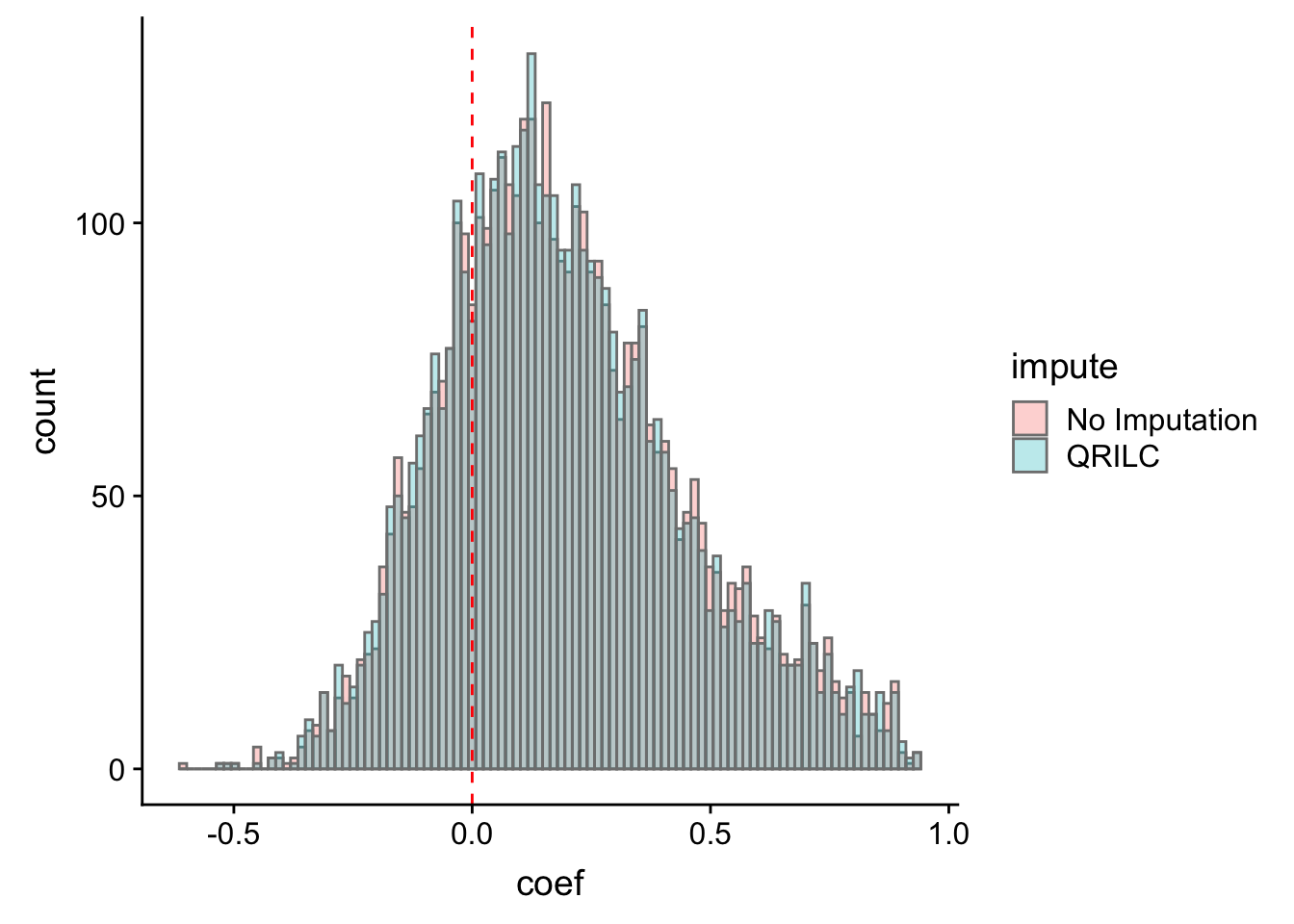
| Version | Author | Date |
|---|---|---|
| 46534c2 | Junyan Lu | 2020-02-27 |
Most of the correlations are positive, which is reasonable.
Number of significant positive and negative correlations (10% FDR)
sigTab <- corTab %>% filter(p.adj < 0.1) %>% mutate(direction = ifelse(coef > 0, "positive", "negative")) %>%
  group_by(impute, direction) %>% summarise(number = length(id)) %>% ungroup() %>%
  mutate(ratio = format(number/length(geneOverlap), digits = 2)) %>% arrange(number)
DT::datatable(sigTab)
Number of significant correlations VS FDR cut-off
plotTab <- lapply(seq(0,0.1, length.out = 100), function(fdr) {
  filTab <- dplyr::filter(corTab, p.adj < fdr, coef > 0) %>%
    group_by(impute) %>% summarise(n = length(id)) %>% mutate(fdr = fdr)
}) %>% bind_rows()

ggplot(plotTab, aes(x=fdr, y = n, col = impute))+ geom_line() +
  ylab("Number of significant correlations") +
  xlab("FDR cut-off")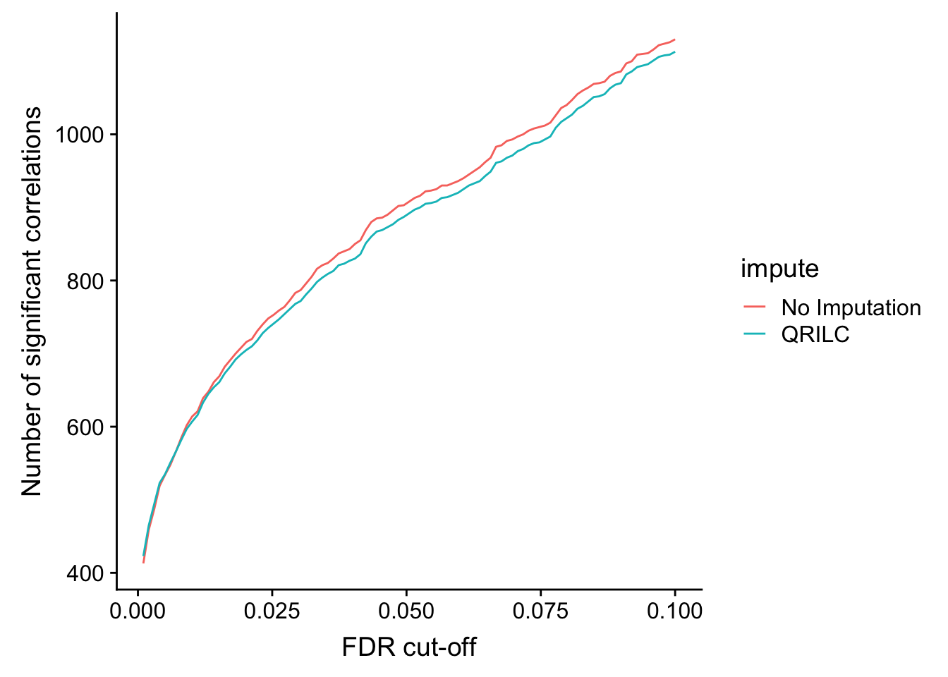
| Version | Author | Date |
|---|---|---|
| 46534c2 | Junyan Lu | 2020-02-27 |
List of proteins that significantly correlated with RNA expression (10 %FDR, no imputation)
sigTab <- filter(corTab, p.adj < 0.1, impute == "No Imputation") %>% mutate_if(is.numeric, format, digits=2)
DT::datatable(sigTab)
List of proteins that significantly correlated with RNA expression (10 %FDR, QRILC imputed)
sigTab <- filter(corTab, p.adj < 0.1, impute == "QRILC") %>% mutate_if(is.numeric, format, digits=2)
DT::datatable(sigTab)
Correlation plot of top 9 most correlated protein-rna pairs
plotList <- lapply(sigTab$id[1:9], function(n) {
  plotTab <- tibble(pro = proMat.qrilc[n,], gene = rnaMat[n,])
  symbol <- filter(sigTab, id == n)$symbol
  ggplot(plotTab, aes(x=pro, y=gene)) + geom_point() + geom_smooth(method = "lm") +
    ggtitle(symbol) + ylab("RNA expression") + xlab("Protein abundance")
})

cowplot::plot_grid(plotlist = plotList, ncol =3)
`geom_smooth()` using formula 'y ~ x'
`geom_smooth()` using formula 'y ~ x'
`geom_smooth()` using formula 'y ~ x'
`geom_smooth()` using formula 'y ~ x'
`geom_smooth()` using formula 'y ~ x'
`geom_smooth()` using formula 'y ~ x'
`geom_smooth()` using formula 'y ~ x'
`geom_smooth()` using formula 'y ~ x'
`geom_smooth()` using formula 'y ~ x'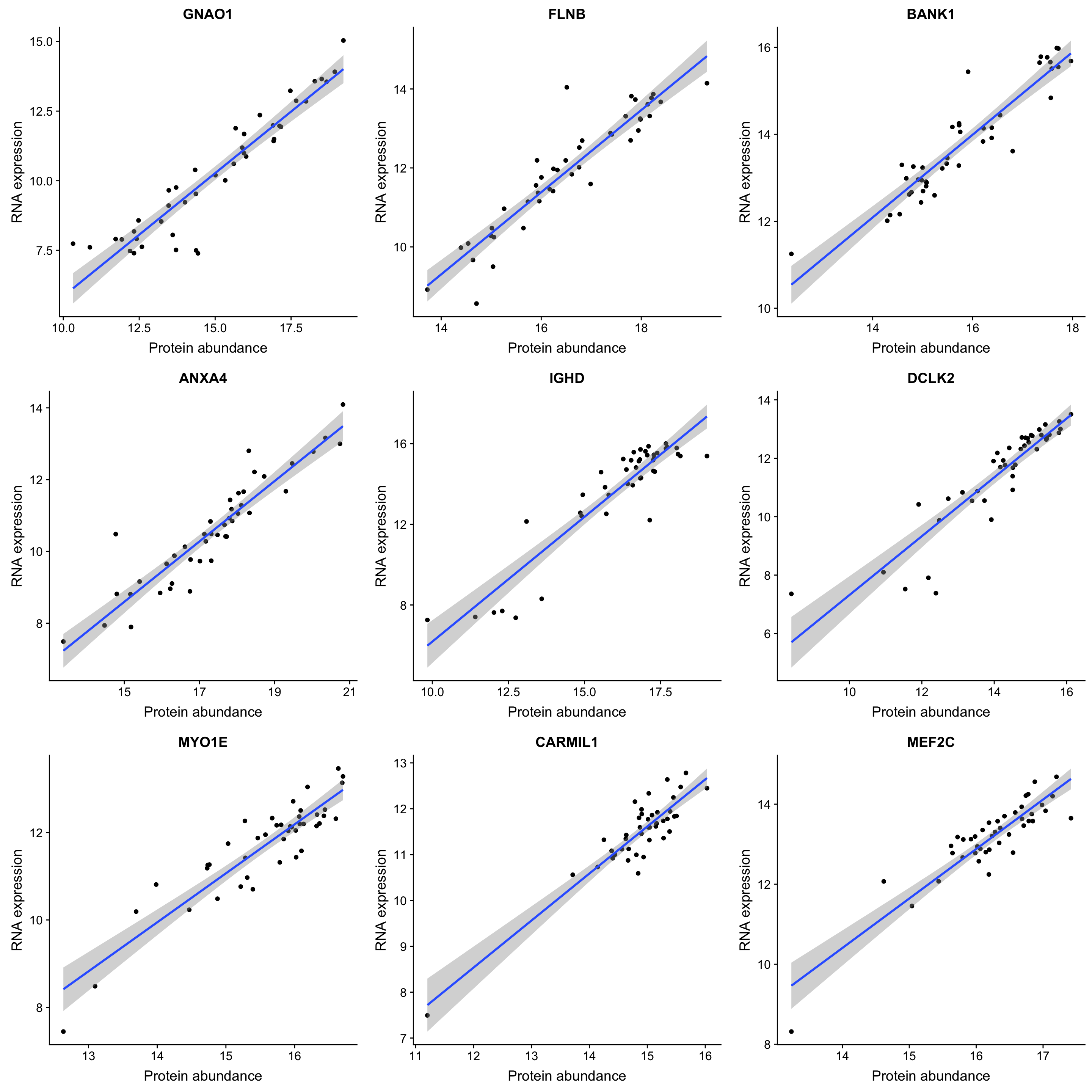
| Version | Author | Date |
|---|---|---|
| 46534c2 | Junyan Lu | 2020-02-27 |
Scater plot of protein pairs show significant correlations
idList <- filter(corTab, p.adj <= 0.1, coef > 0, impute == "No Imputation")$id
protTab.raw <- proMat.raw[idList, ] %>% data.frame() %>% rownames_to_column("id") %>%
  gather(key = "patID", value = "protein", -id)
rnaTab.raw <- rnaMat[idList, ] %>% data.frame() %>% rownames_to_column("id") %>%
  gather(key = "patID", value = "rna", -id)
plotTab <- left_join(protTab.raw, rnaTab.raw, by = c("patID","id"))
ggplot(plotTab, aes(x=rna, y = protein)) + geom_point(aes(col = patID), alpha =0.5) + geom_smooth(method = "lm")
`geom_smooth()` using formula 'y ~ x'Warning: Removed 1258 rows containing non-finite values (stat_smooth).Warning: Removed 1258 rows containing missing values (geom_point).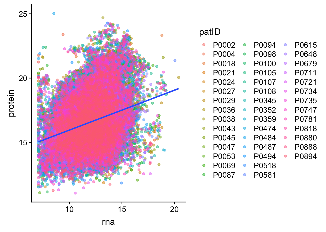
| Version | Author | Date |
|---|---|---|
| b8e0823 | Junyan Lu | 2020-03-10 |
Assocation with technical factors
Are thechnical variables confounded with major genomic variabes?
# A tibble: 3 x 4
  genomic     technical      pval  p.adj
  <chr>       <chr>         <dbl>  <dbl>
1 trisomy12   proteinConc 0.00185 0.0778
2 IGHV.status processDate 0.0277  0.581
3 del13q      operator    0.0494  0.581
Trisomy12 has some impact on total protein concentration, but not very strong
Trisomy12 versus protein concentration
plotTab <- tibble(gene = geneTab$trisomy12, proteinConc = techTab$proteinConc)
ggplot(plotTab, aes(x=gene, y = proteinConc)) + geom_boxplot() + geom_point()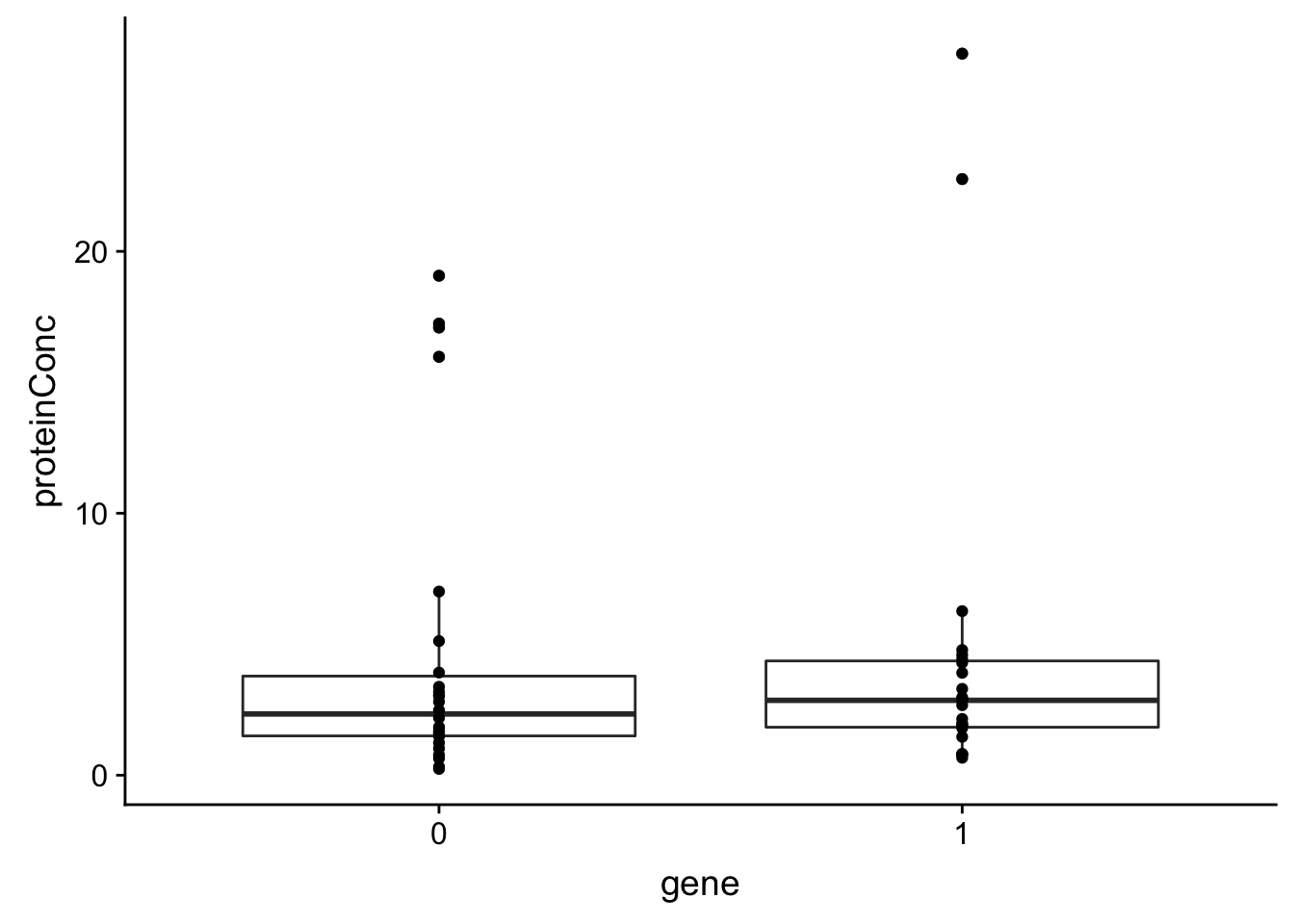
| Version | Author | Date |
|---|---|---|
| b8e0823 | Junyan Lu | 2020-03-10 |
There’s a small trend that trisomy12 samples tend to have higher protein concentration.
Association between technical variables and priciple components of protein expression
plotMat <- assays(protCLL)[["QRILC"]]
pcRes <- prcomp(t(plotMat), center =TRUE, scale. = FALSE)$x

testRes <- lapply(colnames(pcRes), function(pc) {
  lapply(colnames(techTab), function(tech) {
    pcVar <- pcRes[,pc]
    techVar <- techTab[[tech]]
    res <- summary(aov(pcVar ~ techVar))
    p <- res[[1]][1,4]
    tibble(component = pc, technical = tech, pval = p)
  }) %>% bind_rows()
}) %>% bind_rows() %>% mutate(p.adj = p.adjust(pval, method = "BH")) %>%
  arrange(pval)
filter(testRes, p.adj < 0.1)
# A tibble: 1 x 4
component technical pval p.adj
<chr> <chr> <dbl> <dbl>
1 PC26 proteinConc 0.0000741 0.0218There are some principle components correlated with technical variables. But the PCs are not top PCs, suggesting the know technical factor do not have impact on the major trends of the dataset.
Associations between technical variables and individual protein expressions
Association test
techTab <- colData(protCLL)[,c("operator", "viability","batch","processDate","proteinConc","freeThawCycle")] %>%
  data.frame() %>%rownames_to_column("patID") %>% as_tibble() %>% mutate(processDate = as.character(processDate)) %>%
  mutate_if(is.character, as.factor)%>% mutate_at(vars(-patID), as.numeric)
testTab <- assays(protCLL)[["QRILC"]] %>% data.frame() %>%
  rownames_to_column("id") %>% mutate(name = rowData(protCLL)[id,]$hgnc_symbol) %>%
  gather(key = "patID", value = "expr", -id, -name) %>%
  left_join(techTab, by ="patID") %>% gather(key = technical, value = value, -id, -name, -patID, -expr)
Warning: Column `patID` joining character vector and factor, coercing into
character vectortestRes <- filter(testTab, !is.na(value)) %>%
group_by(name, technical) %>% nest() %>%
mutate(m = map(data, ~lm(expr~value,.))) %>%
mutate(res = map(m, broom::tidy)) %>%
unnest(res) %>% filter(term=="value") %>%
ungroup() %>%
mutate(p.adj = p.adjust(p.value, method = "BH"))
sumTab <- filter(testRes, p.adj < 0.1) %>% group_by(technical) %>% summarise(n=length(name))
ggplot(sumTab, aes(x=technical, y = n)) + geom_bar(stat = "identity") + coord_flip() +
xlab("") + ylab("Number of significantly associated proteins")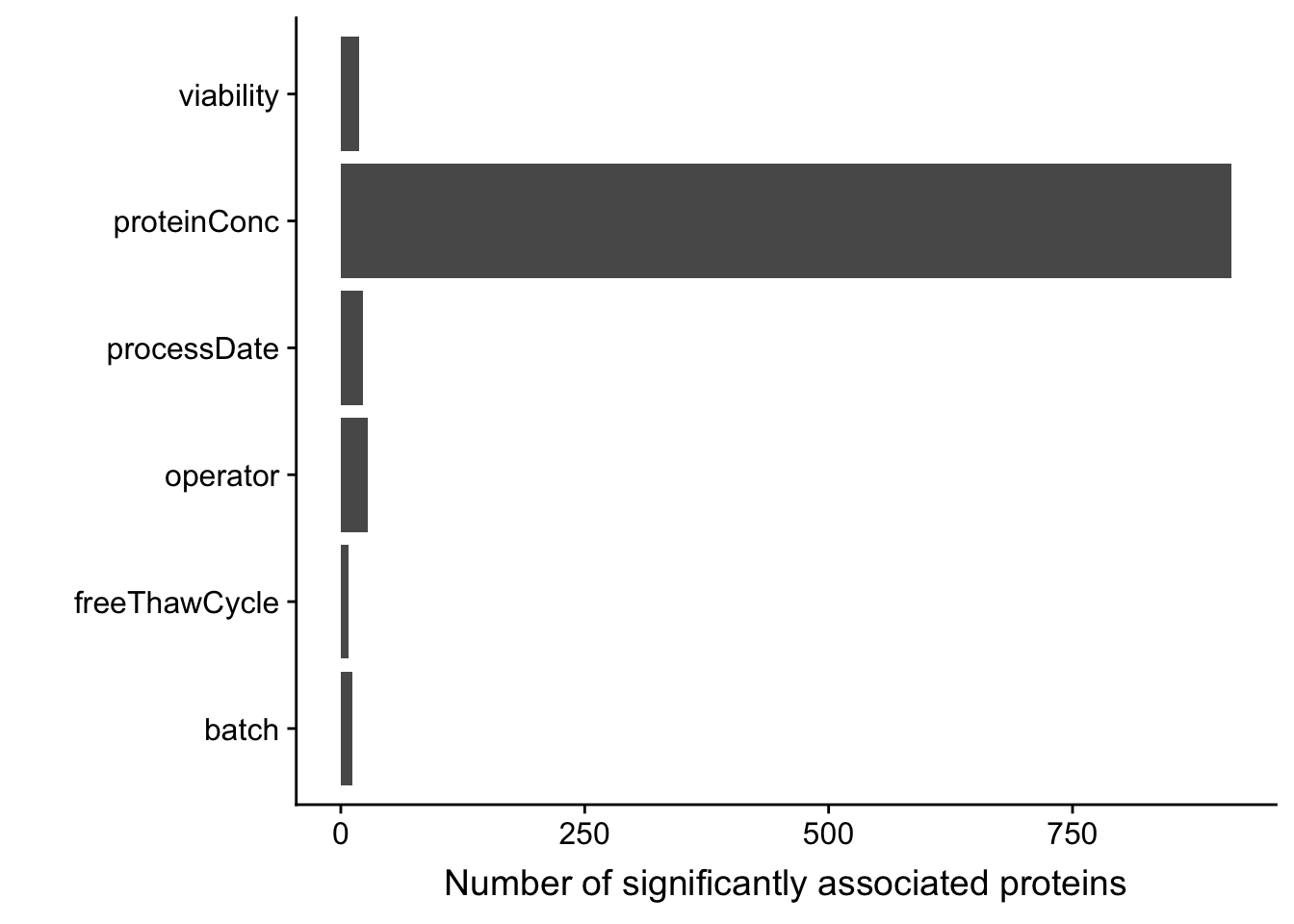
There are more than 750 proteins whose abundance may be significantly affected by overall protein concentration.
Assocation P value histogram for each technical factor
ggplot(testRes, aes(x=p.value)) + geom_histogram() + facet_wrap(~technical) + xlim(0,1)`stat_bin()` using `bins = 30`. Pick better value with `binwidth`.Warning: Removed 12 rows containing missing values (geom_bar).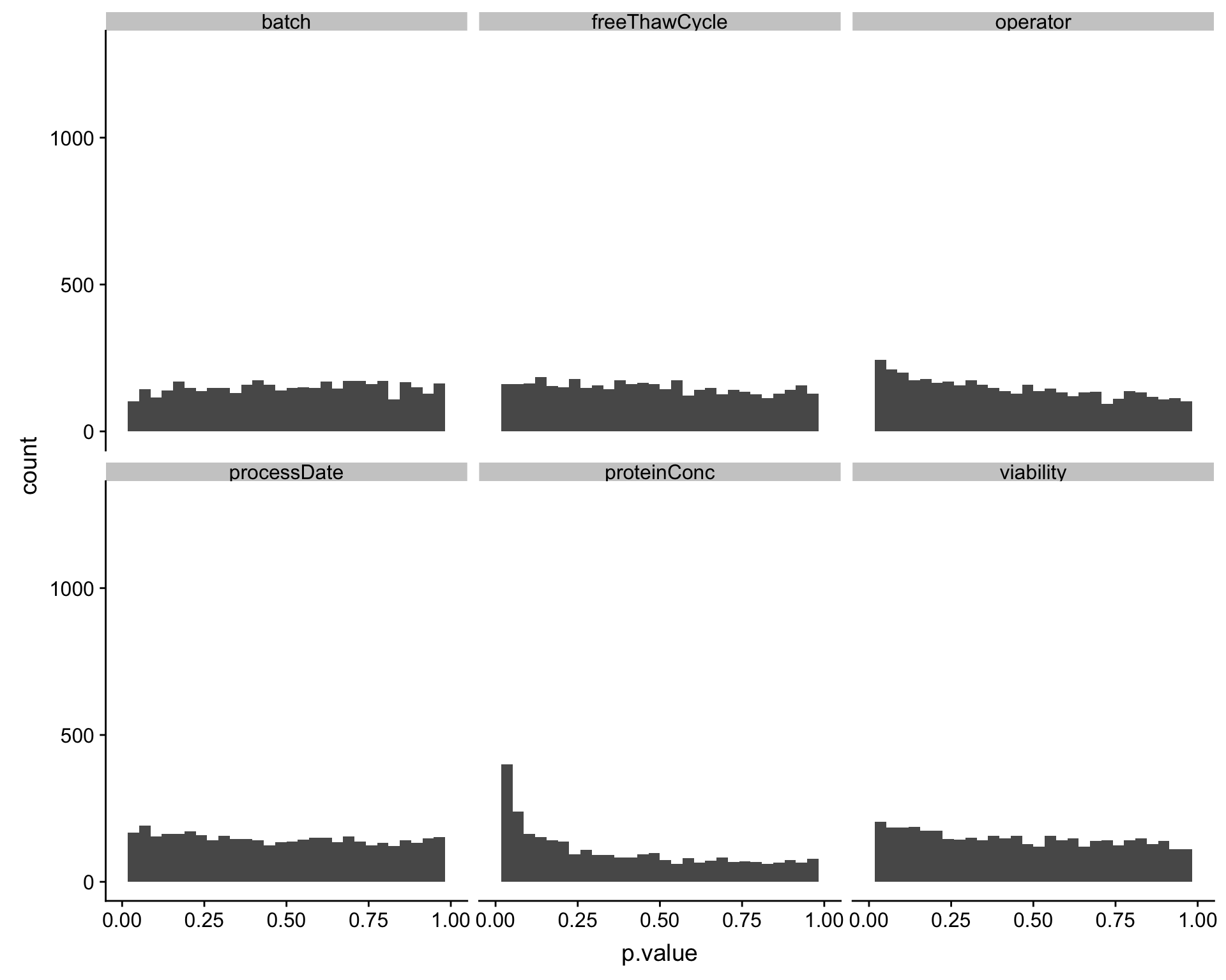
| Version | Author | Date |
|---|---|---|
| b8e0823 | Junyan Lu | 2020-03-10 |
Also based on the p-value histogram, only overall protein concentration may have potential impact on protein abundance detection.
List of proteins that show significant correlation with total protein concentration (10% FDR)
filter(testRes, technical == "proteinConc") %>% select(name, p.value, p.adj, estimate) %>%
  arrange(p.value) %>% filter(p.adj <= 0.1) %>%
  mutate_if(is.numeric, formatC, digits=2, format="e") %>%
  DT::datatable()
Will the correlation with RNA expression improve if we adjust for total protein concentration?
proteinConc <- techTab[match(colnames(proMat.qrilc), techTab$patID),]$proteinConc
corTab <- lapply(geneOverlap, function(n) {
  rna <- rnaMat[n,]
  pro.q <- proMat.qrilc[n,]
  p.single <- anova(lm(rna ~ pro.q))$`Pr(>F)`[1]
  p.multi <- car::Anova(lm(rna ~ pro.q + proteinConc))$`Pr(>F)`[1]
  tibble(name = n, corrected = c("no","yes"),
         p = c(p.single, p.multi))
}) %>% bind_rows() %>% mutate(p.adj = p.adjust(p, method = "BH")) %>% arrange(p)
Number of significant correlations VS FDR cut-off
plotTab <- lapply(seq(0,0.1, length.out = 100), function(fdr) {
  filTab <- dplyr::filter(corTab, p.adj < fdr) %>%
    group_by(corrected) %>% summarise(n = length(name)) %>% mutate(fdr = fdr)
}) %>% bind_rows()

ggplot(plotTab, aes(x=fdr, y = n, col = corrected))+ geom_line() +
  ylab("Number of significant correlations") +
  xlab("FDR cut-off")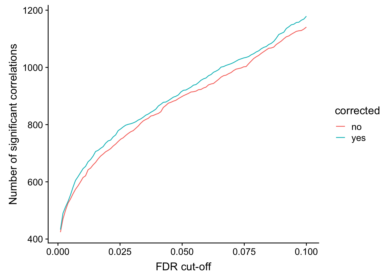
Seems to improve the correlation a little, but not much. We can include this factor in association test later.
List of proteins that show significant correlation with viability (10% FDR)
filter(testRes, technical == "viability") %>% select(name, p.value, p.adj, estimate) %>%
  arrange(p.value) %>% filter(p.adj <= 0.1) %>%
  mutate_if(is.numeric, formatC, digits=2, format="e") %>%
  DT::datatable()
Check data structure
Hierarchical clustering
plotMat <- assays(protCLL)[["QRILC"]]

colAnno <- colData(protCLL)[,c("gender","IGHV.status","trisomy12")] %>%
  data.frame()

plotMat <- jyluMisc::mscale(plotMat, censor = 6)
pheatmap(plotMat, scale = "none", annotation_col = colAnno, clustering_method = "ward.D2",
         show_rownames = FALSE, color = colorRampPalette(c("navy","white","firebrick"))(100),
         breaks = seq(-6,6, length.out = 101))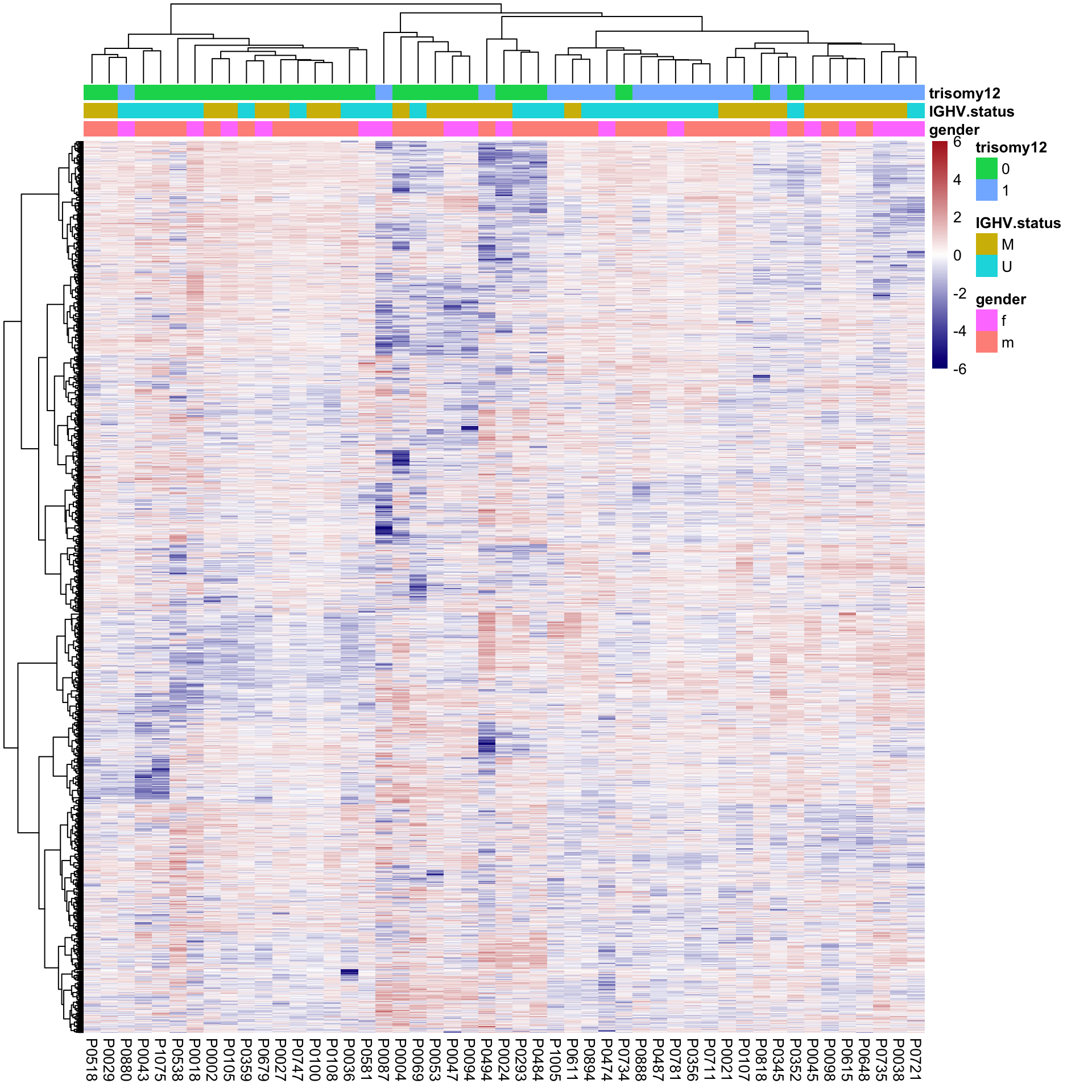
Some separation can be observed for trisomy12
PCA
pcOut <- prcomp(t(plotMat), center =TRUE, scale. = FALSE)
pcRes <- pcOut$x
eigs <- pcOut$sdev^2
varExp <- structure(eigs/sum(eigs),names = colnames(pcRes))

plotTab <- pcRes[,1:2] %>% data.frame() %>% cbind(colAnno[rownames(.),]) %>%
  rownames_to_column("patID") %>% as_tibble()

ggplot(plotTab, aes(x=PC1, y=PC2, col = IGHV.status, shape = trisomy12)) + geom_point(size=4) +
  xlab(sprintf("PC1 (%1.2f%%)",varExp[["PC1"]]*100)) +
  ylab(sprintf("PC2 (%1.2f%%)",varExp[["PC2"]]*100))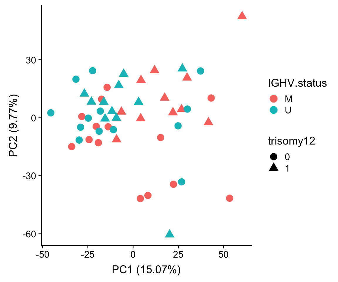
No strong separation can be observed.
Correlation PCs with trisomy12 and IGHV status
corTab <- lapply(colnames(pcRes),  function(pc) {
  ighvCor <- t.test(pcRes[,pc] ~ colAnno$IGHV.status)
  tri12Cor <- t.test(pcRes[,pc] ~ colAnno$trisomy12)
  tibble(PC = pc,
         feature=c("IGHV", "trisomy12"),
         p = c(ighvCor$p.value, tri12Cor$p.value))
}) %>% bind_rows() %>% mutate(p.adj = p.adjust(p, method = "BH")) %>%
  filter(p <= 0.05) %>% arrange(p)
corTab
# A tibble: 4 x 4
PC feature p p.adj
<chr> <chr> <dbl> <dbl>
1 PC3 trisomy12 1.72e-10 0.0000000168
2 PC4 IGHV 6.50e- 6 0.000319
3 PC2 trisomy12 1.83e- 2 0.598
4 PC1 IGHV 4.53e- 2 0.998 PCA plot using PC3 and PC4
plotTab <- pcRes[,1:10] %>% data.frame() %>% cbind(colAnno[rownames(.),]) %>%
  rownames_to_column("patID") %>% as_tibble()

ggplot(plotTab, aes(x=PC3, y=PC4, col = IGHV.status, shape = trisomy12, label = patID)) + geom_point() + ggrepel::geom_text_repel() +
  xlab(sprintf("PC3 (%1.2f%%)",varExp[["PC3"]]*100)) +
  ylab(sprintf("PC4 (%1.2f%%)",varExp[["PC4"]]*100))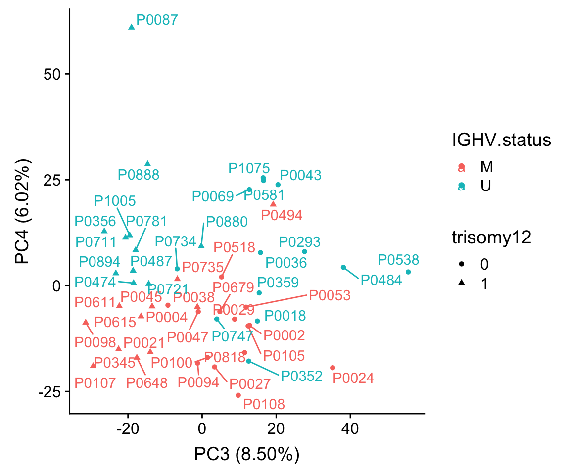
Using PC3 and PC4 better seperates IGHV and trisomy12.
Biological annotation of PC1 and PC2
Annotate PC1
Correlation test
Assocation test
proMat <- assays(protCLL)[["QRILC"]]
pc <- pcRes[,1][colnames(proMat)]
designMat <- model.matrix(~1+pc)
fit <- lmFit(proMat,  designMat)
fit2 <- eBayes(fit)
corRes.pc1 <- topTable(fit2, number ="all", adjust.method = "BH", coef = "pc") %>% rownames_to_column("id") %>%
    mutate(symbol = rowData(protCLL[id,])$hgnc_symbol)
Number of significant associations (10% FDR)
hist(corRes.pc1$P.Value,breaks=100)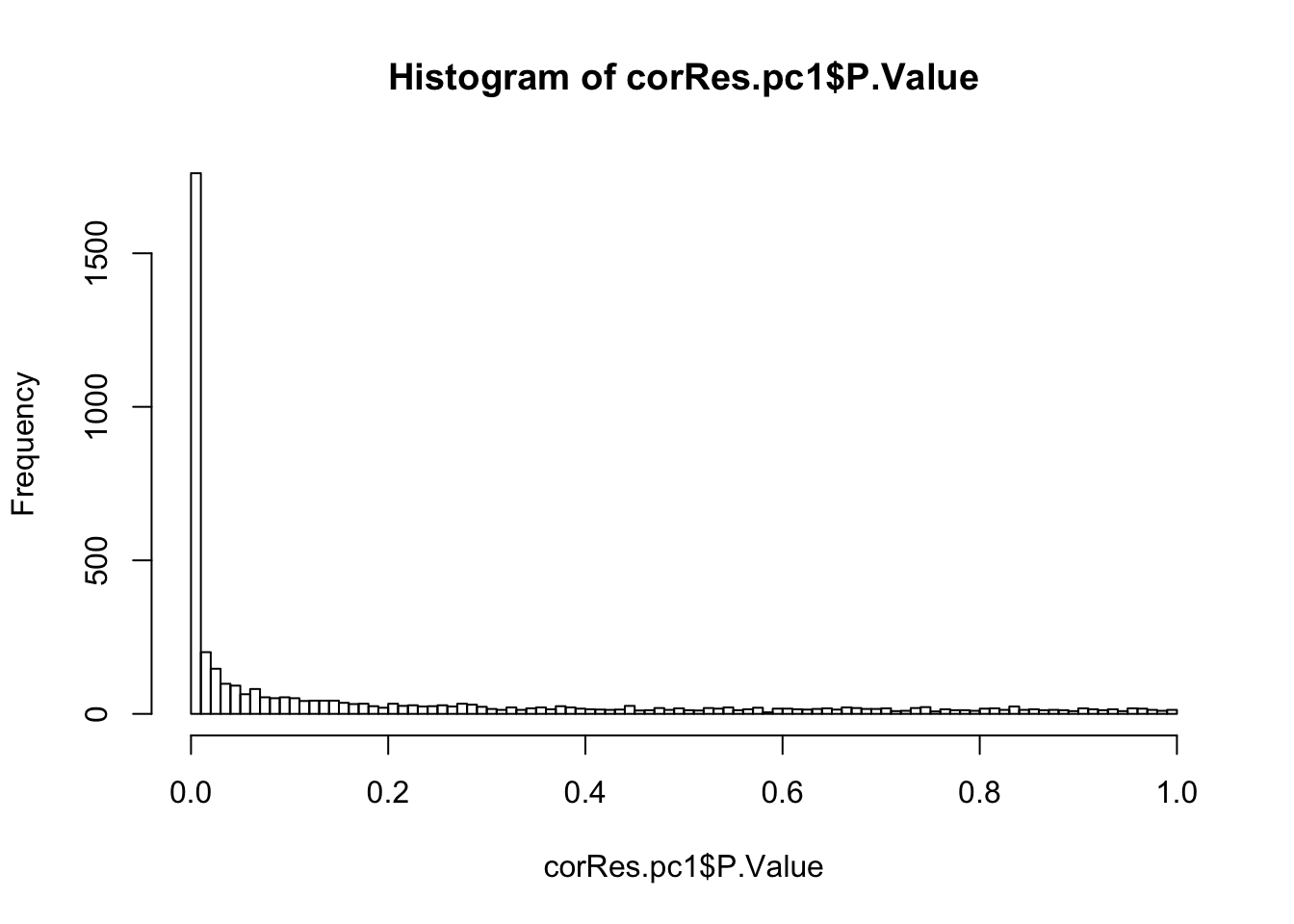
Table of significant associations (5% FDR)
resTab.sig <- filter(corRes.pc1, adj.P.Val < 0.05) %>%
  select(symbol, id,logFC, P.Value, adj.P.Val) %>%
  arrange(P.Value)
resTab.sig %>% mutate_if(is.numeric, formatC, digits=2, format= "e") %>%
  DT::datatable()
Heatmap of associated genes
colAnno <- tibble(patID = colnames(proMat), PC1 = pcRes[colnames(proMat),1]) %>%
  arrange(PC1) %>% data.frame() %>% column_to_rownames("patID")

plotMat <- proMat[resTab.sig$id[1:100],rownames(colAnno)]
plotMat <- jyluMisc::mscale(plotMat, censor = 6)

pheatmap(plotMat, scale = "none", annotation_col = colAnno, clustering_method = "ward.D2",
         cluster_cols = FALSE,
         labels_row = resTab.sig$symbol[1:100], color = colorRampPalette(c("navy","white","firebrick"))(100),
         breaks = seq(-6,6, length.out = 101))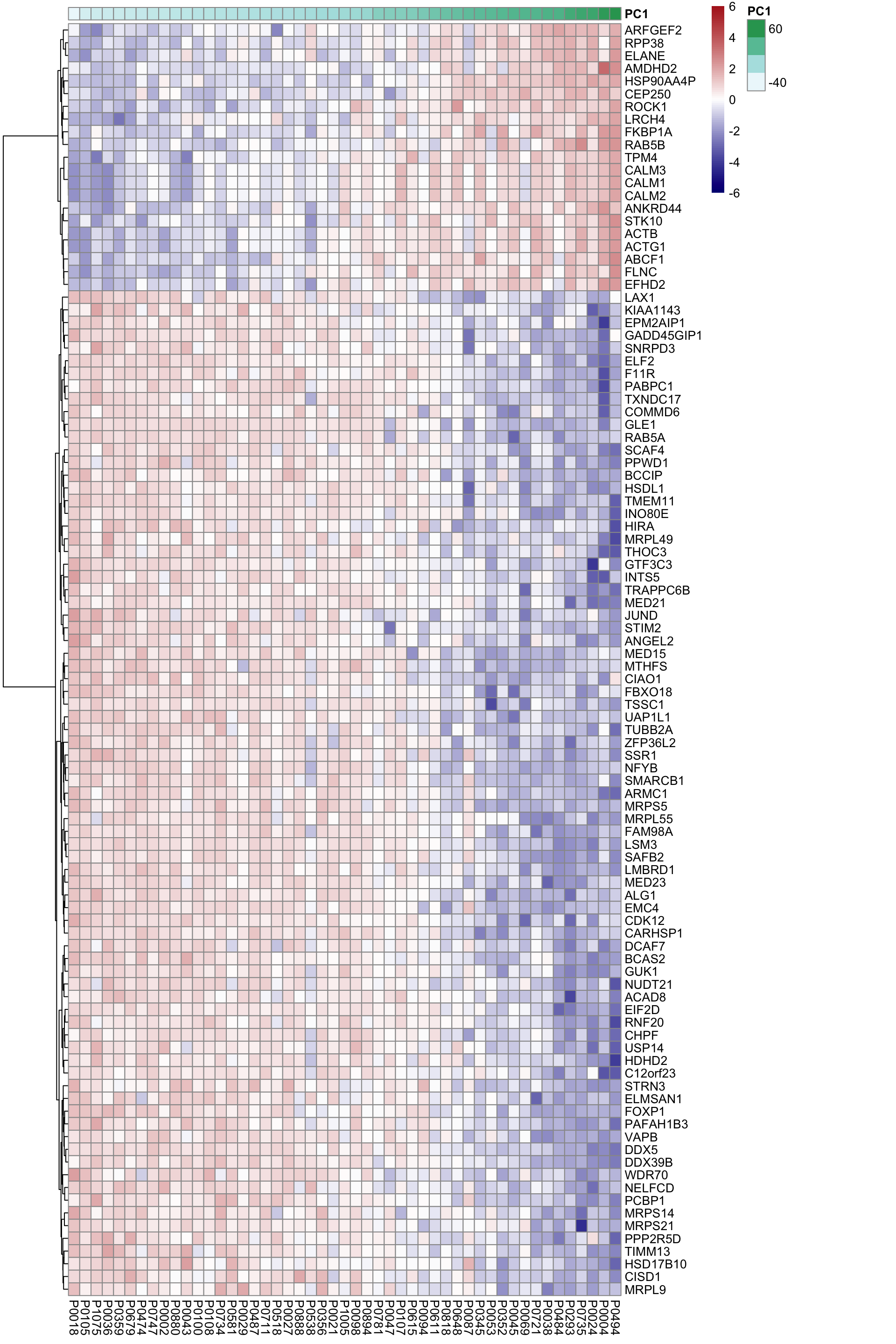
Enrichment using Camera
Hallmarks
gmts = list(H= "../data/gmts/h.all.v6.2.symbols.gmt",
            C6 = "../data/gmts/c6.all.v6.2.symbols.gmt",
            KEGG = "../data/gmts/c2.cp.kegg.v6.2.symbols.gmt")

res <- runCamera(proMat, designMat, gmts$H, id = rowData(protCLL[rownames(proMat),])$hgnc_symbol)
res$enrichPlot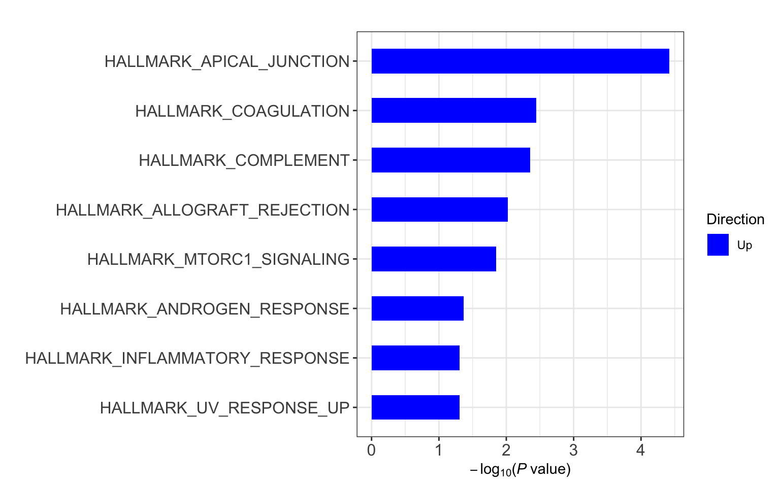
C6
res <- runCamera(proMat, designMat, gmts$C6, id = rowData(protCLL[rownames(proMat),])$hgnc_symbol)
res$enrichPlot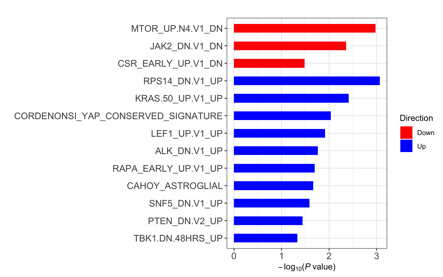
Annotate PC2
Correlation test
Assocation test
proMat <- assays(protCLL)[["QRILC"]]
pc <- pcRes[,2][colnames(proMat)]
designMat <- model.matrix(~1+pc)
fit <- lmFit(proMat,  designMat)
fit2 <- eBayes(fit)
corRes.pc2 <- topTable(fit2, number ="all", adjust.method = "BH", coef = "pc") %>% rownames_to_column("id") %>%
    mutate(symbol = rowData(protCLL[id,])$hgnc_symbol)
Number of significant associations (10% FDR)
hist(corRes.pc2$P.Value,breaks=100)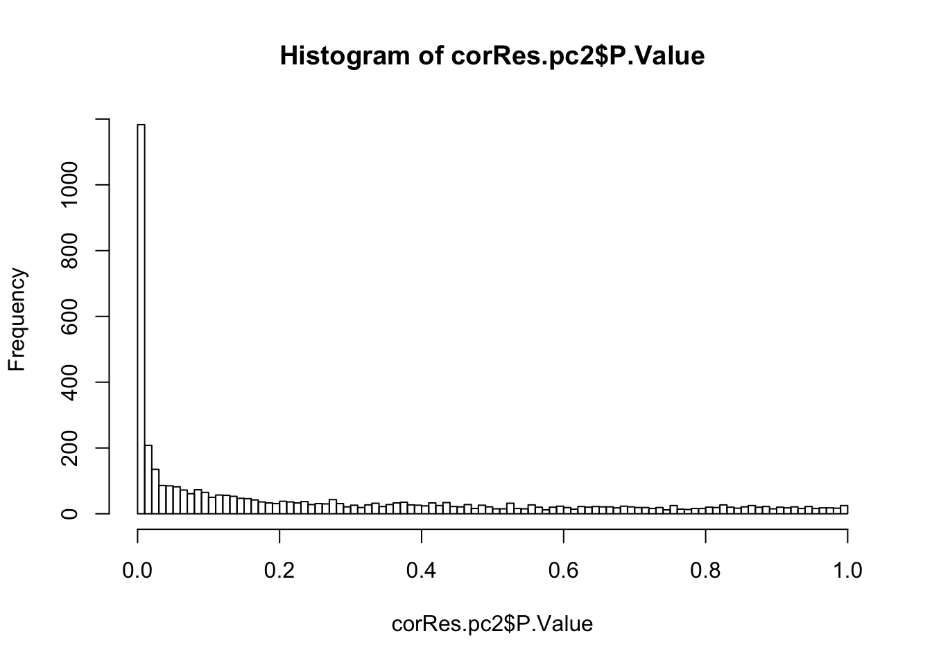
Table of significant associations (5% FDR)
resTab.sig <- filter(corRes.pc2, adj.P.Val < 0.05) %>%
  select(symbol, id,logFC, P.Value, adj.P.Val) %>%
  arrange(P.Value)
resTab.sig %>% mutate_if(is.numeric, formatC, digits=2, format= "e") %>%
  DT::datatable()
Heatmap of associated genes
colAnno <- tibble(patID = colnames(proMat), PC2 = pcRes[colnames(proMat),2]) %>%
  arrange(PC2) %>% data.frame() %>% column_to_rownames("patID")

plotMat <- proMat[resTab.sig$id[1:100],rownames(colAnno)]
plotMat <- jyluMisc::mscale(plotMat, censor = 6)

pheatmap(plotMat, scale = "none", annotation_col = colAnno, clustering_method = "ward.D2",
         cluster_cols = FALSE,
         labels_row = resTab.sig$symbol[1:100], color = colorRampPalette(c("navy","white","firebrick"))(100),
         breaks = seq(-6,6, length.out = 101))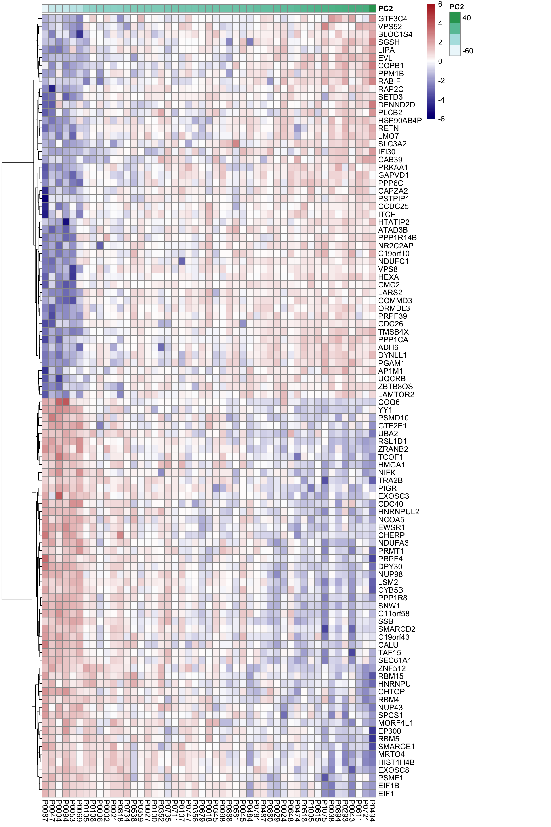
Enrichment using Camera
res <- runCamera(proMat, designMat, gmts$H, id = rowData(protCLL[rownames(proMat),])$hgnc_symbol)
res$enrichPlot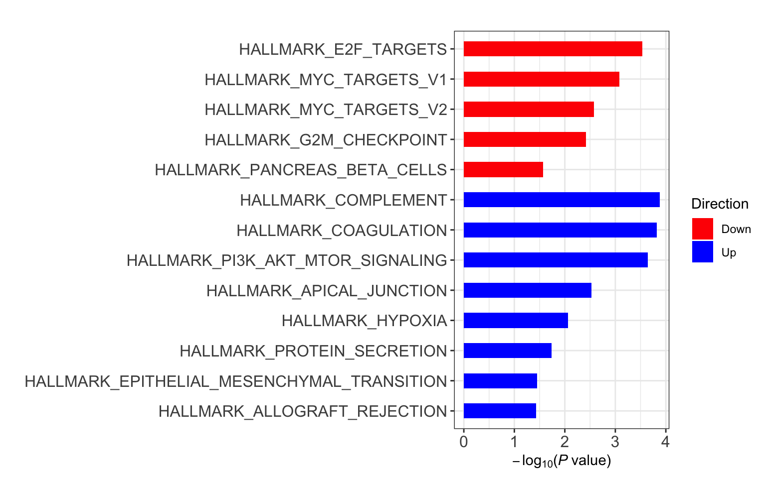
Association with lymphocyte count (potential contamination?)
load("~/CLLproject_jlu/ShinyApps/sampleTimeline//timeline.RData")
plotTab <- pcRes[,1:9] %>% data.frame()  %>%
  rownames_to_column("patID") %>% as_tibble() %>%
  mutate(sampleID = protCLL[,patID]$sampleID) %>%
  mutate(lymCount = sampleTab[match(sampleID, sampleTab$sampleID),]$leukCount) %>%
  gather(key = "pc", value = "val",-patID,-sampleID,-lymCount)

ggplot(plotTab, aes(x=val, y=lymCount)) + geom_point() + geom_smooth(method = "lm") +
  facet_wrap(~pc, ncol =3, scale = "free")
`geom_smooth()` using formula 'y ~ x'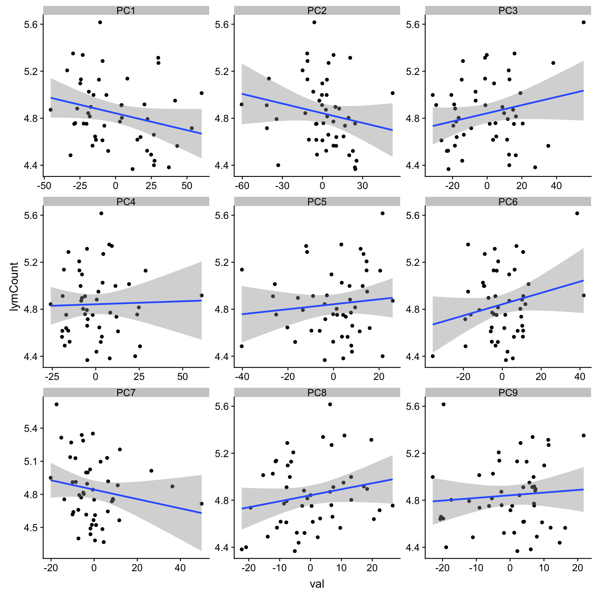
corRes <- plotTab %>% group_by(pc) %>% nest() %>%
  mutate(m= map(data, ~cor.test(~ val+ lymCount,.))) %>%
  mutate(res = map(m, broom::tidy)) %>%
  unnest(res) %>% select(pc, estimate, p.value) %>%
  arrange(p.value)
corRes
# A tibble: 9 x 3
# Groups: pc [9]
pc estimate p.value
<chr> <dbl> <dbl>
1 PC1 -0.253 0.0789
2 PC3 0.228 0.115
3 PC6 0.219 0.130
4 PC8 0.206 0.156
5 PC2 -0.194 0.182
6 PC7 -0.183 0.209
7 PC5 0.110 0.451
8 PC9 0.0840 0.566
9 PC4 0.0284 0.847 Association wit %Lymphocyte PB
library(DBI)

con <- dbConnect(RPostgreSQL::PostgreSQL(),
                 dbname = "tumorbank",
                 host = "huber-vm01.embl.de",
                 user = "admin",
                 password = "bloodcancertumorbank")

PBtab <- tbl(con, "patient") %>%
  left_join(tbl(con, "sample"), by = c(patid = "smppatidref")) %>%
  left_join(tbl(con, "analysis"), by = c(smpid = "anlsmpidref")) %>%
  collect() %>%
  select(patpatientid, smpsampleid, smpleukocytes, smpsampledate, smppblymphocytes)

dbDisconnect(con)
[1] TRUEplotTab <- pcRes[,1:9] %>% data.frame() %>%
rownames_to_column("patID") %>% as_tibble() %>%
mutate(sampleID = protCLL[,patID]$sampleID) %>%
mutate(perPB = PBtab[match(sampleID, PBtab$smpsampleid),]$smppblymphocytes) %>%
gather(key = "pc", value = "val",-patID,-sampleID,-perPB)
ggplot(plotTab, aes(x=val, y=perPB)) + geom_point() + geom_smooth(method = "lm") +
facet_wrap(~pc, ncol =3, scale = "free")`geom_smooth()` using formula 'y ~ x'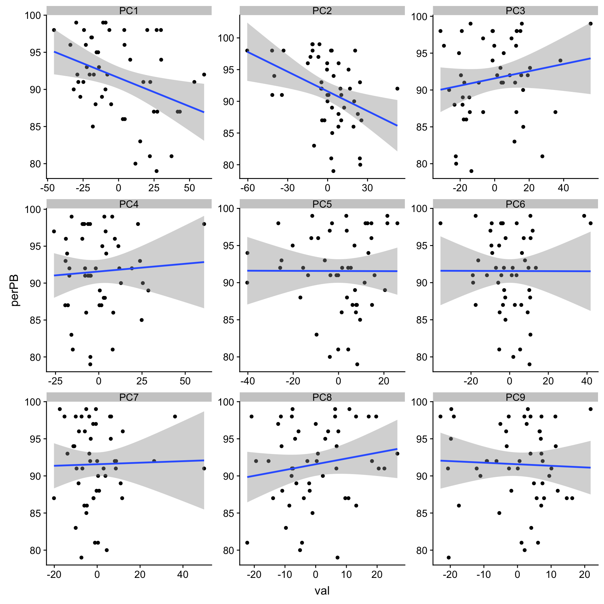
corRes <- plotTab %>% group_by(pc) %>% nest() %>%
  mutate(m= map(data, ~cor.test(~ val+ perPB,.))) %>%
  mutate(res = map(m, broom::tidy)) %>%
  unnest(res) %>% select(pc, estimate, p.value) %>%
  arrange(p.value)
corRes
# A tibble: 9 x 3
# Groups: pc [9]
pc estimate p.value
<chr> <dbl> <dbl>
1 PC2 -0.388 0.00586
2 PC1 -0.360 0.0110
3 PC3 0.171 0.240
4 PC8 0.165 0.256
5 PC4 0.0617 0.674
6 PC9 -0.0415 0.777
7 PC7 0.0235 0.872
8 PC5 -0.00258 0.986
9 PC6 -0.00207 0.989 Will the correlation with transcriptomics increase if PC1&2 are regressed out?
pc1 <- pcRes[colnames(rnaMat),1]
pc2 <- pcRes[colnames(rnaMat),2]

corTab <- lapply(geneOverlap, function(n) {
  rna <- rnaMat[n,]
  pro.q <- proMat.qrilc[n,]
  p.single <- anova(lm(rna ~ pro.q))$`Pr(>F)`[1]
  p.multi <- car::Anova(lm(rna ~ pro.q + pc1 + pc2))$`Pr(>F)`[1]
  tibble(name = n, corrected = c("no","yes"),
         p = c(p.single, p.multi))
}) %>% bind_rows() %>% mutate(p.adj = p.adjust(p, method = "BH")) %>% arrange(p)
Number of significant correlations VS FDR cut-off
plotTab <- lapply(seq(0,0.1, length.out = 100), function(fdr) {
  filTab <- dplyr::filter(corTab, p.adj < fdr) %>%
    group_by(corrected) %>% summarise(n = length(name)) %>% mutate(fdr = fdr)
}) %>% bind_rows()

ggplot(plotTab, aes(x=fdr, y = n, col = corrected))+ geom_line() +
  ylab("Number of significant correlations") +
  xlab("FDR cut-off")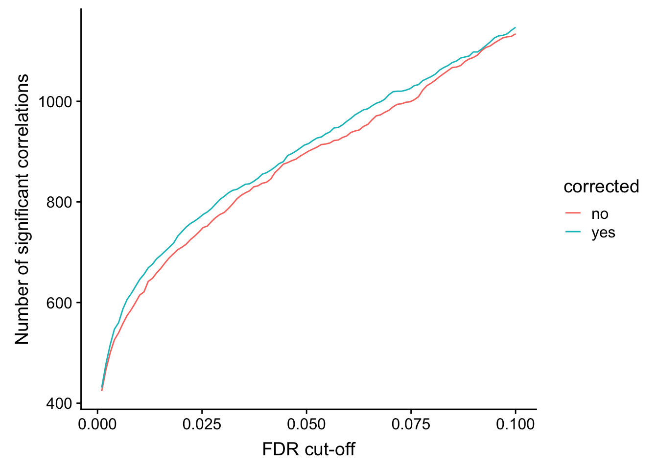
Seems to improve the correlation a little, but not much. We can include this factor in association test later.
Reconstruct data with PC1 and PC2 removed
protMat <- t(assays(protCLL)[["QRILC"]])
mu <- colMeans(protMat)

Xpca <- prcomp(protMat, center = TRUE, scale. = FALSE)

#reconstruct without the first two components
protMat.new <- Xpca$x[,3:ncol(Xpca$x)] %*% t(Xpca$rotation[,3:ncol(Xpca$x)])
protMat.new <- scale(protMat.new, center = -mu, scale = FALSE)

protMat.new <- t(protMat.new)
Hierarchical clustering using reconstructed matrix
plotMat <- protMat.new

colAnno <- colData(protCLL)[,c("gender","IGHV.status","trisomy12")] %>%
  data.frame()

plotMat <- jyluMisc::mscale(plotMat, censor = 6)
pheatmap(plotMat, scale = "none", annotation_col = colAnno, clustering_method = "ward.D2",
         show_rownames = FALSE, color = colorRampPalette(c("navy","white","firebrick"))(100),
         breaks = seq(-6,6, length.out = 101))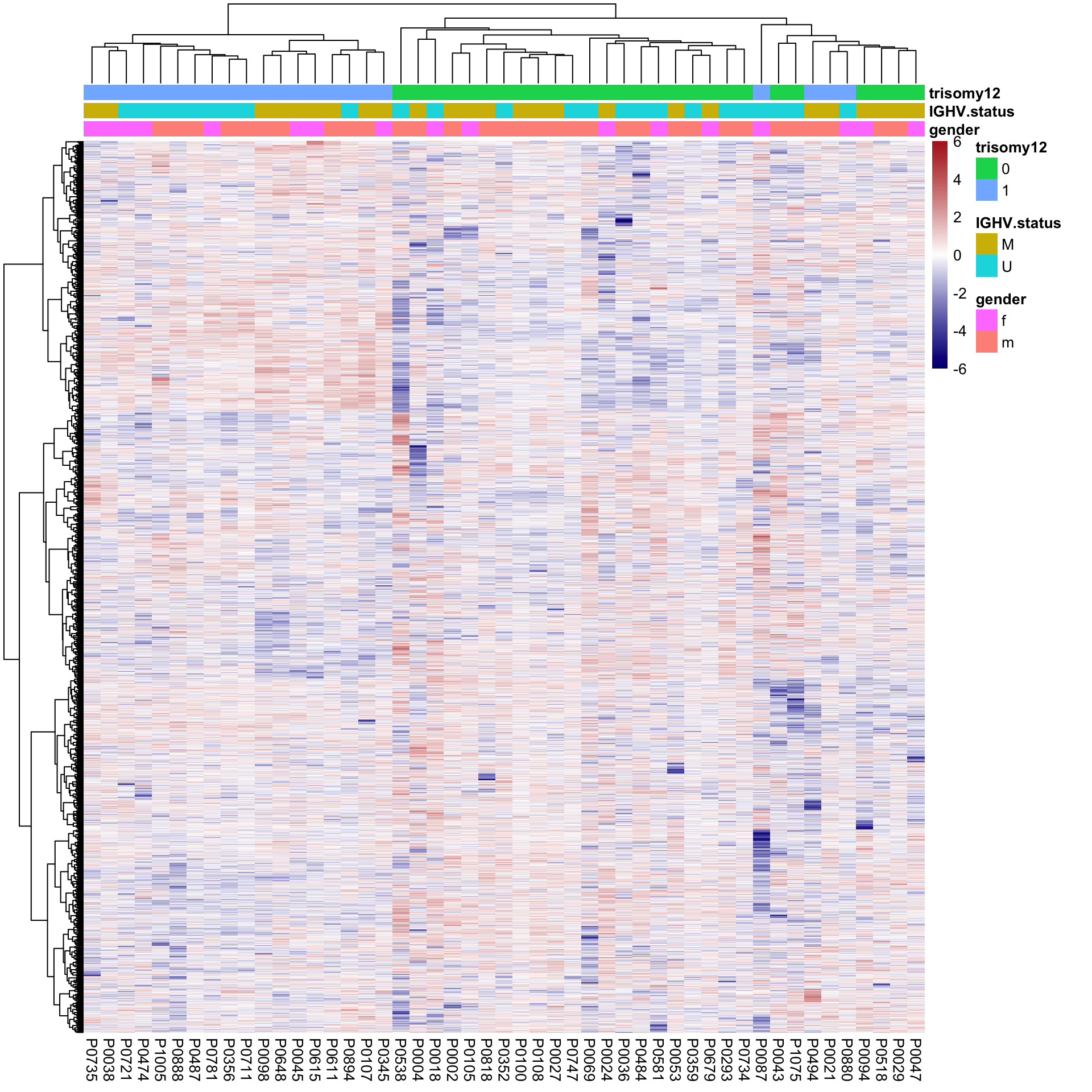
| Version | Author | Date |
|---|---|---|
| 8ba49d7 | Junyan Lu | 2020-03-17 |
Better separation for trisomy12 can be observed
PCA using reconstructed matrix
pcOut <- prcomp(t(plotMat), center =TRUE, scale. = FALSE)
pcRes.new <- pcOut$x
eigs <- pcOut$sdev^2
varExp <- structure(eigs/sum(eigs),names = colnames(pcRes.new))

plotTab <- pcRes.new[,1:2] %>% data.frame() %>% cbind(colAnno[rownames(.),]) %>%
  rownames_to_column("patID") %>% as_tibble()

ggplot(plotTab, aes(x=PC1, y=PC2, col = IGHV.status, shape = trisomy12)) + geom_point(size=4) +
  xlab(sprintf("PC1 (%1.2f%%)",varExp[["PC1"]]*100)) +
  ylab(sprintf("PC2 (%1.2f%%)",varExp[["PC2"]]*100))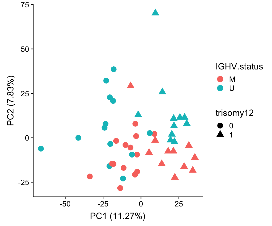
| Version | Author | Date |
|---|---|---|
| 8ba49d7 | Junyan Lu | 2020-03-17 |
Save the post process object
assays(protCLL)[["QRILC_re"]] <- protMat.new
protCLL$PC1 <- pcRes[colnames(protCLL),1]
protCLL$PC2 <- pcRes[colnames(protCLL),2]
save(protCLL, file = "../output/LUMOS_processed.RData")
sessionInfo()R version 3.6.0 (2019-04-26)
Platform: x86_64-apple-darwin15.6.0 (64-bit)
Running under: macOS 10.15.4
Matrix products: default
BLAS: /Library/Frameworks/R.framework/Versions/3.6/Resources/lib/libRblas.0.dylib
LAPACK: /Library/Frameworks/R.framework/Versions/3.6/Resources/lib/libRlapack.dylib
locale:
[1] en_US.UTF-8/en_US.UTF-8/en_US.UTF-8/C/en_US.UTF-8/en_US.UTF-8
attached base packages:
[1] parallel stats4 stats graphics grDevices utils datasets
[8] methods base
other attached packages:
[1] DBI_1.0.0 forcats_0.4.0
[3] stringr_1.4.0 dplyr_0.8.5
[5] purrr_0.3.3 readr_1.3.1
[7] tidyr_1.0.0 tibble_3.0.0
[9] tidyverse_1.3.0 DESeq2_1.24.0
[11] SummarizedExperiment_1.14.0 DelayedArray_0.10.0
[13] BiocParallel_1.18.0 matrixStats_0.54.0
[15] Biobase_2.44.0 GenomicRanges_1.36.0
[17] GenomeInfoDb_1.20.0 IRanges_2.18.1
[19] S4Vectors_0.22.0 BiocGenerics_0.30.0
[21] jyluMisc_0.1.5 pheatmap_1.0.12
[23] piano_2.0.2 cowplot_0.9.4
[25] ggplot2_3.3.0 limma_3.40.2
loaded via a namespace (and not attached):
[1] utf8_1.1.4 shinydashboard_0.7.1 tidyselect_1.0.0
[4] RSQLite_2.1.1 AnnotationDbi_1.46.0 htmlwidgets_1.3
[7] grid_3.6.0 maxstat_0.7-25 munsell_0.5.0
[10] codetools_0.2-16 DT_0.7 withr_2.1.2
[13] colorspace_1.4-1 knitr_1.23 rstudioapi_0.10
[16] ggsignif_0.5.0 labeling_0.3 git2r_0.26.1
[19] slam_0.1-45 GenomeInfoDbData_1.2.1 KMsurv_0.1-5
[22] bit64_0.9-7 farver_2.0.3 rprojroot_1.3-2
[25] vctrs_0.2.4 generics_0.0.2 TH.data_1.0-10
[28] xfun_0.8 sets_1.0-18 R6_2.4.0
[31] locfit_1.5-9.1 bitops_1.0-6 fgsea_1.10.0
[34] assertthat_0.2.1 promises_1.0.1 scales_1.1.0
[37] multcomp_1.4-10 nnet_7.3-12 gtable_0.3.0
[40] sandwich_2.5-1 workflowr_1.6.0 rlang_0.4.5
[43] genefilter_1.66.0 cmprsk_2.2-8 splines_3.6.0
[46] acepack_1.4.1 broom_0.5.2 checkmate_2.0.0
[49] yaml_2.2.0 abind_1.4-5 modelr_0.1.5
[52] crosstalk_1.0.0 backports_1.1.4 httpuv_1.5.1
[55] Hmisc_4.2-0 tools_3.6.0 relations_0.6-8
[58] RPostgreSQL_0.6-2 ellipsis_0.2.0 gplots_3.0.1.1
[61] RColorBrewer_1.1-2 Rcpp_1.0.1 base64enc_0.1-3
[64] visNetwork_2.0.7 zlibbioc_1.30.0 RCurl_1.95-4.12
[67] ggpubr_0.2.1 rpart_4.1-15 zoo_1.8-6
[70] ggrepel_0.8.1 haven_2.2.0 cluster_2.1.0
[73] exactRankTests_0.8-30 fs_1.4.0 magrittr_1.5
[76] data.table_1.12.2 openxlsx_4.1.0.1 reprex_0.3.0
[79] survminer_0.4.4 mvtnorm_1.0-11 whisker_0.3-2
[82] hms_0.5.2 shinyjs_1.0 mime_0.7
[85] evaluate_0.14 xtable_1.8-4 XML_3.98-1.20
[88] rio_0.5.16 readxl_1.3.1 gridExtra_2.3
[91] compiler_3.6.0 KernSmooth_2.23-15 crayon_1.3.4
[94] htmltools_0.4.0 mgcv_1.8-28 later_0.8.0
[97] Formula_1.2-3 geneplotter_1.62.0 lubridate_1.7.4
[100] dbplyr_1.4.2 MASS_7.3-51.4 Matrix_1.2-17
[103] car_3.0-3 cli_1.1.0 marray_1.62.0
[106] gdata_2.18.0 igraph_1.2.4.1 pkgconfig_2.0.2
[109] km.ci_0.5-2 foreign_0.8-71 xml2_1.2.2
[112] annotate_1.62.0 XVector_0.24.0 drc_3.0-1
[115] rvest_0.3.5 digest_0.6.19 rmarkdown_1.13
[118] cellranger_1.1.0 fastmatch_1.1-0 survMisc_0.5.5
[121] htmlTable_1.13.1 curl_3.3 shiny_1.3.2
[124] gtools_3.8.1 lifecycle_0.2.0 nlme_3.1-140
[127] jsonlite_1.6 carData_3.0-2 fansi_0.4.0
[130] pillar_1.4.3 lattice_0.20-38 httr_1.4.1
[133] plotrix_3.7-6 survival_2.44-1.1 glue_1.3.2
[136] zip_2.0.2 bit_1.1-14 stringi_1.4.3
[139] blob_1.1.1 latticeExtra_0.6-28 caTools_1.17.1.2
[142] memoise_1.1.0