Quality control of the proteomic data from LUMOS machine
Junyan Lu
2020-02-27
Last updated: 2020-12-03
Checks: 6 1
Knit directory: Proteomics/analysis/
This reproducible R Markdown analysis was created with workflowr (version 1.6.2). The Checks tab describes the reproducibility checks that were applied when the results were created. The Past versions tab lists the development history.
The R Markdown is untracked by Git. To know which version of the R Markdown file created these results, you'll want to first commit it to the Git repo. If you're still working on the analysis, you can ignore this warning. When you're finished, you can run wflow_publish to commit the R Markdown file and build the HTML.
Great job! The global environment was empty. Objects defined in the global environment can affect the analysis in your R Markdown file in unknown ways. For reproduciblity it's best to always run the code in an empty environment.
The command set.seed(20200227) was run prior to running the code in the R Markdown file. Setting a seed ensures that any results that rely on randomness, e.g. subsampling or permutations, are reproducible.
Great job! Recording the operating system, R version, and package versions is critical for reproducibility.
Nice! There were no cached chunks for this analysis, so you can be confident that you successfully produced the results during this run.
Great job! Using relative paths to the files within your workflowr project makes it easier to run your code on other machines.
Great! You are using Git for version control. Tracking code development and connecting the code version to the results is critical for reproducibility.
The results in this page were generated with repository version 3fb50c5. See the Past versions tab to see a history of the changes made to the R Markdown and HTML files.
Note that you need to be careful to ensure that all relevant files for the analysis have been committed to Git prior to generating the results (you can use wflow_publish or wflow_git_commit). workflowr only checks the R Markdown file, but you know if there are other scripts or data files that it depends on. Below is the status of the Git repository when the results were generated:
Ignored files:
    Ignored:    .DS_Store
    Ignored:    .Rhistory
    Ignored:    .Rproj.user/
    Ignored:    analysis/.DS_Store
    Ignored:    analysis/.Rhistory
    Ignored:    analysis/correlateCLLPD_cache/
    Ignored:    analysis/figure/
    Ignored:    analysis/lassoForSTAT2_cache/
    Ignored:    analysis/manuscript_S1_Overview_cache/
    Ignored:    analysis/manuscript_S1_Overview_presentation_cache/
    Ignored:    analysis/manuscript_S2_genomicAssociation_oldTimsTOF_cache/
    Ignored:    analysis/manuscript_S3_trisomy12_cache/
    Ignored:    analysis/manuscript_S4_IGHV_cache/
    Ignored:    analysis/manuscript_S4_IGHV_oldTimsTOF_cache/
    Ignored:    analysis/manuscript_S5_trisomy19_cache/
    Ignored:    analysis/manuscript_S6_del11q_cache/
    Ignored:    analysis/manuscript_S6_del11q_oldTimsTOF_cache/
    Ignored:    analysis/manuscript_S7_SF3B1_cache/
    Ignored:    analysis/manuscript_S8_drugResponse_Outcomes_cache/
    Ignored:    analysis/manuscript_S9_STAT2_cache/
    Ignored:    code/.Rhistory
    Ignored:    data/.DS_Store
    Ignored:    output/.DS_Store

Untracked files:
    Untracked:  analysis/.trisomy12_norm.pdf
    Untracked:  analysis/CNVanalysis_11q.Rmd
    Untracked:  analysis/CNVanalysis_trisomy12.Rmd
    Untracked:  analysis/CNVanalysis_trisomy19.Rmd
    Untracked:  analysis/STAT2_cytokines.Rmd
    Untracked:  analysis/SUGP1_splicing.svg.xml
    Untracked:  analysis/analysisDrugResponses.Rmd
    Untracked:  analysis/analysisDrugResponses_IC50.Rmd
    Untracked:  analysis/analysisPCA.Rmd
    Untracked:  analysis/analysisPreliminary_LUMOS.Rmd
    Untracked:  analysis/analysisPreliminary_timsTOF_Hela.Rmd
    Untracked:  analysis/analysisPreliminary_timsTOF_new.Rmd
    Untracked:  analysis/analysisSplicing.Rmd
    Untracked:  analysis/analysisTrisomy19.Rmd
    Untracked:  analysis/annotateCNV.Rmd
    Untracked:  analysis/comparePlatforms_LUMOS_helaTimsTOF.Rmd
    Untracked:  analysis/comparePlatforms_LUMOS_newTimsTOF.Rmd
    Untracked:  analysis/comparePlatforms_newTimsTOF_helaTimsTOF.Rmd
    Untracked:  analysis/complexAnalysis_IGHV.Rmd
    Untracked:  analysis/complexAnalysis_IGHV_alternative.Rmd
    Untracked:  analysis/complexAnalysis_overall.Rmd
    Untracked:  analysis/complexAnalysis_trisomy12.Rmd
    Untracked:  analysis/complexAnalysis_trisomy12_alternative.Rmd
    Untracked:  analysis/correlateGenomic_PC12adjusted.Rmd
    Untracked:  analysis/correlateGenomic_noBlock.Rmd
    Untracked:  analysis/correlateGenomic_noBlock_MCLL.Rmd
    Untracked:  analysis/correlateGenomic_noBlock_UCLL.Rmd
    Untracked:  analysis/correlateGenomic_timsTOFnew.Rmd
    Untracked:  analysis/correlateGenomic_timsTOFnewHela.Rmd
    Untracked:  analysis/correlateRNAexpression.Rmd
    Untracked:  analysis/default.css
    Untracked:  analysis/del11q.pdf
    Untracked:  analysis/del11q_norm.pdf
    Untracked:  analysis/full_diff_list.csv
    Untracked:  analysis/lassoForSTAT2.Rmd
    Untracked:  analysis/manuscript_S0_PrepareData.Rmd
    Untracked:  analysis/manuscript_S1_Overview.Rmd
    Untracked:  analysis/manuscript_S2_genomicAssociation.Rmd
    Untracked:  analysis/manuscript_S2_genomicAssociation_oldTimsTOF.Rmd
    Untracked:  analysis/manuscript_S3_trisomy12.Rmd
    Untracked:  analysis/manuscript_S4_IGHV.Rmd
    Untracked:  analysis/manuscript_S4_IGHV_oldTimsTOF.Rmd
    Untracked:  analysis/manuscript_S5_trisomy19.Rmd
    Untracked:  analysis/manuscript_S6_del11q.Rmd
    Untracked:  analysis/manuscript_S6_del11q_oldTimsTOF.Rmd
    Untracked:  analysis/manuscript_S7_SF3B1.Rmd
    Untracked:  analysis/manuscript_S8_drugResponse_Outcomes.Rmd
    Untracked:  analysis/manuscript_S9_STAT2.Rmd
    Untracked:  analysis/peptideValidate.Rmd
    Untracked:  analysis/plotCNV_del11q.pdf
    Untracked:  analysis/plotExpressionCNV.Rmd
    Untracked:  analysis/processPeptides_LUMOS.Rmd
    Untracked:  analysis/processProteomics_new.Rmd
    Untracked:  analysis/processProteomics_timsTOF_Hela.Rmd
    Untracked:  analysis/processProteomics_timsTOF_new.Rmd
    Untracked:  analysis/protCLL.RData
    Untracked:  analysis/qualityControl_LUMOSnew.Rmd
    Untracked:  analysis/qualityControl_timsTOF_Hela.Rmd
    Untracked:  analysis/qualityControl_timsTOF_new.Rmd
    Untracked:  analysis/style.css
    Untracked:  analysis/tableS1_DE_proteins_p0.01.xlsx
    Untracked:  analysis/test.pdf
    Untracked:  analysis/test.svg
    Untracked:  analysis/tri12Enrich.pdf
    Untracked:  analysis/trisomy12.pdf
    Untracked:  analysis/trisomy12_AFcor.Rmd
    Untracked:  analysis/trisomy12_norm.pdf
    Untracked:  analysis/uniprotIDs.txt
    Untracked:  code/AlteredPQR.R
    Untracked:  code/utils.R
    Untracked:  data/190909_CLL_prot_abund_med_norm.tsv
    Untracked:  data/190909_CLL_prot_abund_no_norm.tsv
    Untracked:  data/200725_cll_diaPASEF_direct_reports/
    Untracked:  data/200728_cll_diaPASEF_direct_plus_hela_reports/
    Untracked:  data/20190423_Proteom_submitted_samples_bereinigt.xlsx
    Untracked:  data/20191025_Proteom_submitted_samples_final.xlsx
    Untracked:  data/20201120_p3254_o23219_SpectronautReports/
    Untracked:  data/Chemokines.csv
    Untracked:  data/IFN_list.csv
    Untracked:  data/IFNreceptor.csv
    Untracked:  data/Interleukin_receptor.csv
    Untracked:  data/Interleukins.csv
    Untracked:  data/LUMOS/
    Untracked:  data/LUMOS_peptides/
    Untracked:  data/LUMOS_protAnnotation.csv
    Untracked:  data/LUMOS_protAnnotation_fix.csv
    Untracked:  data/SampleAnnotation_cleaned.xlsx
    Untracked:  data/chemoReceptor.csv
    Untracked:  data/example_proteomics_data
    Untracked:  data/facTab_CPSatLeast3New.RData
    Untracked:  data/gmts/
    Untracked:  data/mapEnsemble.txt
    Untracked:  data/mapSymbol.txt
    Untracked:  data/proteins_in_complexes
    Untracked:  data/pyprophet_export_aligned.csv
    Untracked:  data/timsTOF_protAnnotation.csv
    Untracked:  output/Figure1A.png
    Untracked:  output/Figure1A.pptx
    Untracked:  output/LUMOS_processed.RData
    Untracked:  output/LUMOSnew_processed.RData
    Untracked:  output/MSH6_splicing.svg
    Untracked:  output/SUGP1_splicing.eps
    Untracked:  output/SUGP1_splicing.pdf
    Untracked:  output/SUGP1_splicing.svg
    Untracked:  output/cnv_plots.zip
    Untracked:  output/cnv_plots/
    Untracked:  output/cnv_plots_norm.zip
    Untracked:  output/ddsrna_enc.RData
    Untracked:  output/deResList.RData
    Untracked:  output/deResList_timsTOF.RData
    Untracked:  output/deResList_timsTOF_old.RData
    Untracked:  output/dxdCLL.RData
    Untracked:  output/dxdCLL2.RData
    Untracked:  output/encMap.RData
    Untracked:  output/exprCNV.RData
    Untracked:  output/exprCNV_enc.RData
    Untracked:  output/lassoResults_CPS.RData
    Untracked:  output/lassoResults_IC50.RData
    Untracked:  output/patMeta_enc.RData
    Untracked:  output/pepCLL_lumos.RData
    Untracked:  output/pepCLL_lumos_enc.RData
    Untracked:  output/pepTab_lumos.RData
    Untracked:  output/pheno1000_enc.RData
    Untracked:  output/pheno1000_main.RData
    Untracked:  output/plotCNV_allChr11_diff.pdf
    Untracked:  output/plotCNV_del11q_sum.pdf
    Untracked:  output/proteomic_LUMOS_20200227.RData
    Untracked:  output/proteomic_LUMOS_20200320.RData
    Untracked:  output/proteomic_LUMOS_20200430.RData
    Untracked:  output/proteomic_LUMOS_enc.RData
    Untracked:  output/proteomic_newLUMOS_20201124.RData
    Untracked:  output/proteomic_timsTOF_20200227.RData
    Untracked:  output/proteomic_timsTOF_Hela_20200806.RData
    Untracked:  output/proteomic_timsTOF_enc.RData
    Untracked:  output/proteomic_timsTOF_new_20200806.RData
    Untracked:  output/proteomic_timsTOF_old_enc.RData
    Untracked:  output/splicingResults.RData
    Untracked:  output/survival_enc.RData
    Untracked:  output/timsTOF_processed.RData
    Untracked:  plotCNV_del11q_diff.pdf
    Untracked:  summary/
    Untracked:  supp_latex/

Unstaged changes:
    Modified:   analysis/_site.yml
    Modified:   analysis/analysisSF3B1.Rmd
    Modified:   analysis/compareProteomicsRNAseq.Rmd
    Modified:   analysis/correlateCLLPD.Rmd
    Modified:   analysis/correlateGenomic.Rmd
    Deleted:    analysis/correlateGenomic_removePC.Rmd
    Modified:   analysis/correlateMIR.Rmd
    Modified:   analysis/correlateMethylationCluster.Rmd
    Modified:   analysis/index.Rmd
    Modified:   analysis/predictOutcome.Rmd
    Modified:   analysis/processProteomics_LUMOS.Rmd
    Modified:   analysis/qualityControl_LUMOS.Rmd
Note that any generated files, e.g. HTML, png, CSS, etc., are not included in this status report because it is ok for generated content to have uncommitted changes.
There are no past versions. Publish this analysis with wflow_publish() to start tracking its development.
Test association with RNA expression
Dimension of the inputed data
dim(protCLL)[1] 3487 48Process both datasets
colnames(dds) <- dds$PatID
dds <- estimateSizeFactors(dds)
sampleOverlap <- intersect(colnames(protCLL), colnames(dds))
geneOverlap <- intersect(rowData(protCLL)$ensembl_gene_id, rownames(dds))
ddsSub <- dds[geneOverlap, sampleOverlap]
protSub <- protCLL[match(geneOverlap, rowData(protCLL)$ensembl_gene_id), sampleOverlap]

#how many gene don't have RNA expression at all?
noExp <- rowSums(counts(ddsSub)) == 0
sum(noExp)
[1] 50#remove those genes in both datasets
ddsSub <- ddsSub[!noExp,]
protSub <- protSub[!noExp,]
#remove proteins with duplicated identifiers
protSub <- protSub[!duplicated(rowData(protSub)$name)]
geneOverlap <- intersect(rowData(protSub)$ensembl_gene_id, rownames(ddsSub))
ddsSub.vst <- varianceStabilizingTransformation(ddsSub)How many overlapped samples?
length(sampleOverlap)[1] 32Calculate correlations between protein abundance and RNA expression
rnaMat <- assay(ddsSub.vst)
proMat.raw <- assays(protSub)[["count"]]
proMat.qrilc <- assays(protSub)[["QRILC"]]
rownames(proMat.qrilc) <- rowData(protSub)$ensembl_gene_id
rownames(proMat.raw) <- rowData(protSub)$ensembl_gene_id

corTab <- lapply(geneOverlap, function(n) {
  rna <- rnaMat[n,]
  pro.q <- proMat.qrilc[n,]
  pro.raw <- proMat.raw[n,]
  res.q <- cor.test(rna, pro.q)
  res.raw <- cor.test(rna, pro.raw, use = "pairwise.complete.obs")
  tibble(id = n, impute=c("No Imputation","QRILC"),
         p = c(res.raw$p.value, res.q$p.value),
         coef = c(res.raw$estimate, res.q$estimate))
}) %>% bind_rows() %>%
  arrange(desc(coef)) %>% mutate(p.adj = p.adjust(p, method = "BH"),
                                 symbol = rowData(dds[id,])$symbol)
Plot the distribution of correlation coefficient
ggplot(corTab, aes(x=coef, fill = impute)) + geom_histogram(position = "identity", col = "grey50", alpha =0.3, bins =100) +
geom_vline(xintercept = 0, col = "red", linetype = "dashed")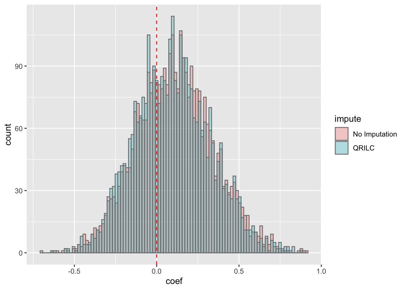 Most of the correlations are positive, which is reasonable.
Number of significant positive and negative correlations (10% FDR)
sigTab <- corTab %>% filter(p.adj < 0.1) %>% mutate(direction = ifelse(coef > 0, "positive", "negative")) %>%
  group_by(impute, direction) %>% summarise(number = length(id)) %>% ungroup() %>%
  mutate(ratio = format(number/length(geneOverlap), digits = 2)) %>% arrange(number)
DT::datatable(sigTab)
Number of significant correlations VS FDR cut-off
plotTab <- lapply(seq(0,0.1, length.out = 100), function(fdr) {
  filTab <- dplyr::filter(corTab, p.adj < fdr, coef > 0) %>%
    group_by(impute) %>% summarise(n = length(id)) %>% mutate(fdr = fdr)
}) %>% bind_rows()

ggplot(plotTab, aes(x=fdr, y = n, col = impute))+ geom_line() +
  ylab("Number of significant correlations") +
  xlab("FDR cut-off")
List of proteins that significantly correlated with RNA expression (10 %FDR, no imputation)
sigTab <- filter(corTab, p.adj < 0.1, impute == "No Imputation") %>% mutate_if(is.numeric, format, digits=2)
DT::datatable(sigTab)
List of proteins that significantly correlated with RNA expression (10 %FDR, QRILC imputed)
sigTab <- filter(corTab, p.adj < 0.1, impute == "QRILC") %>% mutate_if(is.numeric, format, digits=2)
DT::datatable(sigTab)
Correlation plot of top 9 most correlated protein-rna pairs
plotList <- lapply(sigTab$id[1:9], function(n) {
  plotTab <- tibble(pro = proMat.qrilc[n,], gene = rnaMat[n,])
  symbol <- filter(sigTab, id == n)$symbol
  ggplot(plotTab, aes(x=pro, y=gene)) + geom_point() + geom_smooth(method = "lm") +
    ggtitle(symbol) + ylab("RNA expression") + xlab("Protein abundance")
})

cowplot::plot_grid(plotlist = plotList, ncol =3)
Scater plot of protein pairs show significant correlations
idList <- filter(corTab, p.adj <= 0.1, coef > 0, impute == "No Imputation")$id
protTab.raw <- proMat.raw[idList, ] %>% data.frame() %>% rownames_to_column("id") %>%
  gather(key = "patID", value = "protein", -id)
rnaTab.raw <- rnaMat[idList, ] %>% data.frame() %>% rownames_to_column("id") %>%
  gather(key = "patID", value = "rna", -id)
plotTab <- left_join(protTab.raw, rnaTab.raw, by = c("patID","id"))
ggplot(plotTab, aes(x=rna, y = protein)) + geom_point(aes(col = patID), alpha =0.5) + geom_smooth(method = "lm")
Check data structure
Hierarchical clustering
load("../data/facTab_CPSatLeast3New.RData")

plotMat <- assays(protCLL)[["QRILC"]]

techFac <- colData(protCLL)[,c("processDate","Viability","viabBeforeSorting","viabAfterSorting")] %>%
  data.frame() %>% rownames_to_column("Patient.ID") %>%
  mutate(viabAfterSorting = as.numeric(viabAfterSorting),
         processDate = as.character(processDate))

patAnno <- filter(patMeta, Patient.ID %in% colnames(plotMat)) %>%
  select(Patient.ID, IGHV.status, gender)

colAnno <- left_join(techFac, patAnno) %>%
  mutate_if(is.factor,droplevels) %>%
  mutate(CLLPD = facTab[match(Patient.ID, facTab$patID),]$factor) %>%
  data.frame() %>% column_to_rownames("Patient.ID")

plotMat <- jyluMisc::mscale(plotMat, censor = 6)
pheatmap(plotMat, scale = "none", annotation_col = colAnno, clustering_method = "complete",
         show_rownames = FALSE, color = colorRampPalette(c("navy","white","firebrick"))(100),
         breaks = seq(-6,6, length.out = 101))
There's a clear cluster with low viability after sorting.
The patient with replicates (P0369, and P0369_2) are not groupped together.
PCA
pcOut <- prcomp(t(plotMat), center =TRUE, scale. = TRUE)
pcRes <- pcOut$x
eigs <- pcOut$sdev^2
varExp <- structure(eigs/sum(eigs),names = colnames(pcRes))

plotTab <- pcRes[,1:2] %>% data.frame() %>%
  rownames_to_column("patID") %>% as_tibble() %>%
  mutate(viabAfterSorting= colAnno[patID,]$viabAfterSorting )

ggplot(plotTab, aes(x=PC1, y=PC2, col = viabAfterSorting)) + geom_point(size=4) +
  xlab(sprintf("PC1 (%1.2f%%)",varExp[["PC1"]]*100)) +
  ylab(sprintf("PC2 (%1.2f%%)",varExp[["PC2"]]*100)) +
  ggrepel::geom_text_repel(aes(label = patID))
PC1 is associated with viability after sorting
Preproducibility between the replicates for P0369
Assocations
protRep <- protCLL[,c("P0369","P0369_2")]
plotTab <- assays(protRep)[["count"]] %>% data.frame()
ggplot(plotTab, aes(x=P0369,y=P0369_2)) + geom_point()
The global expression pattern of proteins are well correlated with the two replicates. But based on the PCA and heatmap, the two replicates are not more similar to each other than to the samples from other patients.
Missing values
missTab <- plotTab %>% mutate(miss = case_when(
  is.na(P0369) & is.na(P0369_2) ~ "both",
  is.na(P0369) & !is.na(P0369_2) ~ "only_rep1",
  !is.na(P0369) & is.na(P0369_2) ~ "only_rep2",
  TRUE ~ "none"
))
table(missTab$miss)
     both      none only_rep1 only_rep2
       19      3380        47        41
Here I will choose the second replicate for P0369, as it shows slightly less missing values.
protCLL <- protCLL[,colnames(protCLL) != "P0369"]
colnames(protCLL)[colnames(protCLL) == "P0369_2"] <- "P0369"
Assocation with technical factors
Are thechnical variables confounded with major genomic variabes?
# A tibble: 8 x 4
  genomic     technical           pval  p.adj
  <chr>       <chr>              <dbl>  <dbl>
1 SF3B1       Viability        0.00129 0.0273
2 IGHV.status Viability        0.00276 0.0273
3 del13q      Viability        0.00293 0.0273
4 TP53        Viability        0.00551 0.0386
5 U1          processDate      0.0193  0.108
6 del13q      viabAfterSorting 0.0332  0.148
7 U1          Viability        0.0422  0.148
8 IGHV.status viabAfterSorting 0.0422  0.148
SF3B1 versus Viability
plotTab <- tibble(gene = geneTab$SF3B1, Viability = techTab$Viability)
ggplot(plotTab, aes(x=gene, y = Viability)) + geom_boxplot() + geom_point()
There's a small trend that trisomy12 samples tend to have higher protein concentration.
Association between technical variables and priciple components of protein expression
plotMat <- assays(protCLL)[["QRILC"]]
pcRes <- prcomp(t(plotMat), center =TRUE, scale. = TRUE)$x
techTab$processDate <- NULL
testRes <- lapply(colnames(pcRes), function(pc) {
  lapply(colnames(techTab), function(tech) {
    pcVar <- pcRes[,pc]
    techVar <- techTab[[tech]]
    res <- cor.test(pcVar, techVar)
    p <- res$p.value
    tibble(component = pc, technical = tech, pval = p)
  }) %>% bind_rows()
}) %>% bind_rows() %>% mutate(p.adj = p.adjust(pval, method = "BH")) %>%
  arrange(pval)
filter(testRes, p.adj < 0.5)
# A tibble: 7 x 4
component technical pval p.adj
<chr> <chr> <dbl> <dbl>
1 PC10 Viability 0.000163 0.0230
2 PC1 viabAfterSorting 0.000536 0.0281
3 PC12 Viability 0.000598 0.0281
4 PC10 viabBeforeSorting 0.00171 0.0603
5 PC15 viabBeforeSorting 0.00297 0.0839
6 PC32 viabAfterSorting 0.0159 0.372
7 PC9 Viability 0.0222 0.446 Associations between technical variables and individual protein expressions
Association test
techTab <- colData(protCLL)[,c("Viability","viabAfterSorting")] %>%
  data.frame() %>%rownames_to_column("patID") %>% as_tibble() %>% mutate_at(vars(-patID), as.numeric)
testTab <- assays(protCLL)[["QRILC"]] %>% data.frame() %>%
  rownames_to_column("id") %>% mutate(name = rowData(protCLL)[id,]$hgnc_symbol) %>%
  gather(key = "patID", value = "expr", -id, -name) %>%
  left_join(techTab, by ="patID") %>% gather(key = technical, value = value, -id, -name, -patID, -expr)

testRes <- filter(testTab, !is.na(value)) %>%
  group_by(name, technical) %>% nest() %>%
  mutate(m = map(data, ~lm(expr~value,.))) %>%
  mutate(res = map(m, broom::tidy)) %>%
  unnest(res) %>% filter(term=="value") %>%
  ungroup() %>%
  mutate(p.adj = p.adjust(p.value, method = "BH"))

sumTab <- filter(testRes, p.adj < 0.1) %>% group_by(technical) %>% summarise(n=length(name))
ggplot(sumTab, aes(x=technical, y = n)) + geom_bar(stat = "identity") + coord_flip() +
  xlab("") + ylab("Number of significantly associated proteins")
Assocation P value histogram for each technical factor
ggplot(testRes, aes(x=p.value)) + geom_histogram() + facet_wrap(~technical, scale="free") + xlim(0,1) Also based on the p-value histogram, only overall protein concentration may have potential impact on protein abundance detection.
List of proteins that show significant correlation with total protein concentration (10% FDR)
filter(testRes, technical == "viabAfterSorting") %>% select(name, p.value, p.adj, estimate) %>%
  arrange(p.value) %>% filter(p.adj <= 0.1) %>%
  mutate_if(is.numeric, formatC, digits=2, format="e") %>%
  DT::datatable()
Will the correlation with RNA expression improve if we adjust for viab after sorting
viab <- techTab[match(colnames(proMat.qrilc), techTab$patID),]$viabAfterSorting
corTab <- lapply(geneOverlap, function(n) {
  rna <- rnaMat[n,]
  pro.q <- proMat.qrilc[n,]
  p.single <- anova(lm(rna ~ pro.q))$`Pr(>F)`[1]
  p.multi <- car::Anova(lm(rna ~ pro.q + viab))$`Pr(>F)`[1]
  tibble(name = n, corrected = c("no","yes"),
         p = c(p.single, p.multi))
}) %>% bind_rows() %>% mutate(p.adj = p.adjust(p, method = "BH")) %>% arrange(p)
Number of significant correlations VS FDR cut-off
plotTab <- lapply(seq(0,0.1, length.out = 100), function(fdr) {
filTab <- dplyr::filter(corTab, p.adj < fdr) %>%
group_by(corrected) %>% summarise(n = length(name)) %>% mutate(fdr = fdr)
}) %>% bind_rows()
ggplot(plotTab, aes(x=fdr, y = n, col = corrected))+ geom_line() +
ylab("Number of significant correlations") +
xlab("FDR cut-off")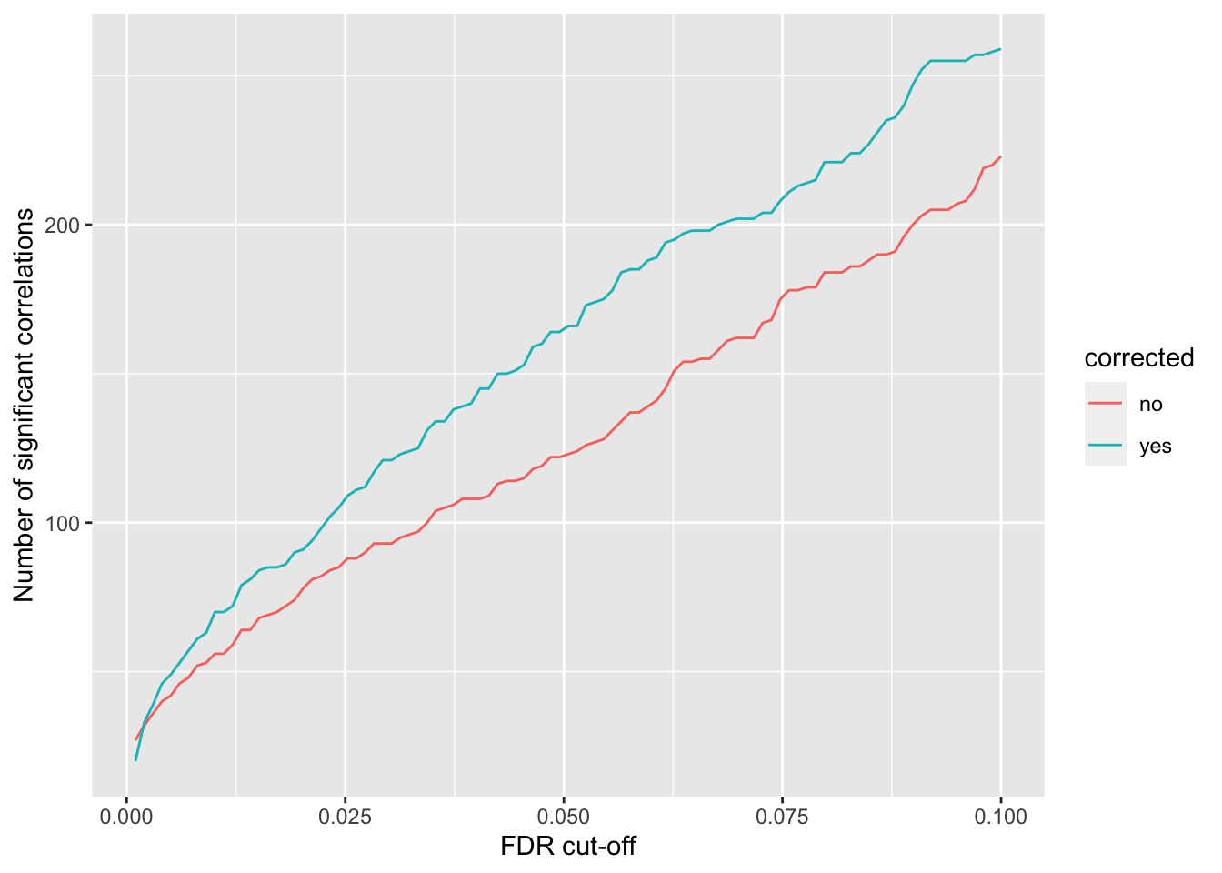 Seems to improve the correlation a little, but not much. We can include this factor in association test later.
Biological annotation of PC1 and PC2
Annotate PC1
Correlation test
Assocation test
proMat <- assays(protCLL)[["QRILC"]]
pc <- pcRes[,1][colnames(proMat)]
designMat <- model.matrix(~1+pc)
fit <- lmFit(proMat,  designMat)
fit2 <- eBayes(fit)
corRes.pc1 <- topTable(fit2, number ="all", adjust.method = "BH", coef = "pc") %>% rownames_to_column("id") %>%
    mutate(symbol = rowData(protCLL[id,])$hgnc_symbol)
Number of significant associations (10% FDR)
hist(corRes.pc1$P.Value,breaks=100)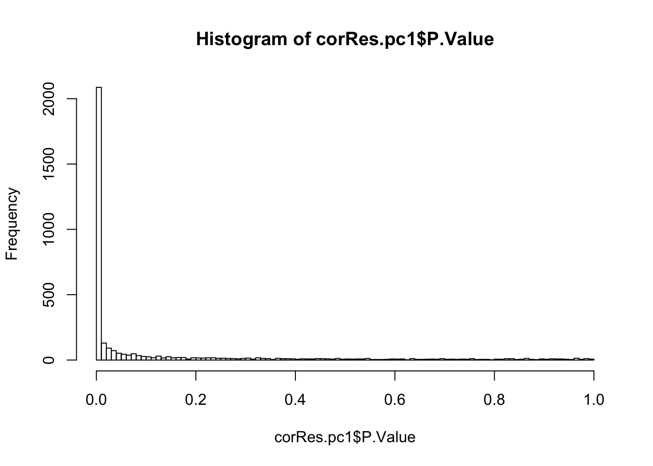
Table of significant associations (5% FDR)
resTab.sig <- filter(corRes.pc1, adj.P.Val < 0.05) %>%
  select(symbol, id,logFC, P.Value, adj.P.Val) %>%
  arrange(P.Value)
resTab.sig %>% mutate_if(is.numeric, formatC, digits=2, format= "e") %>%
  DT::datatable()
Heatmap of associated genes
colAnno <- tibble(patID = colnames(proMat), PC1 = pcRes[colnames(proMat),1]) %>%
  left_join(techTab) %>%
  arrange(PC1) %>% data.frame() %>% column_to_rownames("patID")

plotMat <- proMat[resTab.sig$id[1:200],rownames(colAnno)]
plotMat <- jyluMisc::mscale(plotMat, censor = 6)

pheatmap(plotMat, scale = "none", annotation_col = colAnno, clustering_method = "ward.D2",
         cluster_cols = FALSE,
         labels_row = resTab.sig$symbol[1:200], color = colorRampPalette(c("navy","white","firebrick"))(100),
         breaks = seq(-6,6, length.out = 101))
Enrichment using Camera
Hallmarks
gmts = list(H= "../data/gmts/h.all.v6.2.symbols.gmt",
            C6 = "../data/gmts/c6.all.v6.2.symbols.gmt",
            KEGG = "../data/gmts/c2.cp.kegg.v6.2.symbols.gmt")

res <- runCamera(proMat, designMat, gmts$H, id = rowData(protCLL[rownames(proMat),])$hgnc_symbol)
res$enrichPlot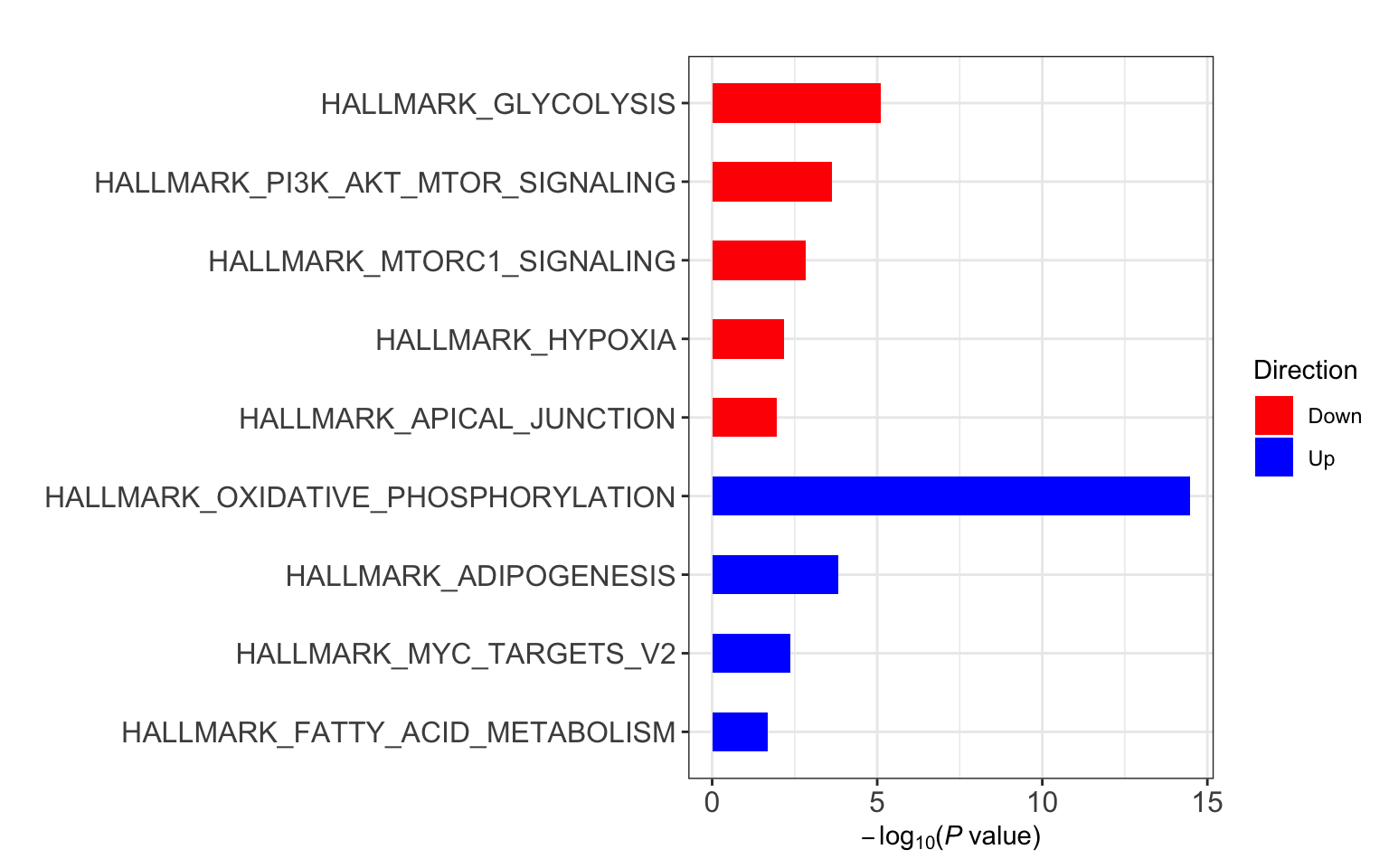
C6
res <- runCamera(proMat, designMat, gmts$C6, id = rowData(protCLL[rownames(proMat),])$hgnc_symbol)
res$enrichPlot
Annotate PC2
Correlation test
Assocation test
proMat <- assays(protCLL)[["QRILC"]]
pc <- pcRes[,2][colnames(proMat)]
designMat <- model.matrix(~1+pc)
fit <- lmFit(proMat,  designMat)
fit2 <- eBayes(fit)
corRes.pc2 <- topTable(fit2, number ="all", adjust.method = "BH", coef = "pc") %>% rownames_to_column("id") %>%
    mutate(symbol = rowData(protCLL[id,])$hgnc_symbol)
Number of significant associations (10% FDR)
hist(corRes.pc2$P.Value,breaks=100)
Table of significant associations (5% FDR)
resTab.sig <- filter(corRes.pc2, adj.P.Val < 0.05) %>%
  select(symbol, id,logFC, P.Value, adj.P.Val) %>%
  arrange(P.Value)
resTab.sig %>% mutate_if(is.numeric, formatC, digits=2, format= "e") %>%
  DT::datatable()
Heatmap of associated genes
colAnno <- tibble(patID = colnames(proMat), PC2 = pcRes[colnames(proMat),2]) %>%
  arrange(PC2) %>% data.frame() %>% column_to_rownames("patID")

plotMat <- proMat[resTab.sig$id[1:100],rownames(colAnno)]
plotMat <- jyluMisc::mscale(plotMat, censor = 6)

pheatmap(plotMat, scale = "none", annotation_col = colAnno, clustering_method = "ward.D2",
         cluster_cols = FALSE,
         labels_row = resTab.sig$symbol[1:100], color = colorRampPalette(c("navy","white","firebrick"))(100),
         breaks = seq(-6,6, length.out = 101))
Enrichment using Camera
res <- runCamera(proMat, designMat, gmts$H, id = rowData(protCLL[rownames(proMat),])$hgnc_symbol)
res$enrichPlot
Compare this batch with the previous LUMOS data
Prepare combined datasets
load("../../var/proteomic_newLUMOS_20201124.RData")
protNew <- protCLL_raw
protNew$patID <- colnames(protNew)
protNew$batch <- "new"
colnames(protNew) <- paste0(protNew$patID,seq(ncol(protNew)))

load("../../var/proteomic_LUMOS_20200430.RData")
protOld <- protCLL_raw
protOld$patID <- colnames(protOld)
protOld$batch <- "old"
colnames(protOld) <- paste0(protOld$patID,seq(ncol(protOld)))

overGene <- na.omit(intersect(rowData(protNew)$ensembl_gene_id, rowData(protOld)$ensembl_gene_id))
length(overGene)
[1] 3345protNew <- protNew[match(overGene, rowData(protNew)$ensembl_gene_id),]
rownames(protNew) <- rowData(protNew)$ensembl_gene_id
protOld <- protOld[match(overGene, rowData(protOld)$ensembl_gene_id),]
rownames(protOld) <- rowData(protOld)$ensembl_gene_id
countMat <- cbind(assays(protOld)[["count"]],assays(protNew)[["count"]])
#remove proteins with more than 50% missing values
missPer <- apply(countMat,1,function(x) sum(is.na(x)/ncol(countMat)))
countMat <- countMat[missPer <= 0.5,]
#prepare sampel annotations
patAnno <- rbind(colData(protOld)[,c("patID","sampleID","batch")], colData(protNew)[,c("patID","sampleID","batch")])
protCom <- SummarizedExperiment(assays = list(count = countMat), colData = patAnno)
#assign protein annotations
rowData(protCom) <- rowData(protOld[rownames(protCom),])Perform normalization on combined matrix
resVsn <- vsn::vsn2(countMat)
exprMat <- vsn::predict(resVsn, countMat)
assays(protCom)[["expr"]] <- exprMat
Check the distribution after normalization
protTab <- jyluMisc::sumToTiday(protCom)
ggplot(protTab, aes(x=patID, y=expr, fill = batch)) + geom_boxplot() +
  theme_bw() + theme(axis.text.x = element_text(angle = 90, hjust=1, vjust = .5))
Looks fine
Imputation
protImp <- protCom
rowData(protImp)$ID <- rowData(protImp)$name
assays(protImp)[["count"]] <- NULL
protImp <- DEP::impute(protImp, fun = "QRILC")
assays(protCom)[["QRILC"]] <- assays(protImp)[["expr"]]
PCA
exprMat <- assays(protCom)[["QRILC"]]
pcRes <- prcomp(t(exprMat), center =TRUE, scale. = FALSE)$x
plotTab <- pcRes[,1:2] %>% data.frame() %>% rownames_to_column("id") %>%
  mutate(batch = patAnno[id,]$batch,
         patID = patAnno[id,]$patID)
ggplot(plotTab, aes(x=PC1, y=PC2, col = batch)) +
  geom_text(aes(label = patID)) + theme_bw()
Two batchs are separated.
PC1 separates batches. PC2 pontentially captures the variance related to viability after sorting.
Heatmap and hierarchical clustering
exprMat <- assays(protCom)[["expr"]]
sds <- rowSds(exprMat, na.rm = TRUE)
exprMat <- exprMat[order(sds, decreasing = TRUE)[1:1000],]
exprMat <- jyluMisc::mscale(exprMat, censor = 5)
colAnno <- data.frame(row.names = colnames(exprMat), batch = protCom$batch)
pheatmap(exprMat, scale="none", annotation_col = colAnno, clustering_method = "ward.D2",
         labels_row = rowData(protCom[rownames(exprMat),])$hgnc_symbol)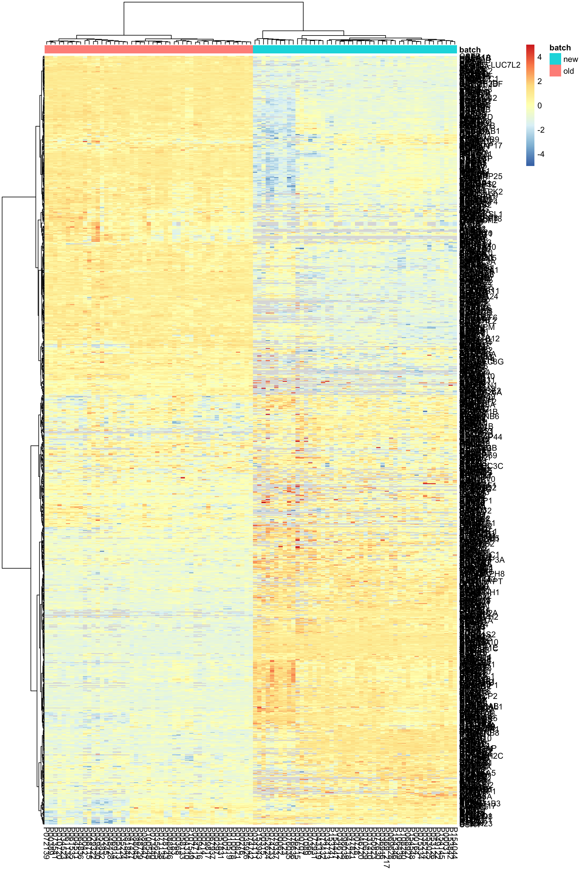
Check the reproduciblity of the samples present in both batches.
dupPat <- intersect(protNew$patID, protOld$patID)
plotTab <- protTab %>% filter(patID %in% dupPat) %>%
  select(rowID, expr, patID, batch) %>%
  pivot_wider(names_from = batch, values_from = expr)
ggplot(plotTab, aes(x=old, y=new)) + geom_point() + geom_smooth(method ="lm", se = FALSE) +
  facet_wrap(~patID)
Overall looks fine
Can the batch effect be removed?
Remove batch effect using Limma
exprMat <- assays(protCom)[["expr"]]
exprMat.re <- limma::removeBatchEffect(exprMat, batch = factor(protCom$batch))
assays(protCom)[["fix"]] <- exprMat.re
Imputation
protImp <- protCom
rowData(protImp)$ID <- rowData(protImp)$name
assays(protImp)[["count"]] <- NULL
assays(protImp)[["expr"]] <- NULL
assays(protImp)[["QRILC"]] <- NULL
protImp <- DEP::impute(protImp, fun = "QRILC")
assays(protCom)[["QRILC_fix"]] <- assays(protImp)[["fix"]]
PCA
exprMat <- assays(protCom)[["QRILC_fix"]]
#sds <- rowSds(exprMat, na.rm = TRUE)
#exprMat <- exprMat[order(sds, decreasing = TRUE)[1:2000],]
pcRes <- prcomp(t(exprMat), center =TRUE, scale. = FALSE)$x
plotTab <- pcRes[,1:2] %>% data.frame() %>% rownames_to_column("id") %>%
mutate(batch = patAnno[id,]$batch,
patID = patAnno[id,]$patID)
ggplot(plotTab, aes(x=PC1, y=PC2, col = batch)) +
geom_text(aes(label = patID)) + theme_bw()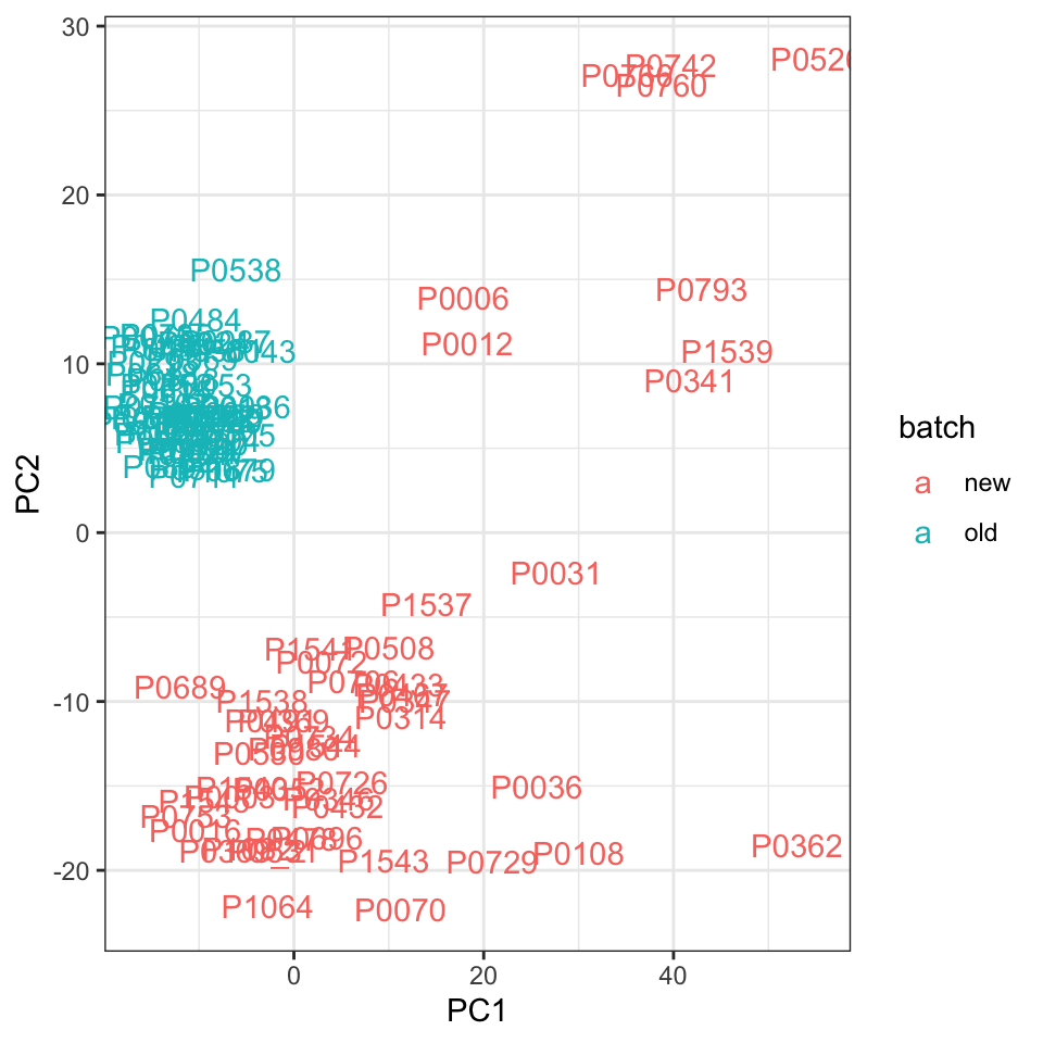 Batches are not separated by PC1, but can still be separated by higher dimensions.
Heatmap and hierarchical clustering
exprMat <- assays(protCom)[["fix"]]
sds <- rowSds(exprMat, na.rm = TRUE)
exprMat <- exprMat[order(sds, decreasing = TRUE)[1:1000],]
exprMat <- jyluMisc::mscale(exprMat, censor = 5)
colAnno <- data.frame(row.names = colnames(exprMat), batch = protCom$batch)
pheatmap(exprMat, scale="none", annotation_col = colAnno, clustering_method = "ward.D2",
         labels_row = rowData(protCom[rownames(exprMat),])$hgnc_symbol)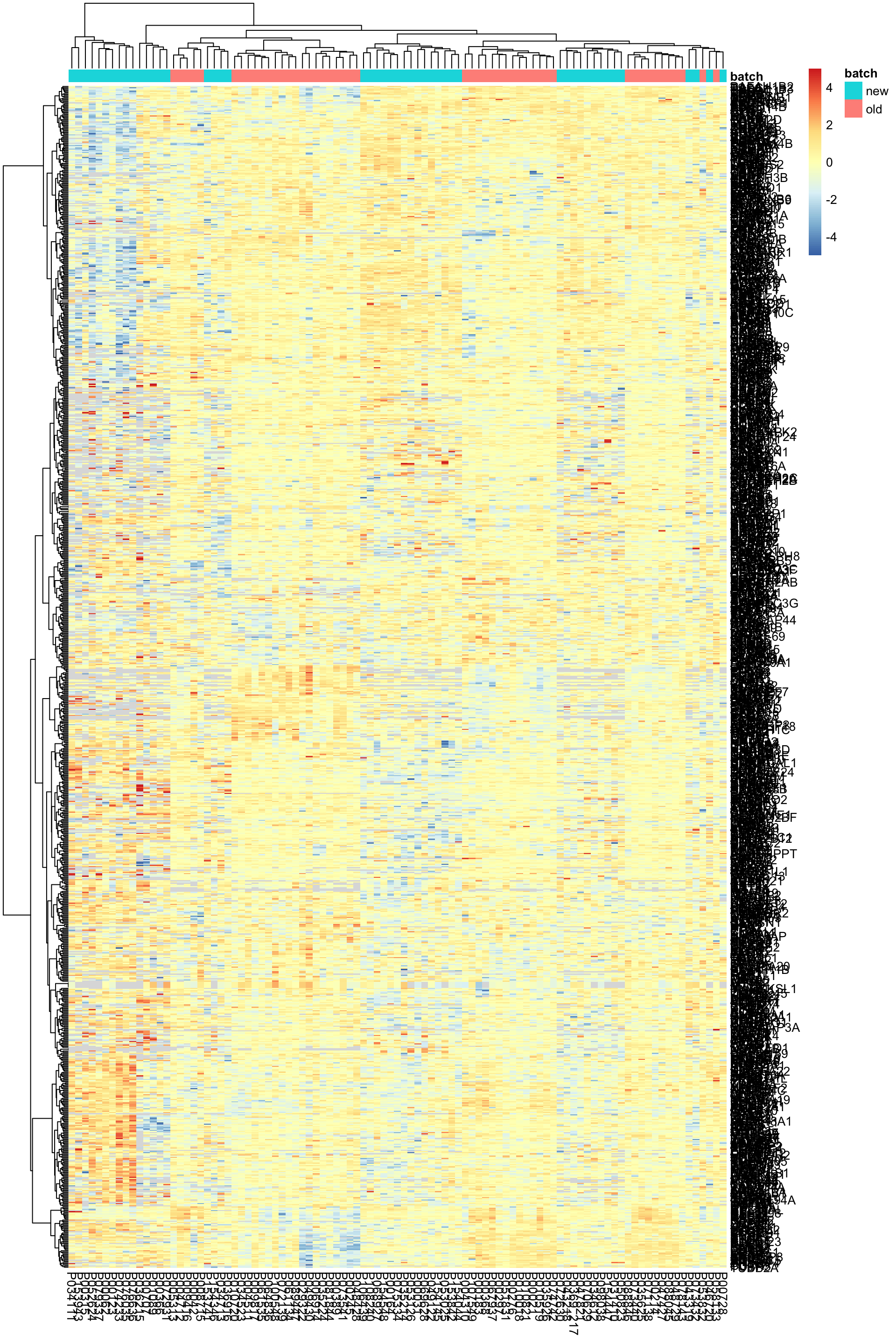
Check the reproduciblity of the samples present in both batches.
protTab <- jyluMisc::sumToTiday(protCom)
dupPat <- intersect(protNew$patID, protOld$patID)
plotTab <- protTab %>% filter(patID %in% dupPat) %>%
select(rowID, fix, patID, batch) %>%
pivot_wider(names_from = batch, values_from = fix)
ggplot(plotTab, aes(x=old, y=new)) + geom_point() + geom_smooth(method ="lm", se = FALSE) +
facet_wrap(~patID)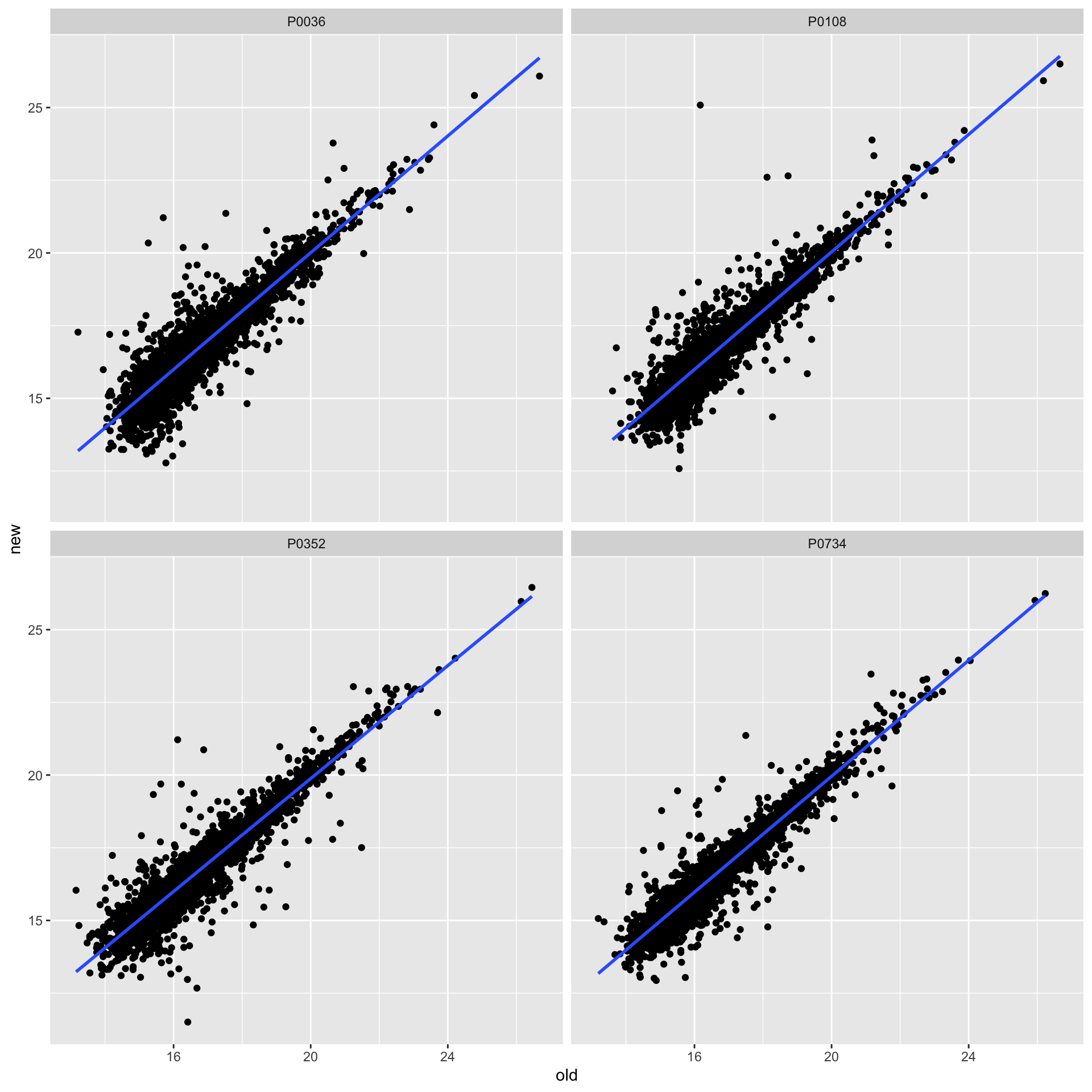 Looks better than without fixing.
Save the post process object
#assays(protCLL)[["QRILC_re"]] <- protMat.new
#protCLL$PC1 <- pcRes[colnames(protCLL),1]
#protCLL$PC2 <- pcRes[colnames(protCLL),2]
#save(protCLL, file = "../output/LUMOSnew_processed.RData")
sessionInfo()R version 3.6.0 (2019-04-26)
Platform: x86_64-apple-darwin15.6.0 (64-bit)
Running under: macOS 10.15.7
Matrix products: default
BLAS: /Library/Frameworks/R.framework/Versions/3.6/Resources/lib/libRblas.0.dylib
LAPACK: /Library/Frameworks/R.framework/Versions/3.6/Resources/lib/libRlapack.dylib
locale:
[1] en_US.UTF-8/en_US.UTF-8/en_US.UTF-8/C/en_US.UTF-8/en_US.UTF-8
attached base packages:
[1] parallel stats4 stats graphics grDevices utils datasets
[8] methods base
other attached packages:
[1] forcats_0.5.0 stringr_1.4.0
[3] dplyr_1.0.0 purrr_0.3.4
[5] readr_1.3.1 tidyr_1.1.0
[7] tibble_3.0.3 ggplot2_3.3.2
[9] tidyverse_1.3.0 DESeq2_1.26.0
[11] SummarizedExperiment_1.16.1 DelayedArray_0.12.3
[13] BiocParallel_1.20.1 matrixStats_0.56.0
[15] Biobase_2.46.0 GenomicRanges_1.38.0
[17] GenomeInfoDb_1.22.1 IRanges_2.20.2
[19] S4Vectors_0.24.4 BiocGenerics_0.32.0
[21] jyluMisc_0.1.5 pheatmap_1.0.12
[23] piano_2.2.0 cowplot_1.0.0
[25] limma_3.42.2
loaded via a namespace (and not attached):
[1] DEP_1.8.0 utf8_1.1.4 shinydashboard_0.7.1
[4] gmm_1.6-5 tidyselect_1.1.0 RSQLite_2.2.0
[7] AnnotationDbi_1.48.0 htmlwidgets_1.5.1 grid_3.6.0
[10] norm_1.0-9.5 maxstat_0.7-25 munsell_0.5.0
[13] preprocessCore_1.48.0 codetools_0.2-16 DT_0.14
[16] withr_2.2.0 colorspace_1.4-1 knitr_1.29
[19] rstudioapi_0.11 ggsignif_0.6.0 mzID_1.24.0
[22] labeling_0.3 git2r_0.27.1 slam_0.1-47
[25] GenomeInfoDbData_1.2.2 KMsurv_0.1-5 bit64_0.9-7
[28] farver_2.0.3 rprojroot_1.3-2 vctrs_0.3.1
[31] generics_0.0.2 TH.data_1.0-10 xfun_0.15
[34] sets_1.0-18 doParallel_1.0.15 R6_2.4.1
[37] clue_0.3-57 locfit_1.5-9.4 bitops_1.0-6
[40] fgsea_1.12.0 assertthat_0.2.1 promises_1.1.1
[43] scales_1.1.1 multcomp_1.4-13 nnet_7.3-14
[46] gtable_0.3.0 affy_1.64.0 sandwich_2.5-1
[49] workflowr_1.6.2 rlang_0.4.7 genefilter_1.68.0
[52] mzR_2.20.0 GlobalOptions_0.1.2 splines_3.6.0
[55] rstatix_0.6.0 impute_1.60.0 acepack_1.4.1
[58] broom_0.7.0 checkmate_2.0.0 BiocManager_1.30.10
[61] yaml_2.2.1 abind_1.4-5 modelr_0.1.8
[64] crosstalk_1.1.0.1 backports_1.1.8 httpuv_1.5.4
[67] Hmisc_4.4-0 tools_3.6.0 relations_0.6-9
[70] affyio_1.56.0 ellipsis_0.3.1 gplots_3.0.4
[73] RColorBrewer_1.1-2 MSnbase_2.12.0 plyr_1.8.6
[76] Rcpp_1.0.5 base64enc_0.1-3 visNetwork_2.0.9
[79] zlibbioc_1.32.0 RCurl_1.98-1.2 ggpubr_0.4.0
[82] rpart_4.1-15 GetoptLong_1.0.2 zoo_1.8-8
[85] haven_2.3.1 ggrepel_0.8.2 cluster_2.1.0
[88] exactRankTests_0.8-31 fs_1.4.2 magrittr_1.5
[91] data.table_1.12.8 openxlsx_4.1.5 circlize_0.4.10
[94] reprex_0.3.0 survminer_0.4.7 pcaMethods_1.78.0
[97] mvtnorm_1.1-1 ProtGenerics_1.18.0 hms_0.5.3
[100] shinyjs_1.1 mime_0.9 evaluate_0.14
[103] xtable_1.8-4 XML_3.98-1.20 rio_0.5.16
[106] jpeg_0.1-8.1 readxl_1.3.1 shape_1.4.4
[109] gridExtra_2.3 compiler_3.6.0 ncdf4_1.17
[112] KernSmooth_2.23-17 crayon_1.3.4 htmltools_0.5.0
[115] mgcv_1.8-31 later_1.1.0.1 Formula_1.2-3
[118] geneplotter_1.64.0 lubridate_1.7.9 DBI_1.1.0
[121] ComplexHeatmap_2.2.0 dbplyr_1.4.4 tmvtnorm_1.4-10
[124] MASS_7.3-51.6 Matrix_1.2-18 car_3.0-8
[127] cli_2.0.2 imputeLCMD_2.0 vsn_3.54.0
[130] marray_1.64.0 gdata_2.18.0 igraph_1.2.5
[133] pkgconfig_2.0.3 km.ci_0.5-2 foreign_0.8-71
[136] foreach_1.5.0 MALDIquant_1.19.3 xml2_1.3.2
[139] annotate_1.64.0 XVector_0.26.0 drc_3.0-1
[142] rvest_0.3.5 digest_0.6.25 rmarkdown_2.3
[145] cellranger_1.1.0 fastmatch_1.1-0 survMisc_0.5.5
[148] htmlTable_2.0.1 curl_4.3 shiny_1.5.0
[151] gtools_3.8.2 rjson_0.2.20 lifecycle_0.2.0
[154] nlme_3.1-148 jsonlite_1.7.0 carData_3.0-4
[157] fansi_0.4.1 pillar_1.4.6 lattice_0.20-41
[160] fastmap_1.0.1 httr_1.4.1 plotrix_3.7-8
[163] survival_3.2-3 glue_1.4.1 zip_2.0.4
[166] iterators_1.0.12 png_0.1-7 bit_4.0.4
[169] stringi_1.4.6 blob_1.2.1 latticeExtra_0.6-29
[172] caTools_1.18.0 memoise_1.1.0