Integrative analysis using MOFA
Junyan Lu
2022-05-04
Last updated: 2024-04-08
Checks: 5 1
Knit directory: RA_Tcell_omics/analysis/
This reproducible R Markdown analysis was created with workflowr (version 1.7.0). The Checks tab describes the reproducibility checks that were applied when the results were created. The Past versions tab lists the development history.
Great job! The global environment was empty. Objects defined in the global environment can affect the analysis in your R Markdown file in unknown ways. For reproduciblity it’s best to always run the code in an empty environment.
The command set.seed(20221110) was run prior to running
the code in the R Markdown file. Setting a seed ensures that any results
that rely on randomness, e.g. subsampling or permutations, are
reproducible.
Great job! Recording the operating system, R version, and package versions is critical for reproducibility.
Nice! There were no cached chunks for this analysis, so you can be confident that you successfully produced the results during this run.
Great job! Using relative paths to the files within your workflowr project makes it easier to run your code on other machines.
Tracking code development and connecting the code version to the
results is critical for reproducibility. To start using Git, open the
Terminal and type git init in your project directory.
This project is not being versioned with Git. To obtain the full
reproducibility benefits of using workflowr, please see
?wflow_start.
Load libraries
Load and process data
load("../output/maeObj.RData")Metabolomics
seMeta <- maeObj[["Metabolism"]]
#seMata <- seMeta[,!is.na(seMeta$dateMeta)]
#metaMat <- assay(seMata)
#metaMat <- glog(metaMat)
#metaMat <- sva::ComBat(metaMat, batch = seMata$dateMeta)


#glog transformation
metaMat <- glog(assay(seMeta))

#center and scale
#metaMat <- jyluMisc::mscale(metaMat)
Proteome (use the new DIA proteomic)
seProt <- maeObj[["Proteome_DIA"]]
sds <- genefilter::rowSds(assays(seProt)[["norm"]],na.rm=TRUE)
seProt <- seProt[order(sds, decreasing = T),]
seProt <- seProt[!duplicated(rowData(seProt)$symbol),]

protMat <- assays(seProt)[["norm"]]
rownames(protMat) <- rowData(seProt)$symbol
Phosphoproteome
sePhos <- maeObj[["Phosphoproteome"]]
sePhos <- sePhos[!rowData(sePhos)$site %in% c("",NA),]
sds <- genefilter::rowSds(assays(sePhos)[["norm"]],na.rm=TRUE)
sePhos <- sePhos[order(sds, decreasing = T),]
sePhos <- sePhos[!duplicated(rowData(sePhos)$site),]

phosMat <- assays(sePhos)[["norm"]]
rownames(phosMat) <- rowData(sePhos)$site
Phosphoproteome normalized by protein expression
seRatio <- maeObj[["PhosRatio"]]
seRatio <- seRatio[!rowData(seRatio)$site %in% c("",NA),]
sds <- genefilter::rowSds(assay(seRatio),na.rm=TRUE)
seRatio <- seRatio[order(sds, decreasing = T),]
seRatio <- seRatio[!duplicated(rowData(seRatio)$site),]

ratioMat <- assay(seRatio)
rownames(ratioMat) <- rowData(seRatio)$site
Methylation
methMat <- assay(maeObj[["Methylation"]])FACS
facsMat <- assay(maeObj[["FACS"]])
facsMat  <- vsn::justvsn(facsMat)
rownames(facsMat) <- rowData(maeObj[["FACS"]])$feature
Create MAE object for mofa
mofaMae <- MultiAssayExperiment(experiments = list(meta = metaMat, prot = protMat, phos = phosMat, meth = methMat, FACS = facsMat),
                                colData = colData(maeObj))
Only keep samples that have at least four assays
useSamples <- MultiAssayExperiment::sampleMap(mofaMae) %>%
  as_tibble() %>% group_by(primary) %>% summarise(n= length(assay)) %>%
  filter(n >= 2) %>% pull(primary)
mofaMae <- mofaMae[,useSamples]
MOFAobject <- create_mofa_from_MultiAssayExperiment(mofaMae)Plot data overview
plot_data_overview(MOFAobject)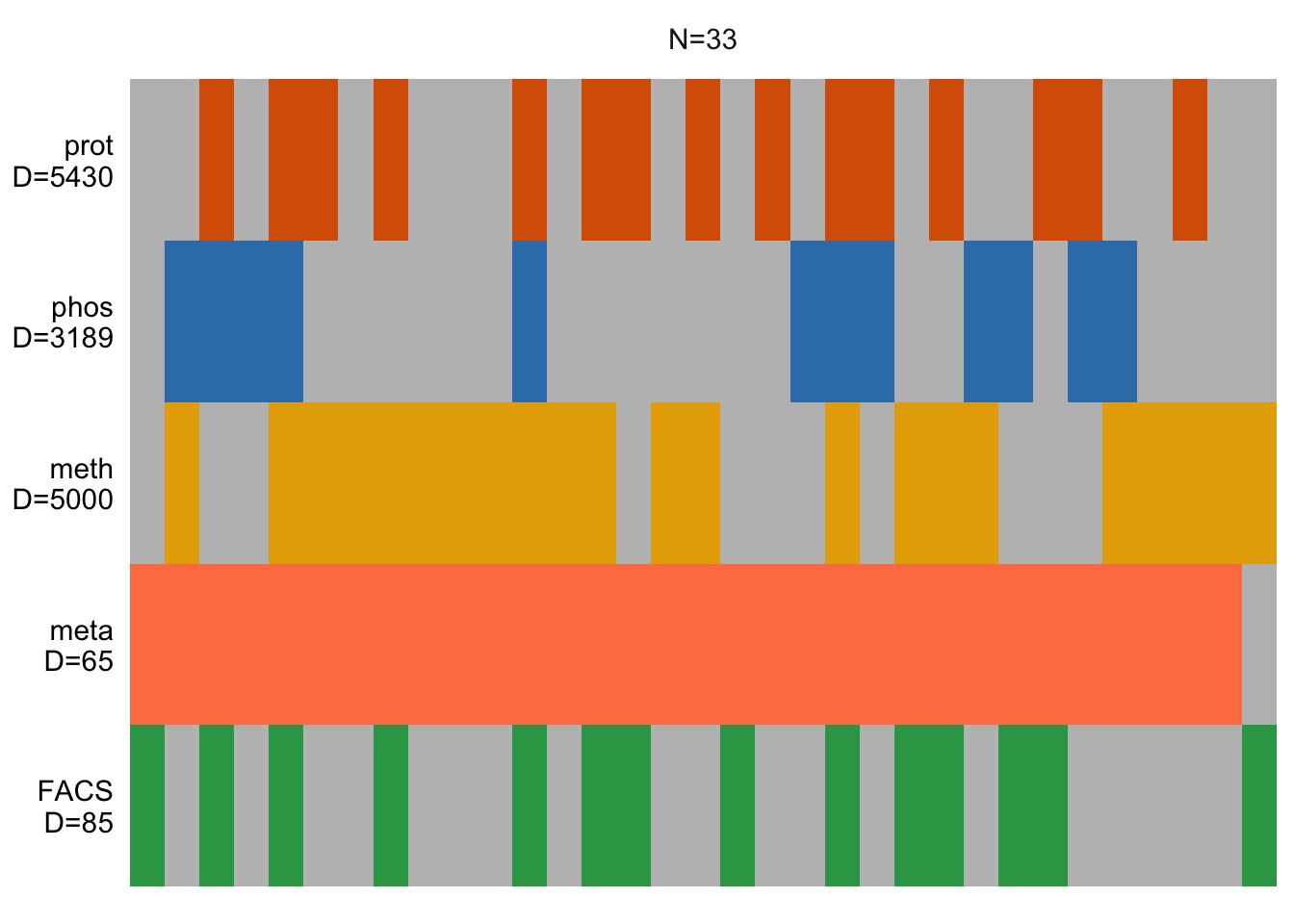
Define MOFA options
Data options
data_opts <- get_default_data_options(MOFAobject)
data_opts
$scale_views
[1] FALSE
$scale_groups
[1] FALSE
$center_groups
[1] TRUE
$use_float32
[1] FALSE
$views
[1] "meta" "prot" "phos" "meth" "FACS"
$groups
[1] "group1"Model options
model_opts <- get_default_model_options(MOFAobject)
#model_opts$spikeslab_weights <- FALSE

model_opts$num_factors <- 10
model_opts
$likelihoods
meta prot phos meth FACS
"gaussian" "gaussian" "gaussian" "gaussian" "gaussian"
$num_factors
[1] 10
$spikeslab_factors
[1] FALSE
$spikeslab_weights
[1] TRUE
$ard_factors
[1] FALSE
$ard_weights
[1] TRUETraining options
train_opts <- get_default_training_options(MOFAobject)
train_opts$convergence_mode <- "slow"
train_opts$seed <- 2022
train_opts$maxiter <- 10000
train_opts
$maxiter
[1] 10000
$convergence_mode
[1] "slow"
$drop_factor_threshold
[1] -1
$verbose
[1] FALSE
$startELBO
[1] 1
$freqELBO
[1] 5
$stochastic
[1] FALSE
$gpu_mode
[1] FALSE
$seed
[1] 2022
$outfile
NULL
$weight_views
[1] FALSE
$save_interrupted
[1] FALSEChange drop threshold to 0.01
train_opts$drop_factor_threshold <-0.01Train the MOFA model
Prepare MOFA object
MOFAobject <- prepare_mofa(MOFAobject,
  data_options = data_opts,
  model_options = model_opts,
  training_options = train_opts
)
Add usefull metadata
sampleTab <- colData(mofaMae) %>% data.frame() %>% rownames_to_column("sample") %>% dplyr::rename(phenotype = group)
samples_metadata(MOFAobject) <- sampleTab
Training
MOFAobject <- run_mofa(MOFAobject)
saveRDS(MOFAobject,"../output/mofaOut.rds")
Preliminary analysis of the results
MOFAobject <- readRDS("../output/mofaOut.rds")Factor correlation matrix
plot_factor_cor(MOFAobject)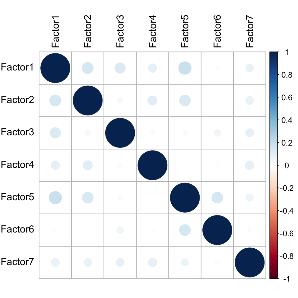
Variance explained
plot_variance_explained(MOFAobject, max_r2=15)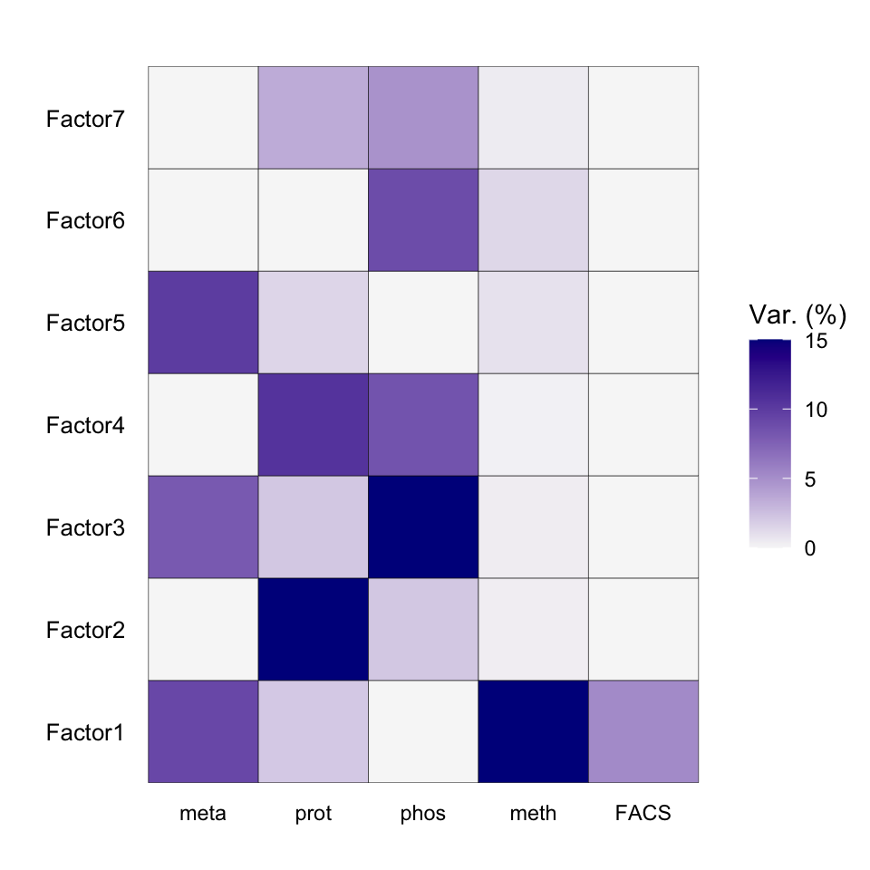
Total variance explained
plot_variance_explained(MOFAobject, plot_total = T)[[2]]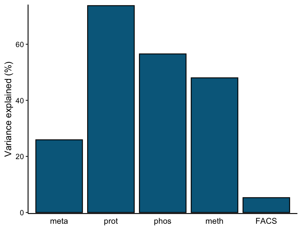
correlate_factors_with_covariates(MOFAobject,
  plot="log_pval",
  covariates = c("Gender","phenotype", "Age","CCP","GC","Leflunomid","MTX", "Quensyl","RF","Sulfasalazin","CRP","DAS28"))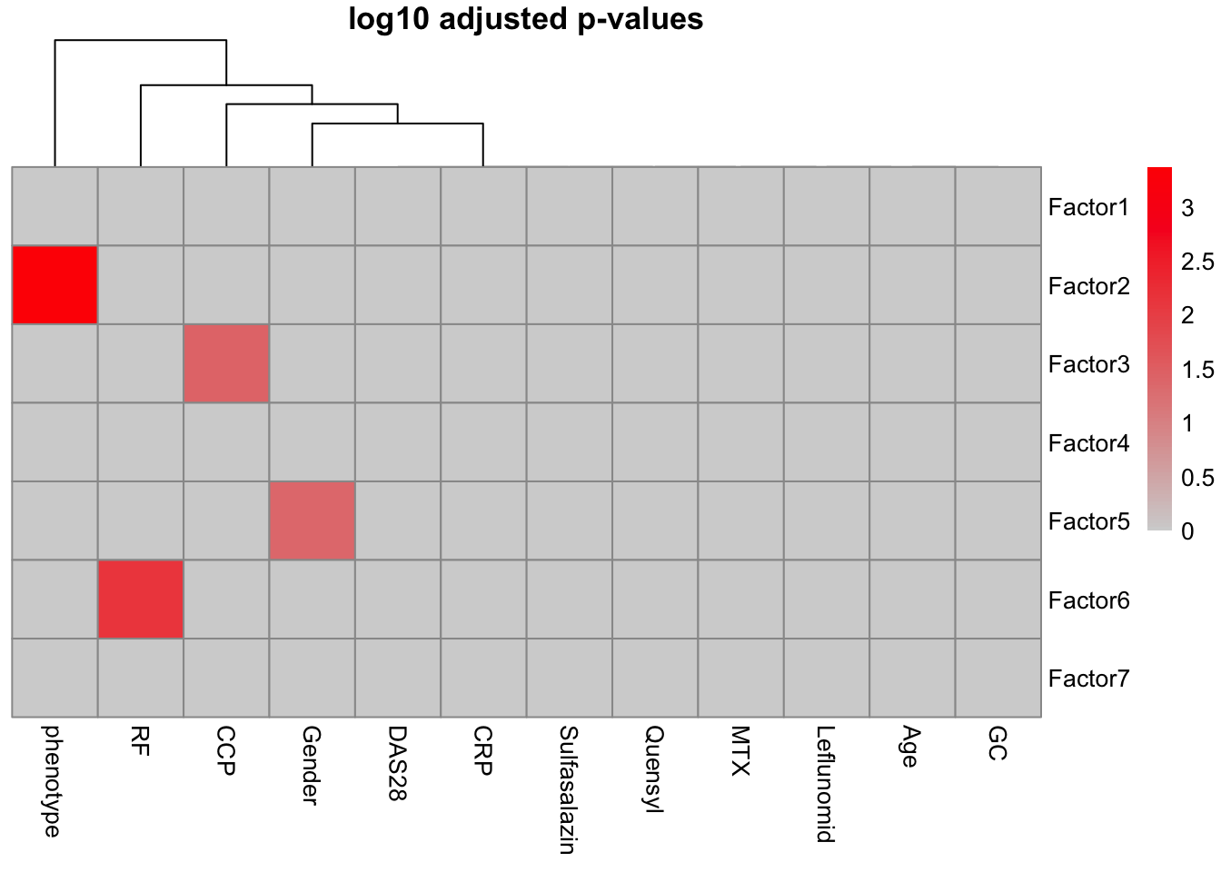
T-test
facTab <- get_factors(MOFAobject, groups = "group1", as.data.frame = TRUE) %>%
    mutate(phenotype = colData(mofaMae)[sample,]$group)

resTab <- facTab %>% group_by(factor) %>% nest() %>%
    mutate(m=map(data, ~t.test(value~phenotype, data=., var.equal=TRUE))) %>%
    mutate(res = map(m, broom::tidy)) %>%
    unnest(res) %>%
    select(factor, estimate, p.value)
resTab
# A tibble: 7 × 3
# Groups: factor [7]
factor estimate p.value
<fct> <dbl> <dbl>
1 Factor1 -0.516 0.506
2 Factor2 1.23 0.000428
3 Factor3 0.572 0.0975
4 Factor4 0.204 0.388
5 Factor5 0.340 0.291
6 Factor6 -0.135 0.506
7 Factor7 -0.406 0.214 plotTab <- select(facTab, factor, sample, value, phenotype) %>%
filter(factor %in% c("Factor1","Factor2")) %>%
pivot_wider(names_from = factor, values_from = value)
ggplot(plotTab, aes(x=Factor1, y=Factor2, color = phenotype)) +
geom_point() +
ggrepel::geom_text_repel(aes(label = sample)) +
theme_bw()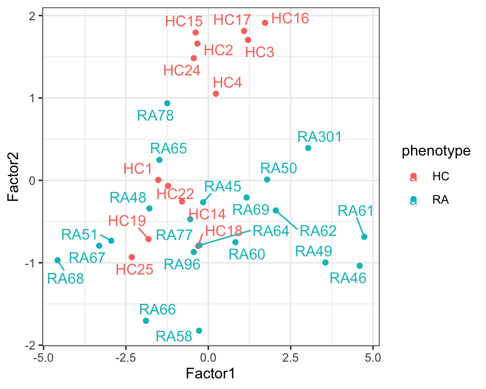
Focus on F1
Weight of proteomics features
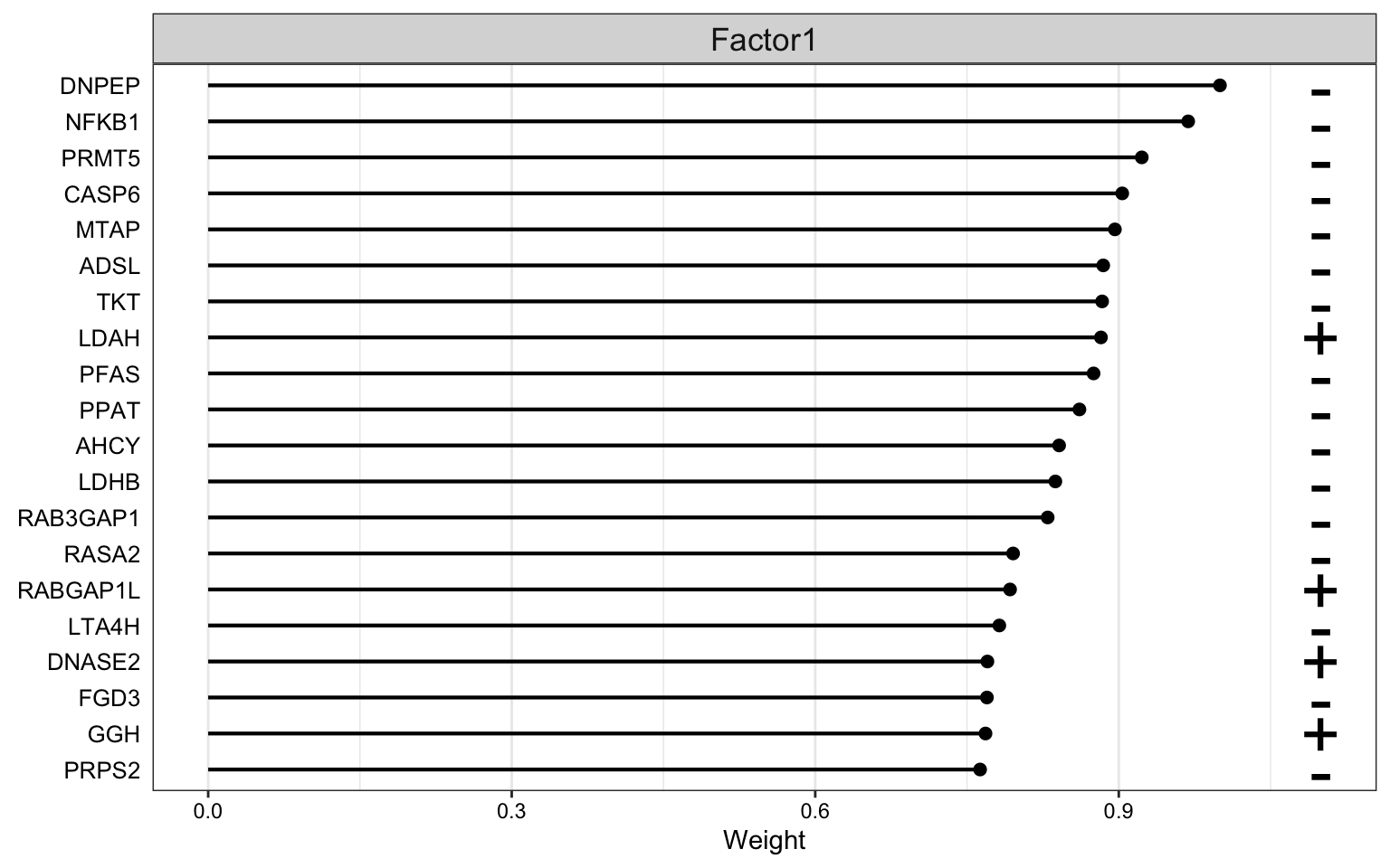
plot_top_weights(MOFAobject,
 view = "prot",
 factor = 1,
 nfeatures = 20,     # Top number of features to highlight
 scale = T           # Scale weights from -1 to 1
)
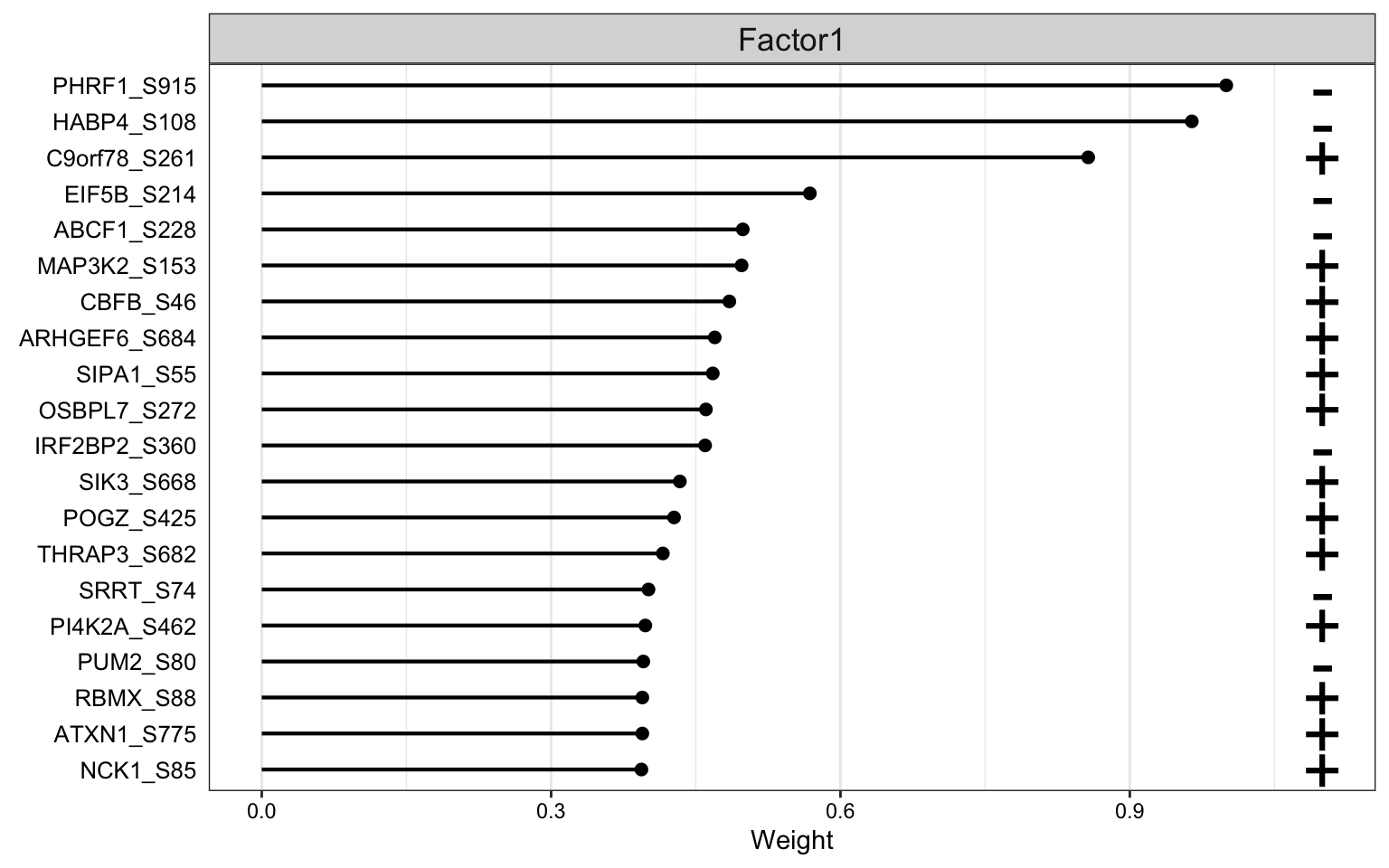
Weight of phosphoproteomic features
plot_top_weights(MOFAobject,
 view = "phos",
 factor = 1,
 nfeatures = 20,     # Top number of features to highlight
 scale = T           # Scale weights from -1 to 1
)
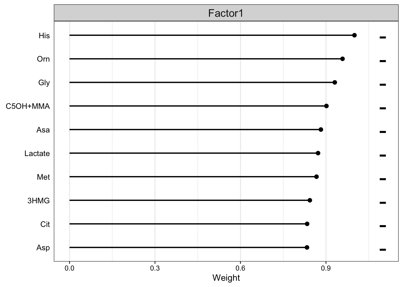
Weight of metabolic features
plot_top_weights(MOFAobject,
 view = "meta",
 factor = 1,
 nfeatures = 10,     # Top number of features to highlight
 scale = T           # Scale weights from -1 to 1
)
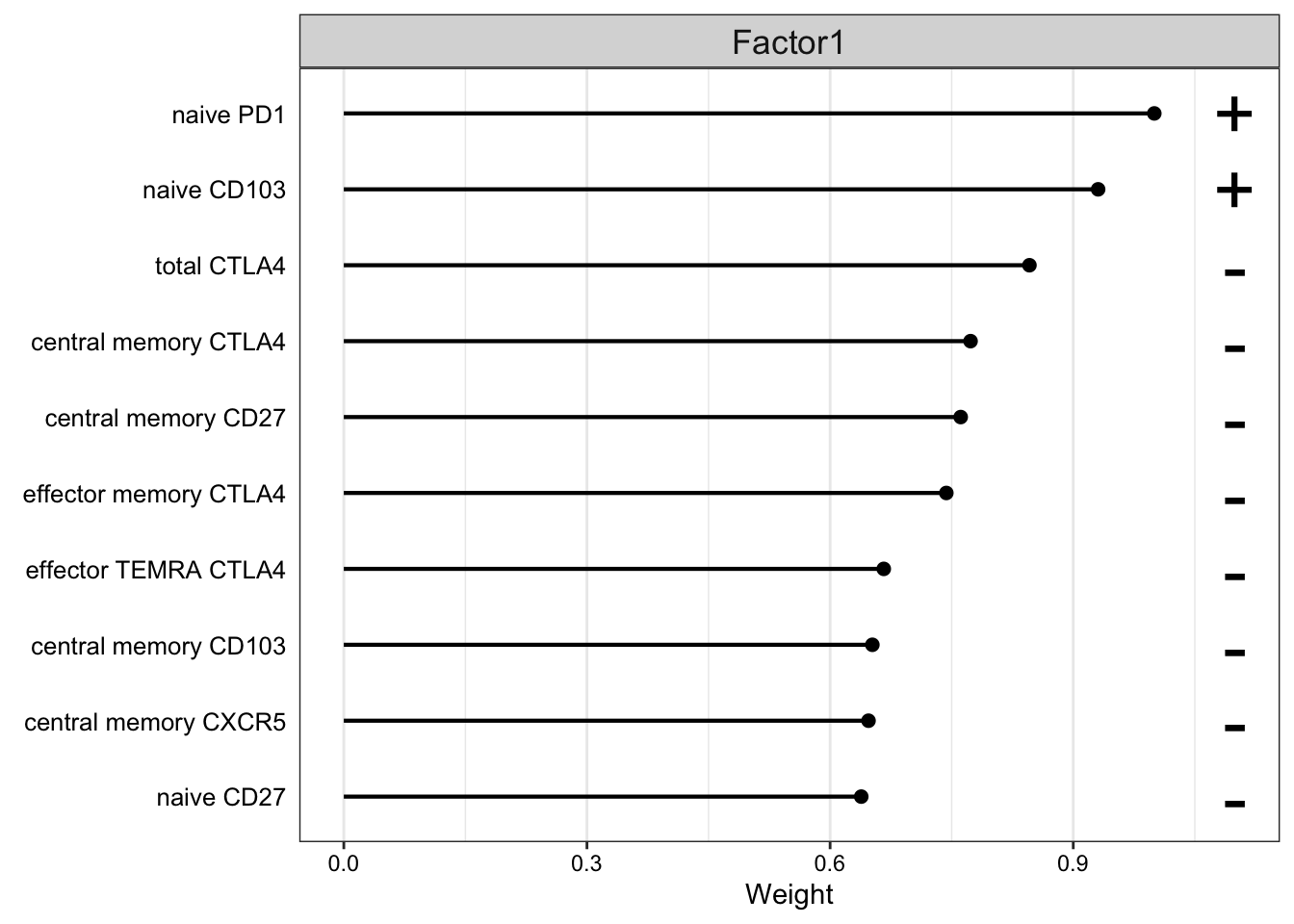
Weight of FACS features
plot_top_weights(MOFAobject,
 view = "FACS",
 factor = 1,
 nfeatures = 10,     # Top number of features to highlight
 scale = T           # Scale weights from -1 to 1
)
Focus on F2
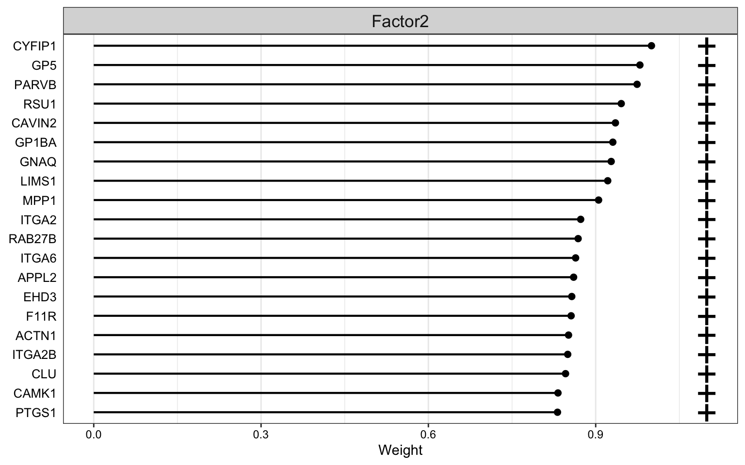
Weight of proteomics features
plot_top_weights(MOFAobject,
 view = "prot",
 factor = 2,
 nfeatures = 20,     # Top number of features to highlight
 scale = T           # Scale weights from -1 to 1
)
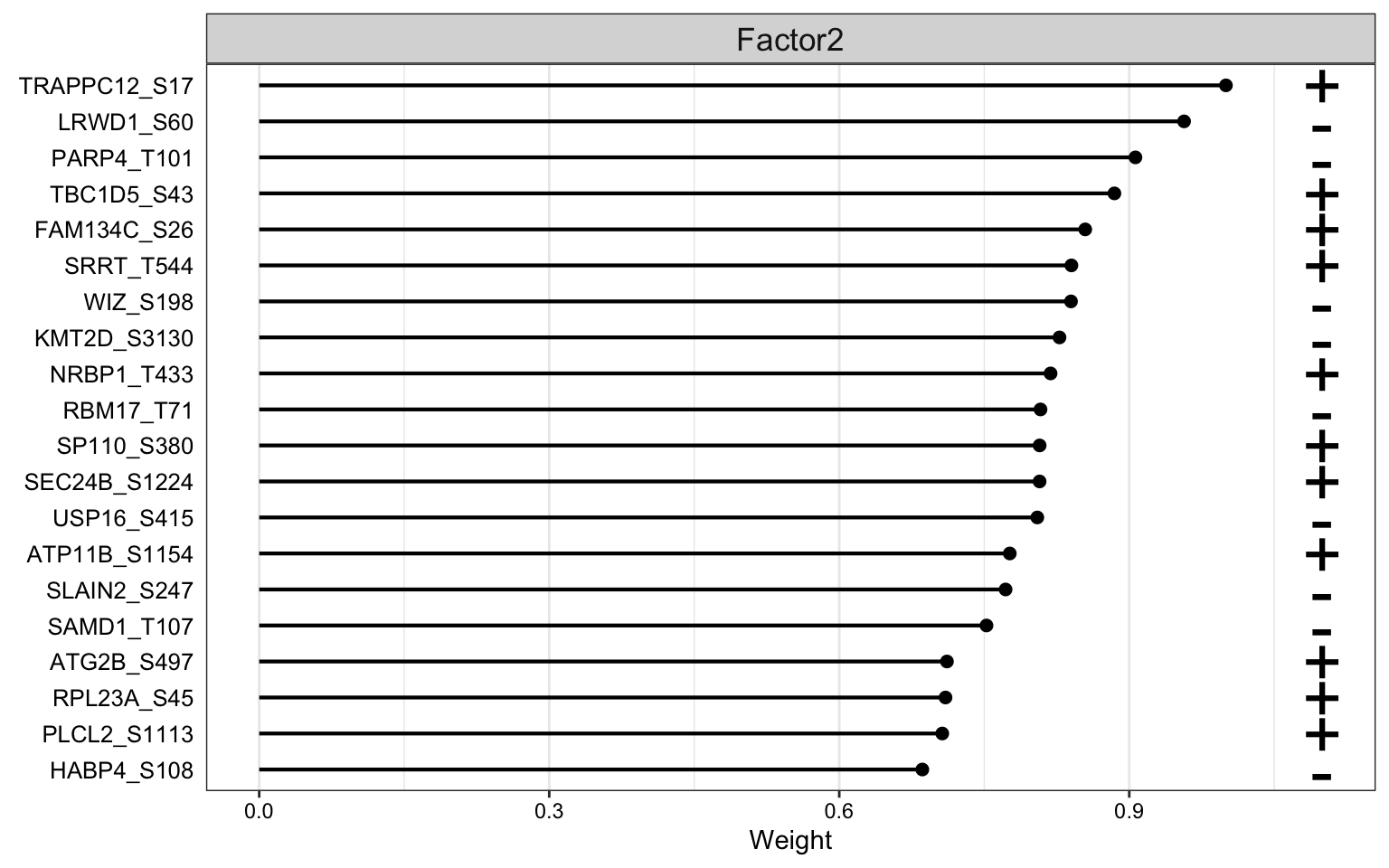
Weight of phosphoproteomic features
plot_top_weights(MOFAobject,
 view = "phos",
 factor = 2,
 nfeatures = 20,     # Top number of features to highlight
 scale = T           # Scale weights from -1 to 1
)
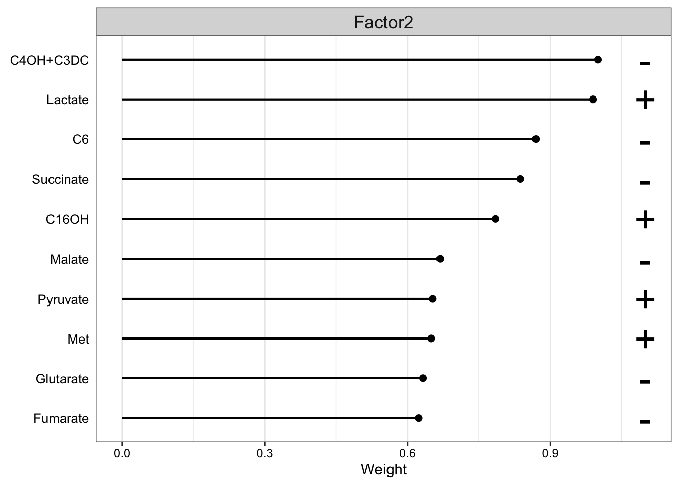
Weight of metabolic features
plot_top_weights(MOFAobject,
 view = "meta",
 factor = 2,
 nfeatures = 10,     # Top number of features to highlight
 scale = T           # Scale weights from -1 to 1
)
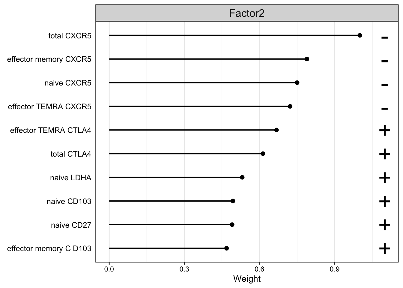
Weight of FACS features
plot_top_weights(MOFAobject,
 view = "FACS",
 factor = 2,
 nfeatures = 10,     # Top number of features to highlight
 scale = T           # Scale weights from -1 to 1
)
Enrichment
gmts <- list(H = "~/CLLproject_jlu/data/commonFiles/h.all.v6.2.symbols.gmt",
             KEGG = "~/CLLproject_jlu/data/commonFiles/c2.cp.kegg.v6.2.symbols.gmt",
             GOBP = "~/CLLproject_jlu/data/commonFiles/c5.bp.v6.2.symbols.gmt",
             C6 = "~/CLLproject_jlu/data/commonFiles/c6.all.v6.2.symbols.gmt")

listToMat <- function(gmts) {
    allMat <- lapply(names(gmts), function(gmtName) {
        gsc <- piano::loadGSC(gmts[[gmtName]])$gsc
        sigMat <- lapply(names(gsc), function(setName) {
            tibble(set = setName, feature = gsc[[setName]])
        }) %>% bind_rows() %>%
            mutate(val = 1) %>%
            pivot_wider(names_from = feature, values_from = val) %>%
            column_to_rownames("set") %>% as.matrix()

        sigMat[is.na(sigMat)] <- 0
        sigMat
    })
    names(allMat) <- names(gmts)
    return(allMat)
}

sigMat <- listToMat(gmts)
enRes.H <- run_enrichment(MOFAobject, view = "prot", factors = c(1,2), feature.sets = sigMat$H, set.statistic = "mean.diff",
sign = "all", verbose = FALSE)
plot_enrichment_heatmap(enRes.H)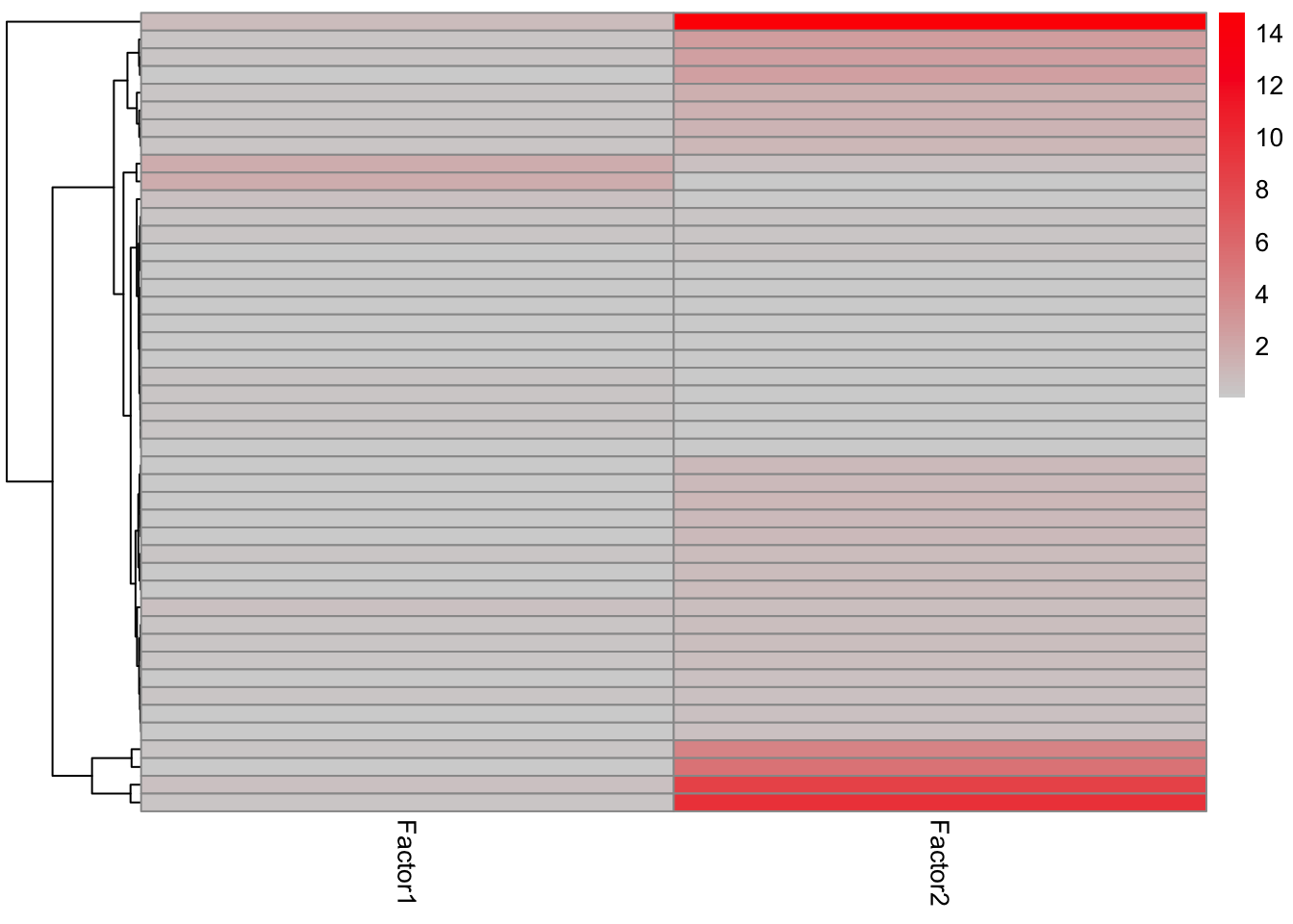
enRes.KEGG <- run_enrichment(MOFAobject, view =  "prot", factors = c(1,2), feature.sets = sigMat$KEGG, set.statistic = "mean.diff",
                          sign = "all", verbose = FALSE)
plot_enrichment_heatmap(enRes.KEGG)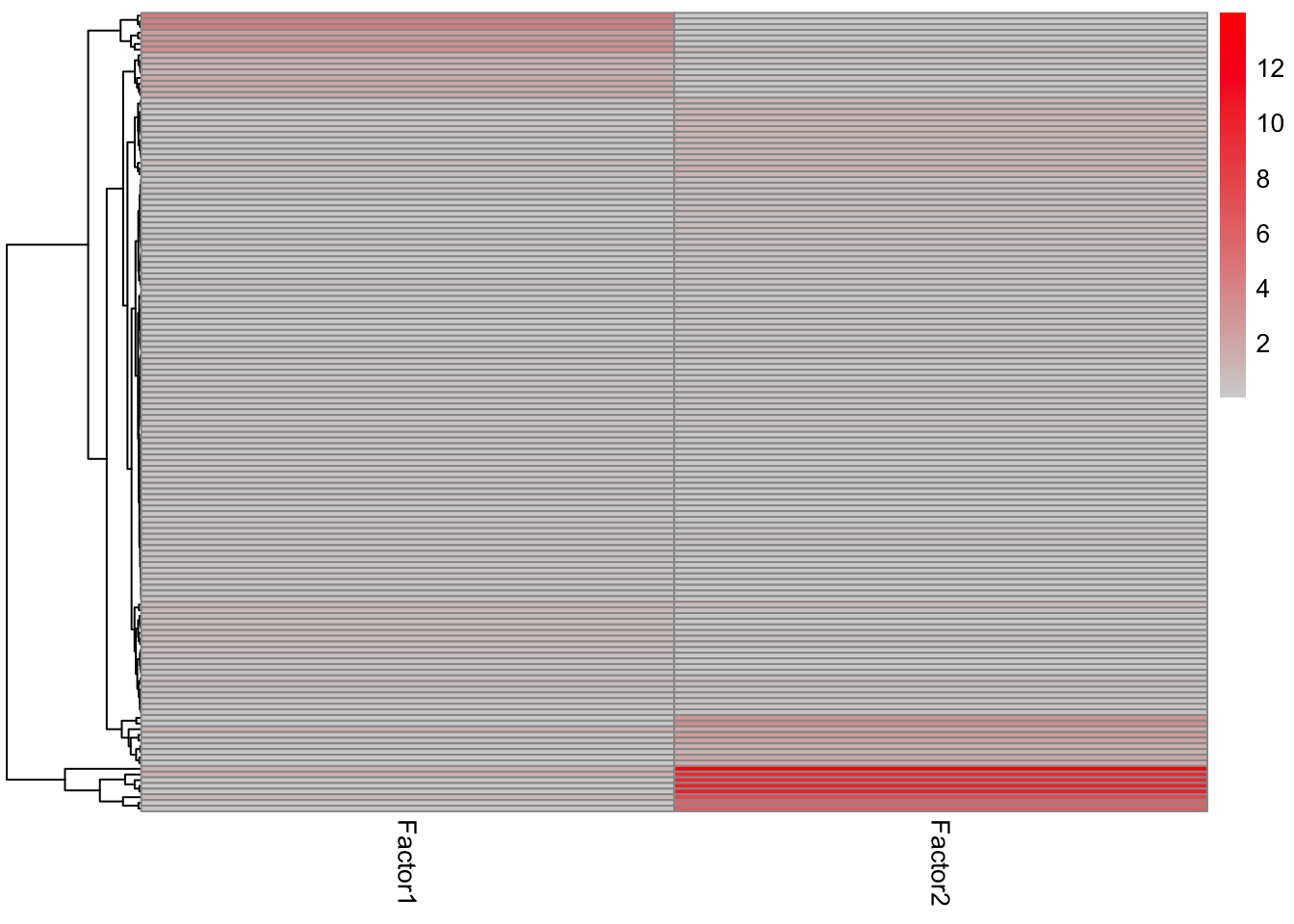
enRes.BP <- run_enrichment(MOFAobject, view =  "prot", factors = c(1,2), feature.sets = sigMat$GOBP, set.statistic = "mean.diff",
                          sign = "all", verbose = FALSE)
plot_enrichment_heatmap(enRes.BP)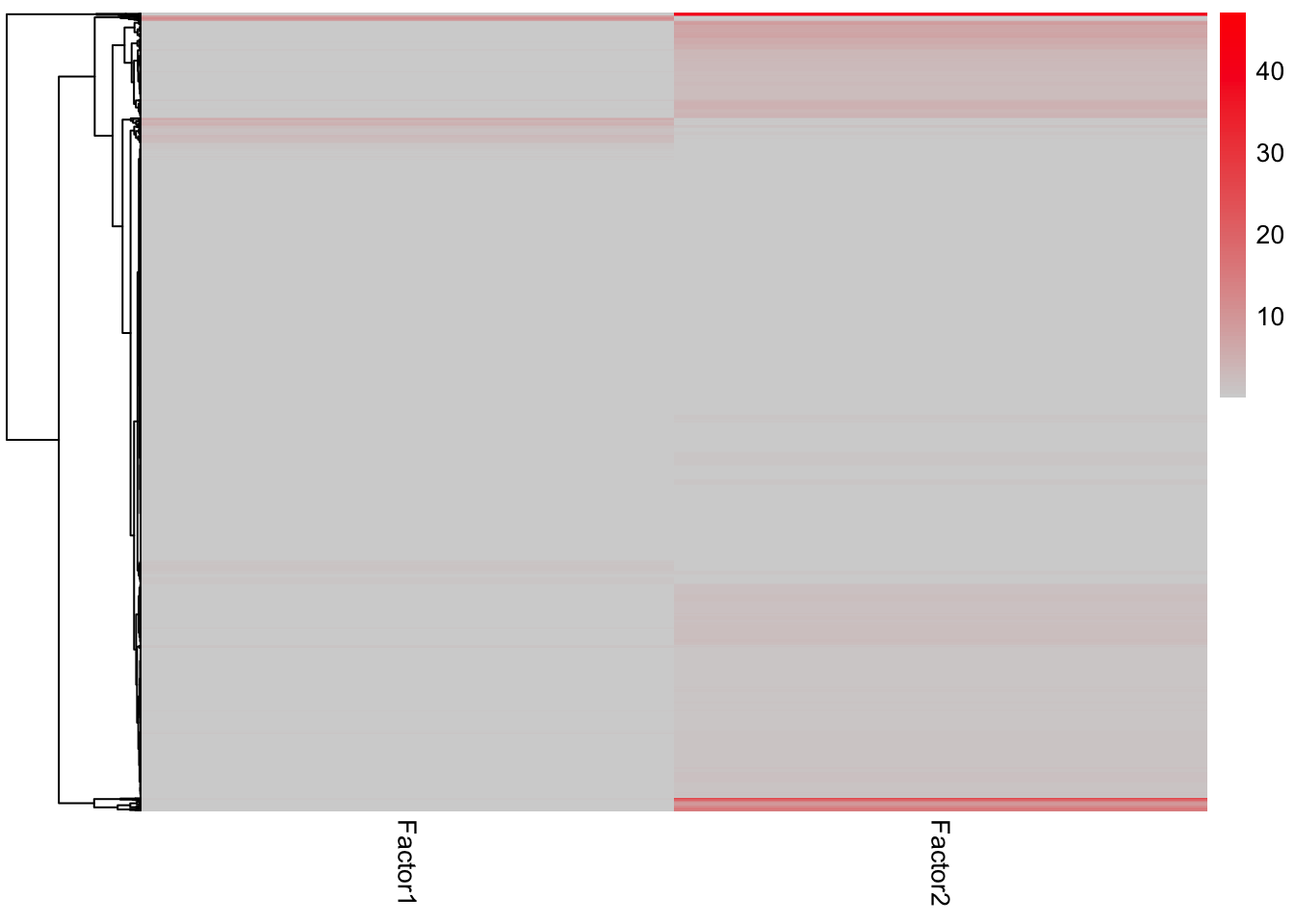
enRes.C6 <- run_enrichment(MOFAobject, view =  "prot", factors = c(1,2), feature.sets = sigMat$C6, set.statistic = "mean.diff",
                          sign = "all", verbose = FALSE)
plot_enrichment_heatmap(enRes.C6)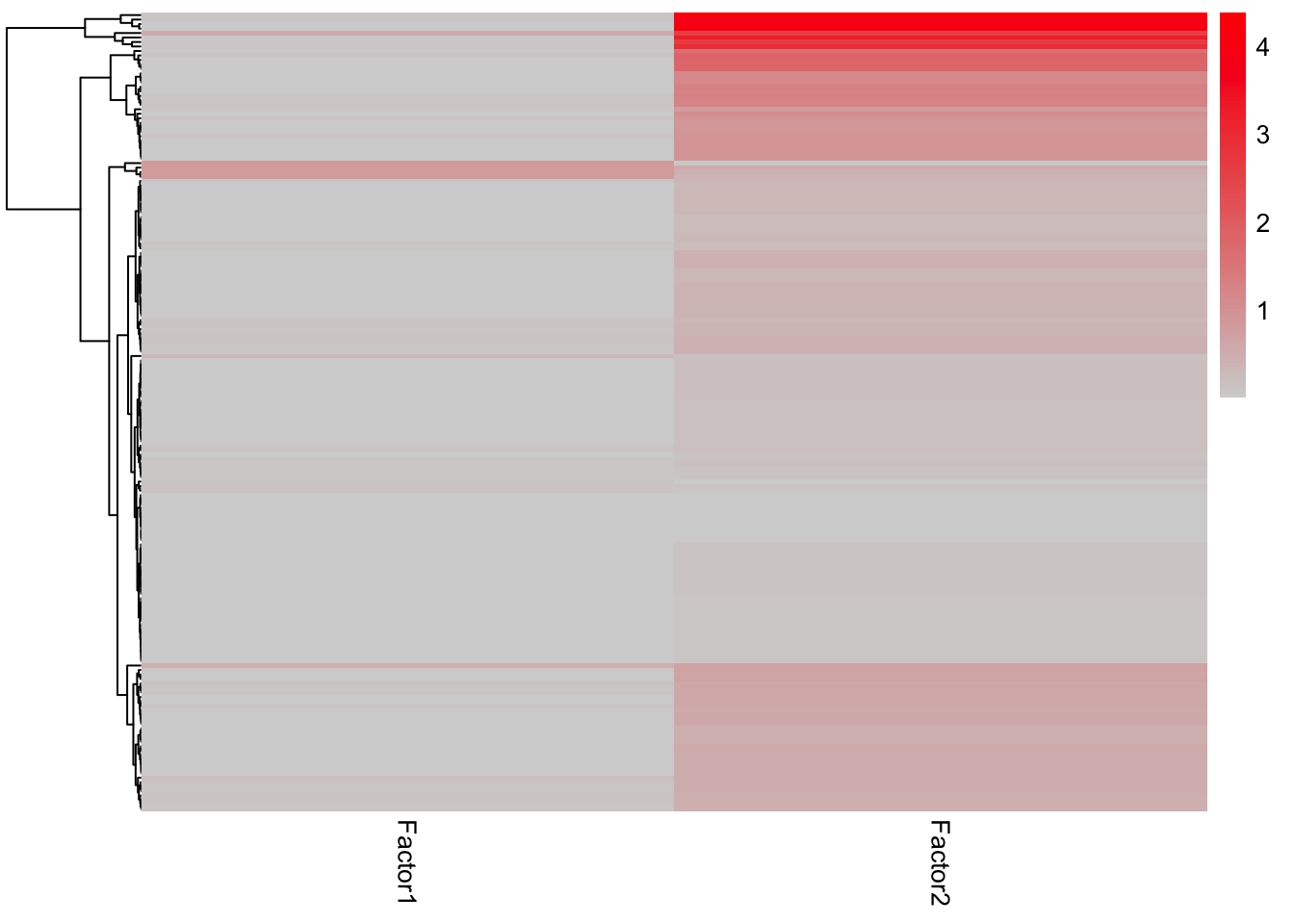
Factor 1
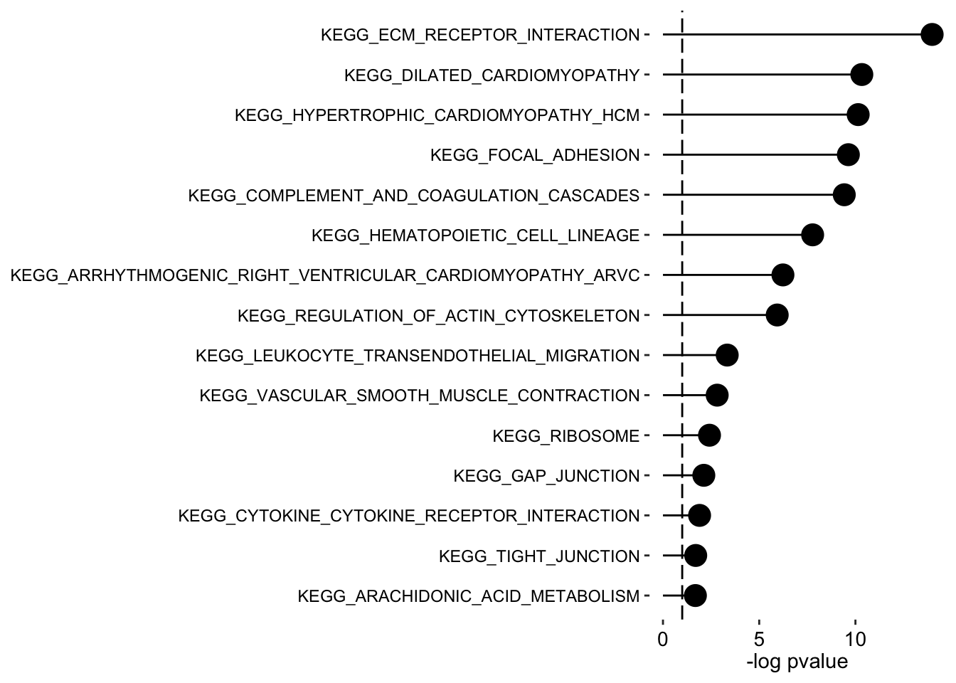
plot_enrichment(enRes.KEGG,
  max.pathways = 15,
  factor = "Factor1",
  alpha = 0.1
)
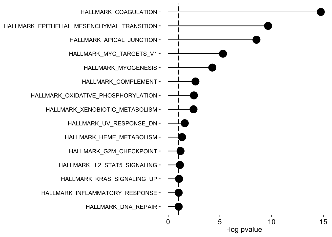
plot_enrichment(enRes.H,
  max.pathways = 15,
  factor = "Factor1",
  alpha = 0.1
)
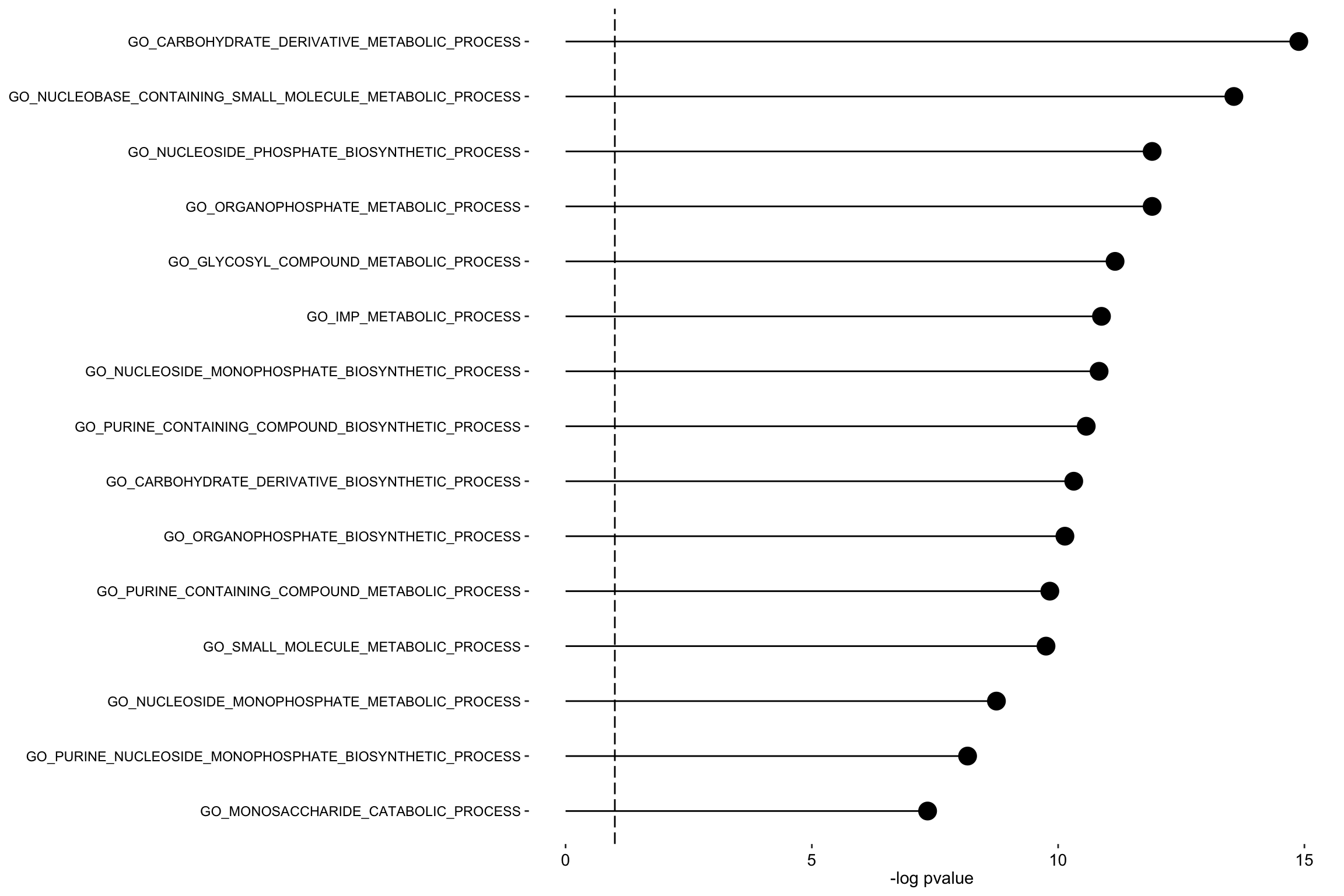
plot_enrichment(enRes.BP,
  max.pathways = 15,
  factor = "Factor1",
  alpha = 0.1
)
Factor 2
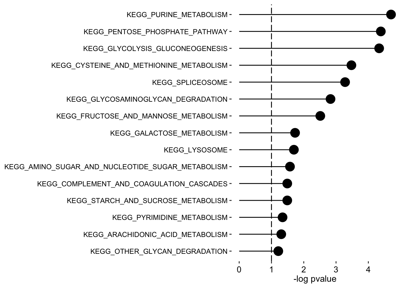
plot_enrichment(enRes.KEGG,
  max.pathways = 15,
  factor = "Factor2",
  alpha = 0.1
)
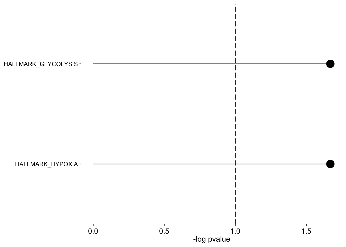
plot_enrichment(enRes.H,
  max.pathways = 15,
  factor = "Factor2",
  alpha = 0.1
)
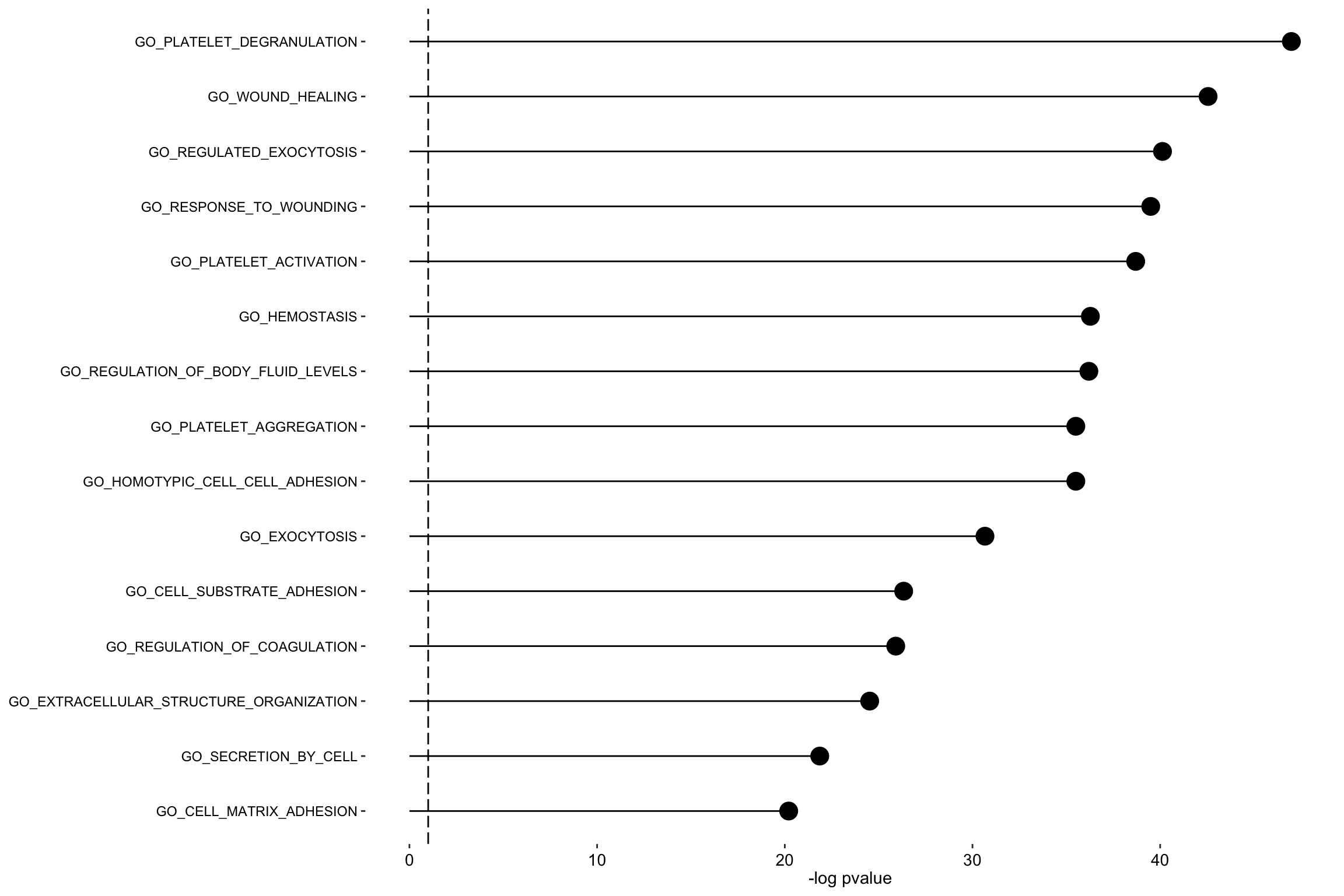
plot_enrichment(enRes.BP,
  max.pathways = 15,
  factor = "Factor2",
  alpha = 0.1
)
Only use DIA proteomic, methylation and metabolomics
Create MAE object for mofa
mofaMae <- MultiAssayExperiment(experiments = list(meta = metaMat, prot = protMat, meth = methMat),
                                colData = colData(maeObj))
Only keep samples that have at least four assays
useSamples <- MultiAssayExperiment::sampleMap(mofaMae) %>%
  as_tibble() %>% group_by(primary) %>% summarise(n= length(assay)) %>%
  filter(n >= 2) %>% pull(primary)
mofaMae <- mofaMae[,useSamples]
MOFAobject <- create_mofa_from_MultiAssayExperiment(mofaMae)Plot data overview
plot_data_overview(MOFAobject)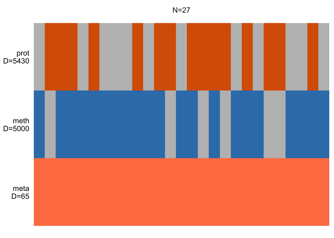
Define MOFA options
Data options
data_opts <- get_default_data_options(MOFAobject)
data_opts
$scale_views
[1] FALSE
$scale_groups
[1] FALSE
$center_groups
[1] TRUE
$use_float32
[1] FALSE
$views
[1] "meta" "prot" "meth"
$groups
[1] "group1"Model options
model_opts <- get_default_model_options(MOFAobject)
#model_opts$spikeslab_weights <- FALSE

model_opts$num_factors <- 6
model_opts
$likelihoods
meta prot meth
"gaussian" "gaussian" "gaussian"
$num_factors
[1] 6
$spikeslab_factors
[1] FALSE
$spikeslab_weights
[1] TRUE
$ard_factors
[1] FALSE
$ard_weights
[1] TRUETraining options
train_opts <- get_default_training_options(MOFAobject)
train_opts$convergence_mode <- "slow"
train_opts$seed <- 2022
train_opts$maxiter <- 10000
train_opts
$maxiter
[1] 10000
$convergence_mode
[1] "slow"
$drop_factor_threshold
[1] -1
$verbose
[1] FALSE
$startELBO
[1] 1
$freqELBO
[1] 5
$stochastic
[1] FALSE
$gpu_mode
[1] FALSE
$seed
[1] 2022
$outfile
NULL
$weight_views
[1] FALSE
$save_interrupted
[1] FALSEChange drop threshold to 0.01
train_opts$drop_factor_threshold <-0.01Train the MOFA model
Prepare MOFA object
MOFAobject <- prepare_mofa(MOFAobject,
  data_options = data_opts,
  model_options = model_opts,
  training_options = train_opts
)
Add usefull metadata
sampleTab <- colData(mofaMae) %>% data.frame() %>% rownames_to_column("sample") %>% dplyr::rename(phenotype = group)
samples_metadata(MOFAobject) <- sampleTab
Training
MOFAobject <- run_mofa(MOFAobject)
saveRDS(MOFAobject,"../output/mofaOut_small.rds")
Preliminary analysis of the results
MOFAobject <- readRDS("../output/mofaOut_small.rds")Factor correlation matrix
plot_factor_cor(MOFAobject)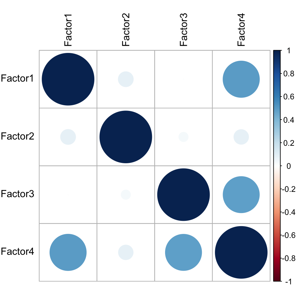
Variance explained
plot_variance_explained(MOFAobject, max_r2=15)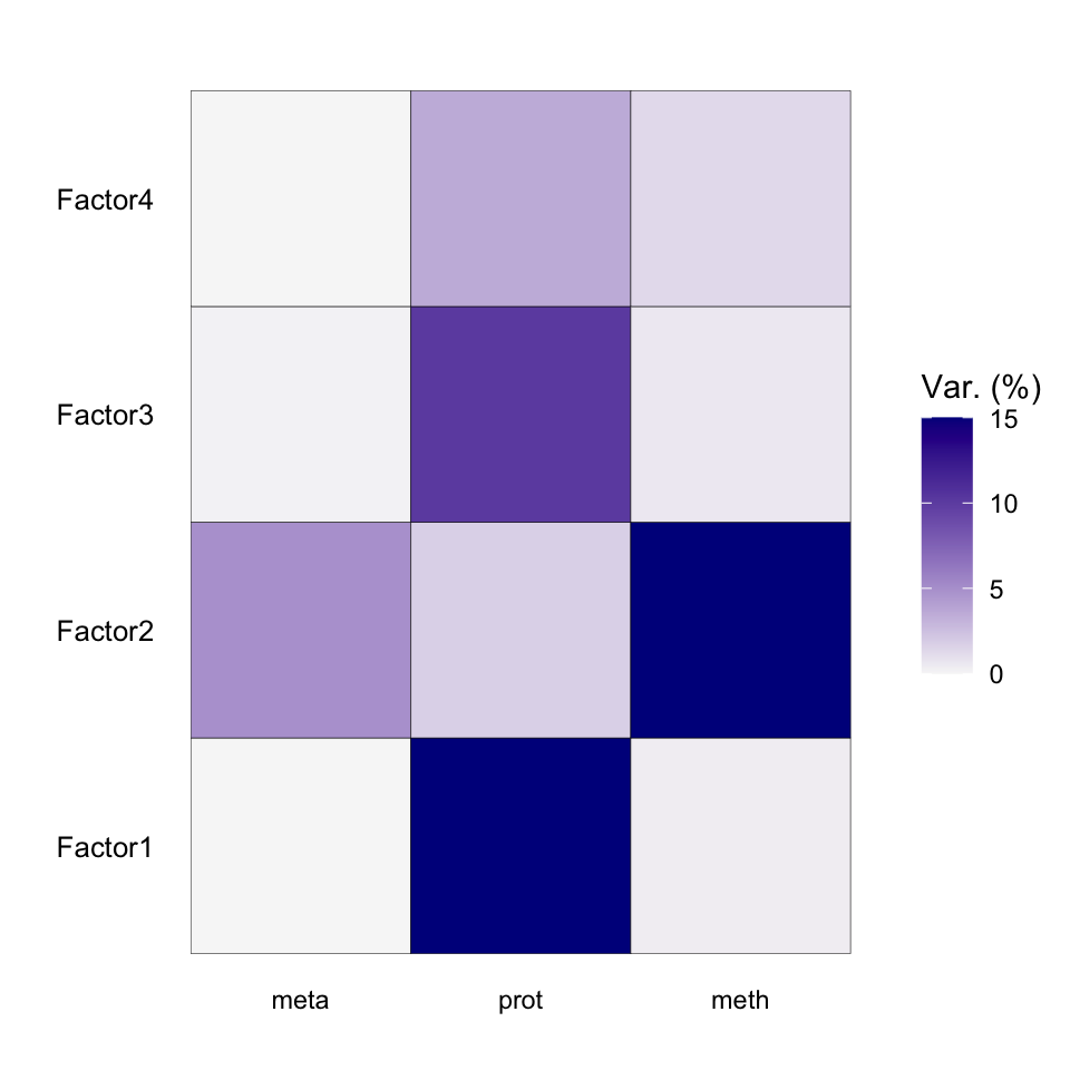
Total variance explained
plot_variance_explained(MOFAobject, plot_total = T)[[2]]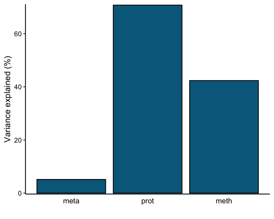
correlate_factors_with_covariates(MOFAobject,
  plot="log_pval",
  covariates = c("Gender","phenotype", "Age","CCP","GC","Leflunomid","MTX", "Quensyl","RF","Sulfasalazin","CRP","DAS28"))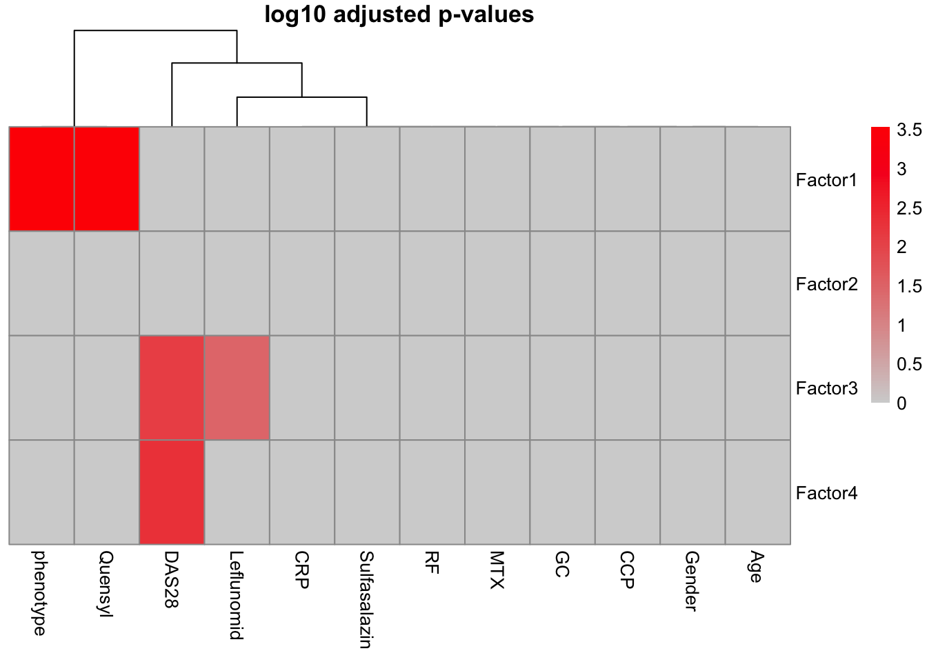
T-test
facTab <- get_factors(MOFAobject, groups = "group1", as.data.frame = TRUE) %>%
    mutate(phenotype = colData(mofaMae)[sample,]$group)

resTab <- facTab %>% group_by(factor) %>% nest() %>%
    mutate(m=map(data, ~t.test(value~phenotype, data=., var.equal=TRUE))) %>%
    mutate(res = map(m, broom::tidy)) %>%
    unnest(res) %>%
    select(factor, estimate, p.value)
resTab
# A tibble: 4 × 3
# Groups: factor [4]
factor estimate p.value
<fct> <dbl> <dbl>
1 Factor1 1.75 0.000295
2 Factor2 -0.279 0.763
3 Factor3 -0.278 0.475
4 Factor4 -0.387 0.352 plotTab <- select(facTab, factor, sample, value, phenotype) %>%
filter(factor %in% c("Factor1","Factor2")) %>%
pivot_wider(names_from = factor, values_from = value)
ggplot(plotTab, aes(x=Factor1, y=Factor2, color = phenotype)) +
geom_point() +
ggrepel::geom_text_repel(aes(label = sample)) +
theme_bw()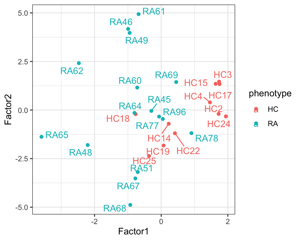
sessionInfo()R version 4.2.0 (2022-04-22)
Platform: x86_64-apple-darwin17.0 (64-bit)
Running under: macOS Big Sur/Monterey 10.16
Matrix products: default
BLAS: /Library/Frameworks/R.framework/Versions/4.2/Resources/lib/libRblas.0.dylib
LAPACK: /Library/Frameworks/R.framework/Versions/4.2/Resources/lib/libRlapack.dylib
locale:
[1] en_US.UTF-8/en_US.UTF-8/en_US.UTF-8/C/en_US.UTF-8/en_US.UTF-8
attached base packages:
[1] stats4 stats graphics grDevices utils datasets methods
[8] base
other attached packages:
[1] forcats_0.5.1 stringr_1.4.1
[3] dplyr_1.1.4.9000 purrr_0.3.4
[5] readr_2.1.2 tidyr_1.2.0
[7] tibble_3.2.1 ggplot2_3.4.1
[9] tidyverse_1.3.2 MOFA2_1.6.0
[11] MultiAssayExperiment_1.22.0 SummarizedExperiment_1.26.1
[13] Biobase_2.56.0 GenomicRanges_1.48.0
[15] GenomeInfoDb_1.32.2 IRanges_2.30.0
[17] S4Vectors_0.34.0 BiocGenerics_0.42.0
[19] MatrixGenerics_1.8.1 matrixStats_0.62.0
[21] jyluMisc_0.1.5
loaded via a namespace (and not attached):
[1] utf8_1.2.4 shinydashboard_0.7.2 reticulate_1.25
[4] tidyselect_1.2.1 RSQLite_2.2.15 AnnotationDbi_1.58.0
[7] htmlwidgets_1.5.4 grid_4.2.0 BiocParallel_1.30.3
[10] Rtsne_0.16 maxstat_0.7-25 munsell_0.5.0
[13] preprocessCore_1.58.0 codetools_0.2-18 DT_0.23
[16] withr_3.0.0 colorspace_2.0-3 filelock_1.0.2
[19] highr_0.9 knitr_1.39 rstudioapi_0.13
[22] ggsignif_0.6.3 labeling_0.4.2 git2r_0.30.1
[25] slam_0.1-50 GenomeInfoDbData_1.2.8 mnormt_2.1.0
[28] KMsurv_0.1-5 farver_2.1.1 bit64_4.0.5
[31] pheatmap_1.0.12 rhdf5_2.40.0 rprojroot_2.0.3
[34] basilisk_1.8.0 vctrs_0.6.5 generics_0.1.3
[37] TH.data_1.1-1 xfun_0.31 sets_1.0-21
[40] R6_2.5.1 bitops_1.0-7 rhdf5filters_1.8.0
[43] cachem_1.0.6 fgsea_1.22.0 DelayedArray_0.22.0
[46] assertthat_0.2.1 promises_1.2.0.1 scales_1.2.0
[49] multcomp_1.4-19 googlesheets4_1.0.0 gtable_0.3.0
[52] affy_1.74.0 sandwich_3.0-2 workflowr_1.7.0
[55] rlang_1.1.3 genefilter_1.78.0 splines_4.2.0
[58] rstatix_0.7.0 gargle_1.2.0 broom_1.0.0
[61] BiocManager_1.30.18 yaml_2.3.5 reshape2_1.4.4
[64] abind_1.4-5 modelr_0.1.8 backports_1.4.1
[67] httpuv_1.6.6 tools_4.2.0 relations_0.6-12
[70] psych_2.2.5 affyio_1.66.0 ellipsis_0.3.2
[73] gplots_3.1.3 jquerylib_0.1.4 RColorBrewer_1.1-3
[76] Rcpp_1.0.9 plyr_1.8.7 visNetwork_2.1.0
[79] zlibbioc_1.42.0 RCurl_1.98-1.7 basilisk.utils_1.8.0
[82] ggpubr_0.4.0 cowplot_1.1.1 zoo_1.8-10
[85] haven_2.5.0 ggrepel_0.9.1 cluster_2.1.3
[88] exactRankTests_0.8-35 fs_1.5.2 magrittr_2.0.3
[91] data.table_1.14.8 reprex_2.0.1 survminer_0.4.9
[94] googledrive_2.0.0 mvtnorm_1.1-3 hms_1.1.1
[97] shinyjs_2.1.0 mime_0.12 evaluate_0.15
[100] xtable_1.8-4 XML_3.99-0.10 readxl_1.4.0
[103] gridExtra_2.3 compiler_4.2.0 KernSmooth_2.23-20
[106] crayon_1.5.2 htmltools_0.5.4 later_1.3.0
[109] tzdb_0.3.0 lubridate_1.8.0 DBI_1.1.3
[112] corrplot_0.92 dbplyr_2.2.1 MASS_7.3-58
[115] Matrix_1.5-4 car_3.1-0 cli_3.6.2
[118] vsn_3.64.0 marray_1.74.0 parallel_4.2.0
[121] igraph_1.3.4 pkgconfig_2.0.3 km.ci_0.5-6
[124] dir.expiry_1.4.0 piano_2.12.0 xml2_1.3.3
[127] annotate_1.74.0 bslib_0.4.1 XVector_0.36.0
[130] drc_3.0-1 rvest_1.0.2 digest_0.6.30
[133] Biostrings_2.64.0 rmarkdown_2.14 cellranger_1.1.0
[136] fastmatch_1.1-3 survMisc_0.5.6 uwot_0.1.11
[139] shiny_1.7.4 gtools_3.9.3 nlme_3.1-158
[142] lifecycle_1.0.4 jsonlite_1.8.3 Rhdf5lib_1.18.2
[145] carData_3.0-5 limma_3.52.2 fansi_1.0.6
[148] pillar_1.9.0 lattice_0.20-45 KEGGREST_1.36.3
[151] fastmap_1.1.0 httr_1.4.3 plotrix_3.8-2
[154] survival_3.4-0 glue_1.7.0 png_0.1-7
[157] bit_4.0.4 stringi_1.7.8 sass_0.4.2
[160] HDF5Array_1.24.1 blob_1.2.3 memoise_2.0.1
[163] caTools_1.18.2