Analysis of the cytokine data of the keto diet cohort and aKG treated samples
Junyan Lu
Last updated: 2024-05-24
Checks: 5 1
Knit directory: RA_Tcell_omics/analysis/
This reproducible R Markdown analysis was created with workflowr (version 1.7.0). The Checks tab describes the reproducibility checks that were applied when the results were created. The Past versions tab lists the development history.
Great job! The global environment was empty. Objects defined in the global environment can affect the analysis in your R Markdown file in unknown ways. For reproduciblity it’s best to always run the code in an empty environment.
The command set.seed(20221110) was run prior to running
the code in the R Markdown file. Setting a seed ensures that any results
that rely on randomness, e.g. subsampling or permutations, are
reproducible.
Great job! Recording the operating system, R version, and package versions is critical for reproducibility.
Nice! There were no cached chunks for this analysis, so you can be confident that you successfully produced the results during this run.
Great job! Using relative paths to the files within your workflowr project makes it easier to run your code on other machines.
Tracking code development and connecting the code version to the
results is critical for reproducibility. To start using Git, open the
Terminal and type git init in your project directory.
This project is not being versioned with Git. To obtain the full
reproducibility benefits of using workflowr, please see
?wflow_start.
Load libraries
Process cytokine data
cytoTab <- read_delim("../data/Cytokines_Keto_and_invitro_normalized_to_cellcount.csv", col_types = "cccccccccccccc") %>%
  mutate(across(-well, as.numeric)) %>%
  pivot_longer(-well, names_to = "cytokine", values_to = "value") %>%
  mutate(patID = str_extract(well, "(K|RA)[0-9]*"),
         time = str_extract(well, "d[0-9]*"),
         group = str_extract(well, "st|ns|aKG")) %>%
  mutate(diseaseGroup = ifelse(patID %in% c("K11","K13","K16"),"dCNT","RA")) %>% #11,13,16 are disease controls
  mutate(log2Val = glog2(value))
QA
Boxplot showing the value distribution
Original scale
ggplot(cytoTab, aes(x=cytokine, y = value)) +
  geom_boxplot() +
  geom_point() +
  theme(axis.text.x = element_text(angle = 90, hjust = 1, vjust = 0.5))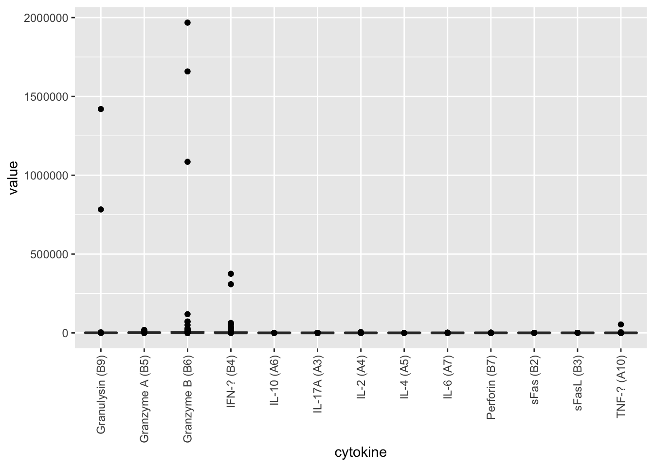
log2 scale
ggplot(cytoTab, aes(x=cytokine, y = log2Val)) +
geom_boxplot() +
geom_point() +
theme(axis.text.x = element_text(angle = 90, hjust = 1, vjust = 0.5))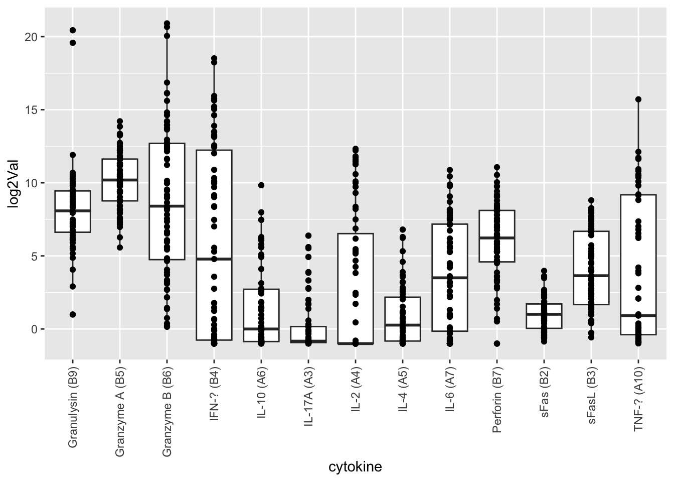 Tests need to be performed on log2 scale, which is more normally
distributed
Tests need to be performed on log2 scale, which is more normally
distributed
Identify cytokines associated with keto diet
ketoTab <- filter(cytoTab, !is.na(time))In RA patient samples
Unstimutated samples
testTab <- filter(ketoTab, group == "ns", diseaseGroup == "RA")
resTab <- group_by(testTab, cytokine) %>% nest() %>%
  mutate(m = map(data, ~summary(lm(log2Val ~ patID + time,.)))) %>%
  mutate(res = map(m, broom::tidy)) %>%
  unnest(res) %>%
  filter(term == "timed12") %>%
  select(cytokine, p.value, statistic, estimate) %>%
  arrange(p.value)

head(resTab)
# A tibble: 6 × 4
# Groups: cytokine [6]
cytokine p.value statistic estimate
<chr> <dbl> <dbl> <dbl>
1 Granzyme A (B5) 0.430 -0.846 -0.580
2 Granzyme B (B6) 0.430 -0.846 -0.852
3 Granulysin (B9) 0.466 -0.778 -0.680
4 IL-10 (A6) 0.645 -0.485 -0.331
5 IL-6 (A7) 0.647 -0.482 -0.523
6 IFN-? (B4) 0.659 0.464 0.229No associations passed p<0.05
Stimulated samples
testTab <- filter(ketoTab, group == "st", diseaseGroup == "RA")
resTab <- group_by(testTab, cytokine) %>% nest() %>%
  mutate(m = map(data, ~summary(lm(log2Val ~ patID + time,.)))) %>%
  mutate(res = map(m, broom::tidy)) %>%
  unnest(res) %>%
  filter(term == "timed12") %>%
  select(cytokine, p.value, statistic, estimate) %>%
  arrange(p.value)

head(resTab)
# A tibble: 6 × 4
# Groups: cytokine [6]
cytokine p.value statistic estimate
<chr> <dbl> <dbl> <dbl>
1 Granzyme B (B6) 0.140 1.70 0.803
2 Granulysin (B9) 0.171 -1.55 -0.961
3 Granzyme A (B5) 0.217 -1.38 -0.676
4 IL-2 (A4) 0.292 1.16 0.955
5 IL-6 (A7) 0.319 -1.09 -1.08
6 sFas (B2) 0.331 -1.06 -0.578In disease control samples
Unstimutated samples
testTab <- filter(ketoTab, group == "ns", diseaseGroup == "dCNT")
resTab <- group_by(testTab, cytokine) %>% nest() %>%
  mutate(m = map(data, ~summary(lm(log2Val ~ patID + time,.)))) %>%
  mutate(res = map(m, broom::tidy)) %>%
  unnest(res) %>%
  filter(term == "timed12") %>%
  select(cytokine, p.value, statistic, estimate) %>%
  arrange(p.value)

head(resTab)
# A tibble: 6 × 4
# Groups: cytokine [6]
cytokine p.value statistic estimate
<chr> <dbl> <dbl> <dbl>
1 sFasL (B3) 0.152 -2.26 -2.23e- 1
2 IL-6 (A7) 0.266 -1.53 -1.07e+ 0
3 Granulysin (B9) 0.310 -1.35 -5.59e- 1
4 TNF-? (A10) 0.399 1.06 3.29e- 1
5 IL-2 (A4) 0.423 1 1.81e-16
6 IL-10 (A6) 0.423 -0.998 -4.38e- 1No associations passed p<0.05
Stimulated samples
testTab <- filter(ketoTab, group == "st", diseaseGroup == "dCNT")
resTab <- group_by(testTab, cytokine) %>% nest() %>%
  mutate(m = map(data, ~summary(lm(log2Val ~ patID + time,.)))) %>%
  mutate(res = map(m, broom::tidy)) %>%
  unnest(res) %>%
  filter(term == "timed12") %>%
  select(cytokine, p.value, statistic, estimate) %>%
  arrange(p.value)

head(resTab)
# A tibble: 6 × 4
# Groups: cytokine [6]
cytokine p.value statistic estimate
<chr> <dbl> <dbl> <dbl>
1 IL-4 (A5) 0.0202 -6.93 -1.44
2 IL-6 (A7) 0.0484 -4.38 -4.60
3 Granzyme A (B5) 0.0759 -3.42 -1.49
4 IL-10 (A6) 0.0779 -3.37 -1.61
5 IL-17A (A3) 0.0867 -3.17 -2.06
6 TNF-? (A10) 0.141 -2.38 -1.01Two passed P < 0.05
resTab.sig <- filter(resTab, p.value < 0.05)
pList <- lapply(seq(nrow(resTab.sig)), function(i) {
  rec <- resTab.sig[i,]
  plotTab <- filter(testTab, cytokine == rec$cytokine)
  ggplot(plotTab, aes(x=time, y=log2Val)) +
    geom_line(aes(group = patID)) +
    geom_point() +
    ggtitle(sprintf("%s (P=%s)",rec$cytokine, formatC(rec$p.value, digits = 2))) +
    ylab("Log2 expression") + xlab("")
})

cowplot::plot_grid(plotlist = pList, ncol=2)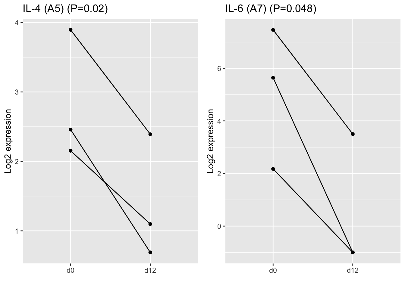
Identify cytokines associated aKG supplement in RA samples
aKG group versus st group
testTab <- filter(cytoTab, is.na(time), group %in% c("st","aKG")) %>%
  mutate(group = factor(group, levels = c("st","aKG")))
resTab <- group_by(testTab, cytokine) %>% nest() %>%
mutate(m = map(data, ~summary(lm(log2Val ~ patID + group,.)))) %>%
mutate(res = map(m, broom::tidy)) %>%
unnest(res) %>%
filter(term == "groupaKG") %>%
select(cytokine, p.value, statistic, estimate) %>%
arrange(p.value)Associations passed P< 0.05
resTab.sig <- filter(resTab, p.value < 0.05)
resTab.sig %>% mutate_if(is.numeric, formatC, digits=2) %>% DT::datatable()
Plot changes
pList <- lapply(seq(nrow(resTab.sig)), function(i) {
  rec <- resTab.sig[i,]
  plotTab <- filter(testTab, cytokine == rec$cytokine)
  ggplot(plotTab, aes(x=group, y=log2Val)) +
    geom_line(aes(group = patID)) +
    geom_point() +
    ggtitle(sprintf("%s (P=%s)",rec$cytokine, formatC(rec$p.value, digits = 2))) +
    ylab("Log2 expression") + xlab("")
})

cowplot::plot_grid(plotlist = pList, ncol=3)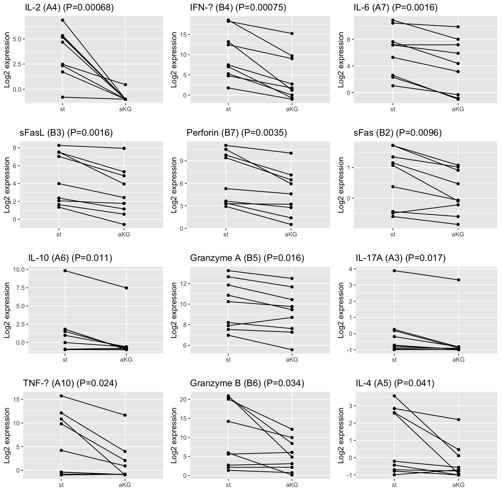
Also add ns group to the visualization
visTab <- filter(cytoTab, is.na(time), group %in% c("ns","st","aKG")) %>%
mutate(group = factor(group, levels = c("ns","st","aKG")))
pList <- lapply(seq(nrow(resTab.sig)), function(i) {
rec <- resTab.sig[i,]
plotTab <- filter(visTab, cytokine == rec$cytokine)
ggplot(plotTab, aes(x=group, y=log2Val)) +
geom_line(aes(group = patID)) +
geom_point() +
ggtitle(sprintf("%s (P=%s)",rec$cytokine, formatC(rec$p.value, digits = 2))) +
ylab("Log2 expression") + xlab("")
})
cowplot::plot_grid(plotlist = pList, ncol=3)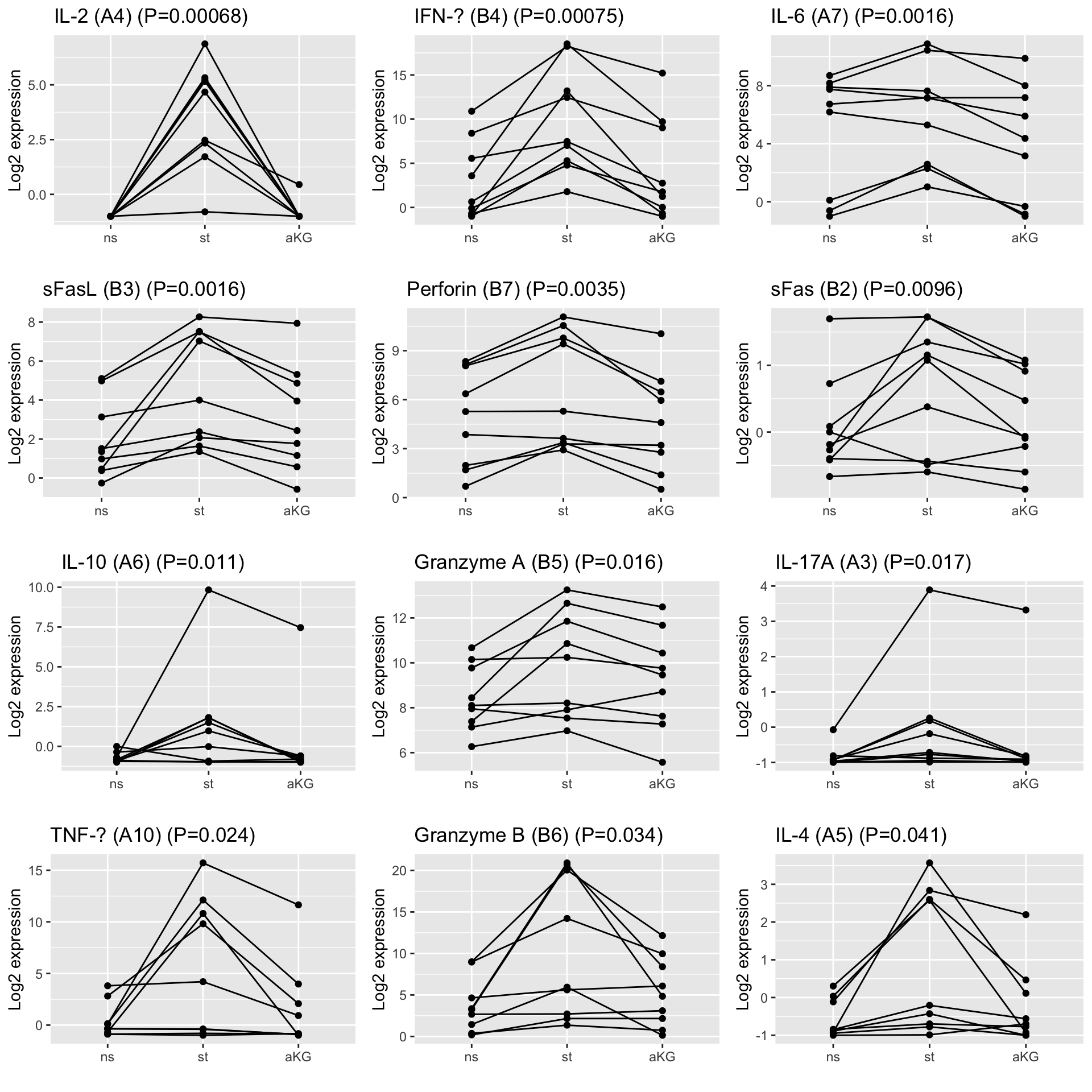 It seems aKG can reverse many of the stimulation
effect.
It seems aKG can reverse many of the stimulation
effect.
st group versus ns group
testTab <- filter(cytoTab, is.na(time), group %in% c("st","ns")) %>%
  mutate(group = factor(group, levels = c("ns","st")))
resTab <- group_by(testTab, cytokine) %>% nest() %>%
mutate(m = map(data, ~summary(lm(log2Val ~ patID + group,.)))) %>%
mutate(res = map(m, broom::tidy)) %>%
unnest(res) %>%
filter(term == "groupst") %>%
select(cytokine, p.value, statistic, estimate) %>%
arrange(p.value)Associations passed P<0.05
resTab.sig <- filter(resTab, p.value < 0.05)
resTab.sig %>% mutate_if(is.numeric, formatC, digits=2) %>% DT::datatable()
Plot changes
pList <- lapply(seq(nrow(resTab.sig)), function(i) {
  rec <- resTab.sig[i,]
  plotTab <- filter(testTab, cytokine == rec$cytokine)
  ggplot(plotTab, aes(x=group, y=log2Val)) +
    geom_line(aes(group = patID)) +
    geom_point() +
    ggtitle(sprintf("%s (P=%s)",rec$cytokine, formatC(rec$p.value, digits = 2))) +
    ylab("Log2 expression") + xlab("")
})

cowplot::plot_grid(plotlist = pList, ncol=3)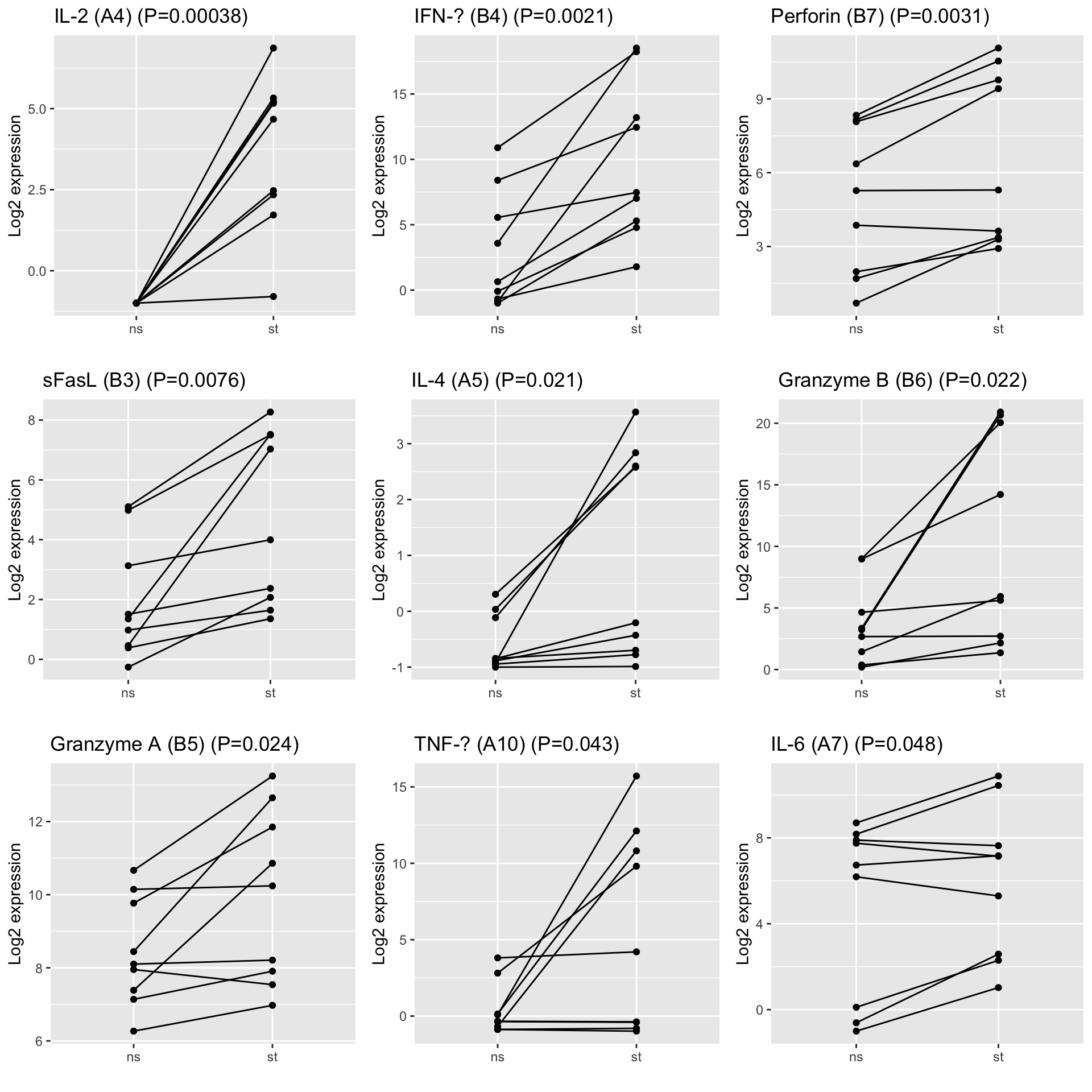
sessionInfo()R version 4.2.0 (2022-04-22)
Platform: x86_64-apple-darwin17.0 (64-bit)
Running under: macOS Big Sur/Monterey 10.16
Matrix products: default
BLAS: /Library/Frameworks/R.framework/Versions/4.2/Resources/lib/libRblas.0.dylib
LAPACK: /Library/Frameworks/R.framework/Versions/4.2/Resources/lib/libRlapack.dylib
locale:
[1] en_US.UTF-8/en_US.UTF-8/en_US.UTF-8/C/en_US.UTF-8/en_US.UTF-8
attached base packages:
[1] stats4 stats graphics grDevices utils datasets methods
[8] base
other attached packages:
[1] forcats_0.5.1 stringr_1.4.1
[3] dplyr_1.1.4.9000 purrr_0.3.4
[5] readr_2.1.2 tidyr_1.2.0
[7] tibble_3.2.1 ggplot2_3.4.1
[9] tidyverse_1.3.2 MultiAssayExperiment_1.22.0
[11] SummarizedExperiment_1.26.1 Biobase_2.56.0
[13] GenomicRanges_1.48.0 GenomeInfoDb_1.32.2
[15] IRanges_2.30.0 S4Vectors_0.34.0
[17] BiocGenerics_0.42.0 MatrixGenerics_1.8.1
[19] matrixStats_0.62.0 jyluMisc_0.1.5
loaded via a namespace (and not attached):
[1] readxl_1.4.0 backports_1.4.1 fastmatch_1.1-3
[4] drc_3.0-1 workflowr_1.7.0 igraph_1.3.4
[7] shinydashboard_0.7.2 splines_4.2.0 crosstalk_1.2.0
[10] BiocParallel_1.30.3 TH.data_1.1-1 digest_0.6.30
[13] htmltools_0.5.4 fansi_1.0.6 magrittr_2.0.3
[16] googlesheets4_1.0.0 cluster_2.1.3 tzdb_0.3.0
[19] limma_3.52.2 modelr_0.1.8 vroom_1.5.7
[22] sandwich_3.0-2 piano_2.12.0 colorspace_2.0-3
[25] rvest_1.0.2 haven_2.5.0 xfun_0.31
[28] crayon_1.5.2 RCurl_1.98-1.7 jsonlite_1.8.3
[31] survival_3.4-0 zoo_1.8-10 glue_1.7.0
[34] survminer_0.4.9 gtable_0.3.0 gargle_1.2.0
[37] zlibbioc_1.42.0 XVector_0.36.0 DelayedArray_0.22.0
[40] car_3.1-0 abind_1.4-5 scales_1.2.0
[43] mvtnorm_1.1-3 DBI_1.1.3 relations_0.6-12
[46] rstatix_0.7.0 Rcpp_1.0.9 plotrix_3.8-2
[49] xtable_1.8-4 bit_4.0.4 km.ci_0.5-6
[52] DT_0.23 htmlwidgets_1.5.4 httr_1.4.3
[55] fgsea_1.22.0 gplots_3.1.3 ellipsis_0.3.2
[58] farver_2.1.1 pkgconfig_2.0.3 sass_0.4.2
[61] dbplyr_2.2.1 utf8_1.2.4 labeling_0.4.2
[64] tidyselect_1.2.1 rlang_1.1.3 later_1.3.0
[67] munsell_0.5.0 cellranger_1.1.0 tools_4.2.0
[70] visNetwork_2.1.0 cachem_1.0.6 cli_3.6.2
[73] generics_0.1.3 broom_1.0.0 evaluate_0.15
[76] fastmap_1.1.0 yaml_2.3.5 bit64_4.0.5
[79] knitr_1.39 fs_1.5.2 survMisc_0.5.6
[82] caTools_1.18.2 mime_0.12 slam_0.1-50
[85] xml2_1.3.3 compiler_4.2.0 rstudioapi_0.13
[88] ggsignif_0.6.3 marray_1.74.0 reprex_2.0.1
[91] bslib_0.4.1 stringi_1.7.8 highr_0.9
[94] lattice_0.20-45 Matrix_1.5-4 shinyjs_2.1.0
[97] KMsurv_0.1-5 vctrs_0.6.5 pillar_1.9.0
[100] lifecycle_1.0.4 jquerylib_0.1.4 data.table_1.14.8
[103] cowplot_1.1.1 bitops_1.0-7 httpuv_1.6.6
[106] R6_2.5.1 promises_1.2.0.1 KernSmooth_2.23-20
[109] gridExtra_2.3 codetools_0.2-18 MASS_7.3-58
[112] gtools_3.9.3 exactRankTests_0.8-35 assertthat_0.2.1
[115] rprojroot_2.0.3 withr_3.0.0 multcomp_1.4-19
[118] GenomeInfoDbData_1.2.8 parallel_4.2.0 hms_1.1.1
[121] grid_4.2.0 rmarkdown_2.14 carData_3.0-5
[124] googledrive_2.0.0 git2r_0.30.1 maxstat_0.7-25
[127] ggpubr_0.4.0 sets_1.0-21 shiny_1.7.4
[130] lubridate_1.8.0