Process metabolimic data
Junyan Lu
Last updated: 2024-05-21
Checks: 5 1
Knit directory: RA_Tcell_omics/analysis/
This reproducible R Markdown analysis was created with workflowr (version 1.7.0). The Checks tab describes the reproducibility checks that were applied when the results were created. The Past versions tab lists the development history.
Great job! The global environment was empty. Objects defined in the global environment can affect the analysis in your R Markdown file in unknown ways. For reproduciblity it’s best to always run the code in an empty environment.
The command set.seed(20221110) was run prior to running
the code in the R Markdown file. Setting a seed ensures that any results
that rely on randomness, e.g. subsampling or permutations, are
reproducible.
Great job! Recording the operating system, R version, and package versions is critical for reproducibility.
Nice! There were no cached chunks for this analysis, so you can be confident that you successfully produced the results during this run.
Great job! Using relative paths to the files within your workflowr project makes it easier to run your code on other machines.
Tracking code development and connecting the code version to the
results is critical for reproducibility. To start using Git, open the
Terminal and type git init in your project directory.
This project is not being versioned with Git. To obtain the full
reproducibility benefits of using workflowr, please see
?wflow_start.
Load libraries
library(vsn)
library(jyluMisc)
library(SummarizedExperiment)
library(tidyverse)
knitr::opts_chunk$set(warning = FALSE, message = FALSE)
source("../code/helper.R")
Read in metabolomic data
sampleTab <- readxl::read_xlsx("../data/240315_54xMS_#24-17_results.xlsx", sheet = "sampleAnno") %>%
  mutate(sampleID = sprintf("MS%02s",Label)) %>%
  dplyr::rename(patID = Name) %>%
  mutate(Time = ifelse(is.na(Time),"d0",Time),
         group = str_extract(patID,"HC|CNT|Keto")) %>%
  select(-Label)

metaTab <- readxl::read_xlsx("../data/240315_54xMS_#24-17_results.xlsx", sheet="Normalized") %>%
  pivot_longer(-Name, names_to = "sampleID", values_to = "count") %>%
  filter(Name != "Ribitol-5TMS  (internal standard, ISTD)")

#all(unique(metaTab$sampleID) %in% sampleTab$sampleID)

metaTab <- left_join(metaTab, sampleTab, by = "sampleID")
metaID <- distinct(metaTab, Name) %>% mutate(id = seq(nrow(.))) %>%
  mutate(id = paste0("meta",id))

metaTab <- left_join(metaTab, metaID, by = "Name") %>%
  mutate(count = ifelse(count <=0, NA, count),
         sampleID = paste0(patID,"_",Time)) %>%
  dplyr::rename(ID = id, time = Time, name = Name)

seMeta <- jyluMisc::tidyToSum(metaTab, rowID = "ID", colID = "sampleID",
                              values = "count",
                              annoRow = c("ID","name"),
                              annoCol = c("sampleID","patID","time","group"))
Exploratory analysis and QA
Visualize overall data distribution
Per sample
Before transformation
ggplot(metaTab, aes(x=sampleID, y=count)) +
    geom_boxplot() + geom_point(aes(col = time)) +
    theme(axis.text = element_text(angle = 90, hjust = 1, vjust = 0.5))
After simple log transformation
ggplot(metaTab, aes(x=sampleID, y=log2(count))) +
    geom_boxplot() + geom_point(aes(col = time)) +
    theme(axis.text = element_text(angle = 90, hjust = 1, vjust = 0.5))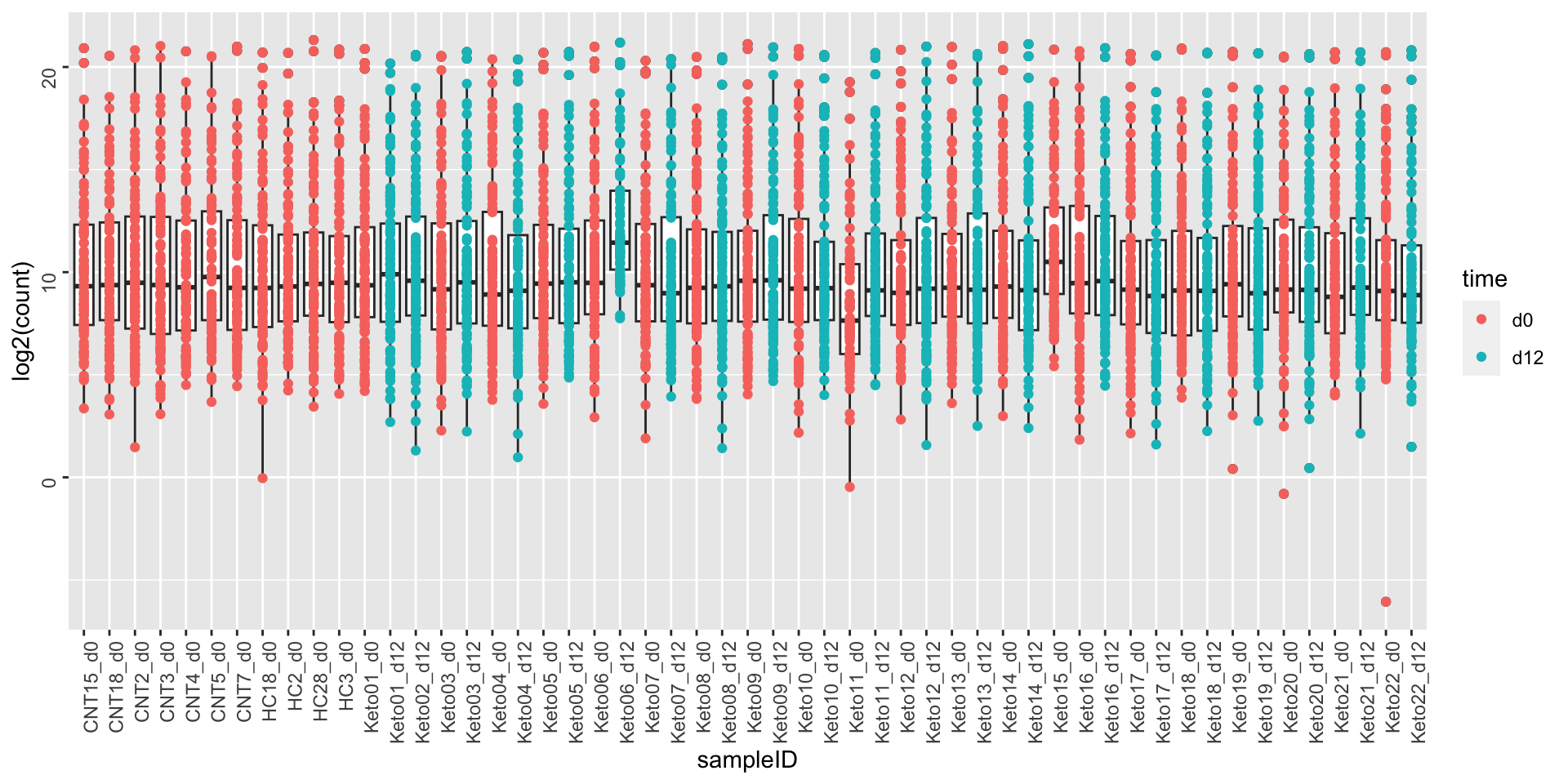
After glog2 transformation
ggplot(metaTab, aes(x=sampleID, y=glog2(count))) +
    geom_boxplot() + geom_point(aes(col = time)) +
    theme(axis.text = element_text(angle = 90, hjust = 1, vjust = 0.5))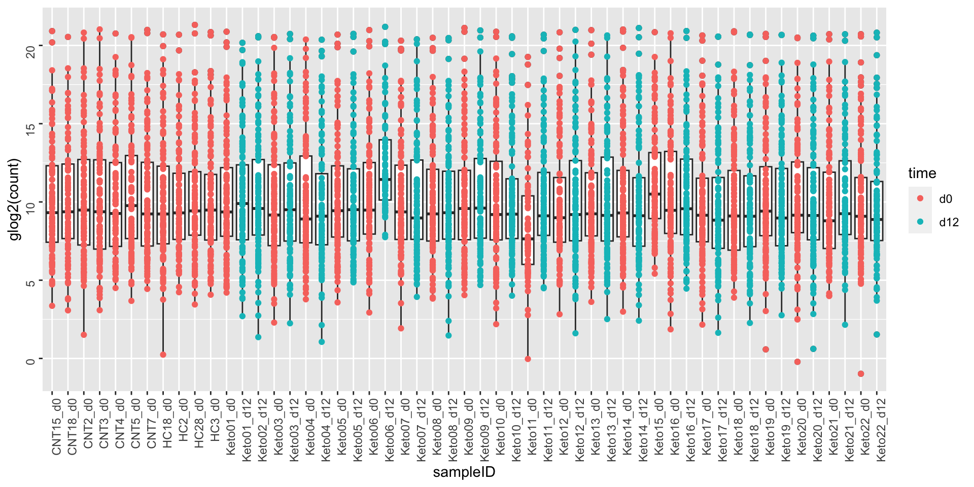
After VSN
metaMat <- assay(seMeta)
metaMat.vsn <- vsn::justvsn(metaMat)
metaTab.vsn <- as_tibble(metaMat.vsn, rownames = "ID") %>%
  pivot_longer(-ID, names_to = "sampleID", values_to = "normVsn")
metaTab <- left_join(metaTab, metaTab.vsn, by = c("ID","sampleID"))

ggplot(metaTab, aes(x=sampleID, y=normVsn)) +
    geom_boxplot() + geom_point(aes(col = time)) +
    theme(axis.text = element_text(angle = 90, hjust = 1, vjust = 0.5))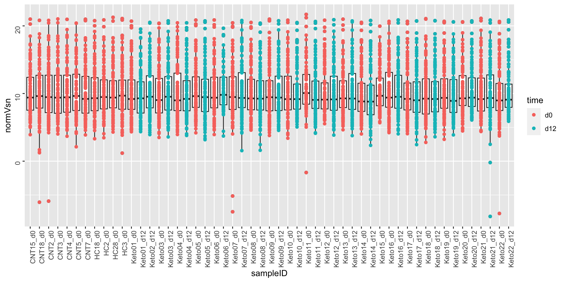
Data completeness per sample
countMat <- assay(seMeta)
plotTab <- tibble(sample = colnames(seMeta),
                  perNA = colSums(is.na(countMat))/nrow(countMat),
                  time = seMeta$time)
ggplot(plotTab, aes(x=sample, y=1-perNA)) +
    geom_bar(stat = "identity", aes(fill = time)) +
    ylab("completeness") +
    theme(axis.text.x = element_text(angle = 90, hjust = 1, vjust=0))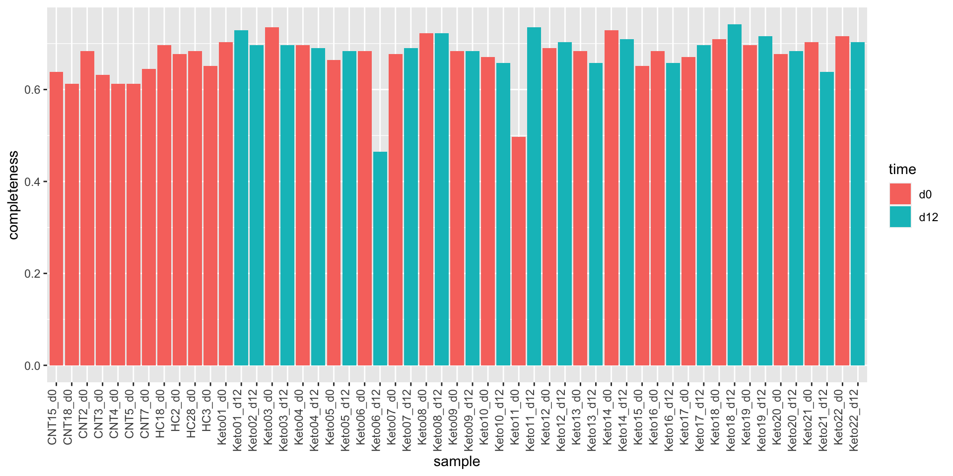
Plot a cumulative curve of missing value cut-off and remaining number of features
missRate <- tibble(id = rownames(countMat),
rate = rowSums(is.na(countMat))/ncol(countMat))
cumTab <- lapply(seq(0,1,0.05), function(cutRate) {
tibble(cut= cutRate,
per = sum(missRate$rate <= cutRate)/nrow(missRate))
} ) %>%
bind_rows()
ggplot(cumTab, aes(x=cut,y=per)) +
geom_line() +
xlab("Allowed missing value rate") +
ylab("Percentage of remaining features")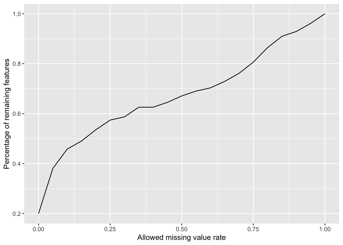 Missing value heatmap to check missing value structure
Visualize the missing value pattern
DEP::plot_missval(seMeta)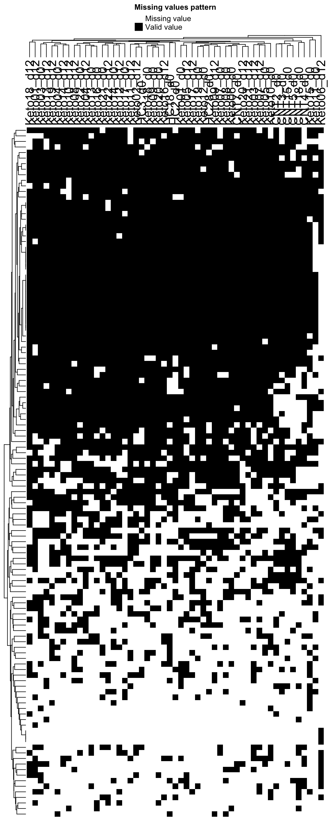
Missing value rate versus mean values
metaMat <- assay(seMeta)
plotTab <- tibble(meanVal = rowMeans(log2(metaMat), na.rm = TRUE),
                  dropRate = rowMeans(is.na(metaMat)))
ggplot(plotTab, aes(x=meanVal, y=dropRate)) +
  geom_point()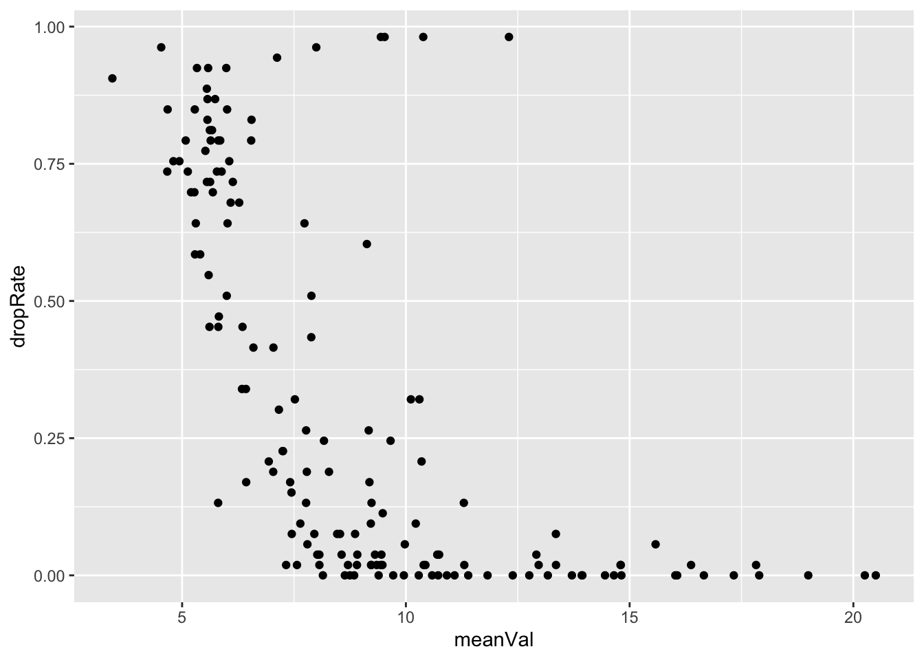
Keep metabolites detected in at least 20 percent of the samples
metaFilt <- seMeta[rowMeans(is.na(assay(seMeta))) < 0.8,]

dim(metaFilt)
[1] 134 53Imputation and normalization
transformation
metaMat <- assay(metaFilt)
#normMat <- vsn::justvsn(metaMat)
normMat <- glog2(metaMat)
metaNorm <- metaFilt
assay(metaNorm) <- normMat

vsn::meanSdPlot(normMat)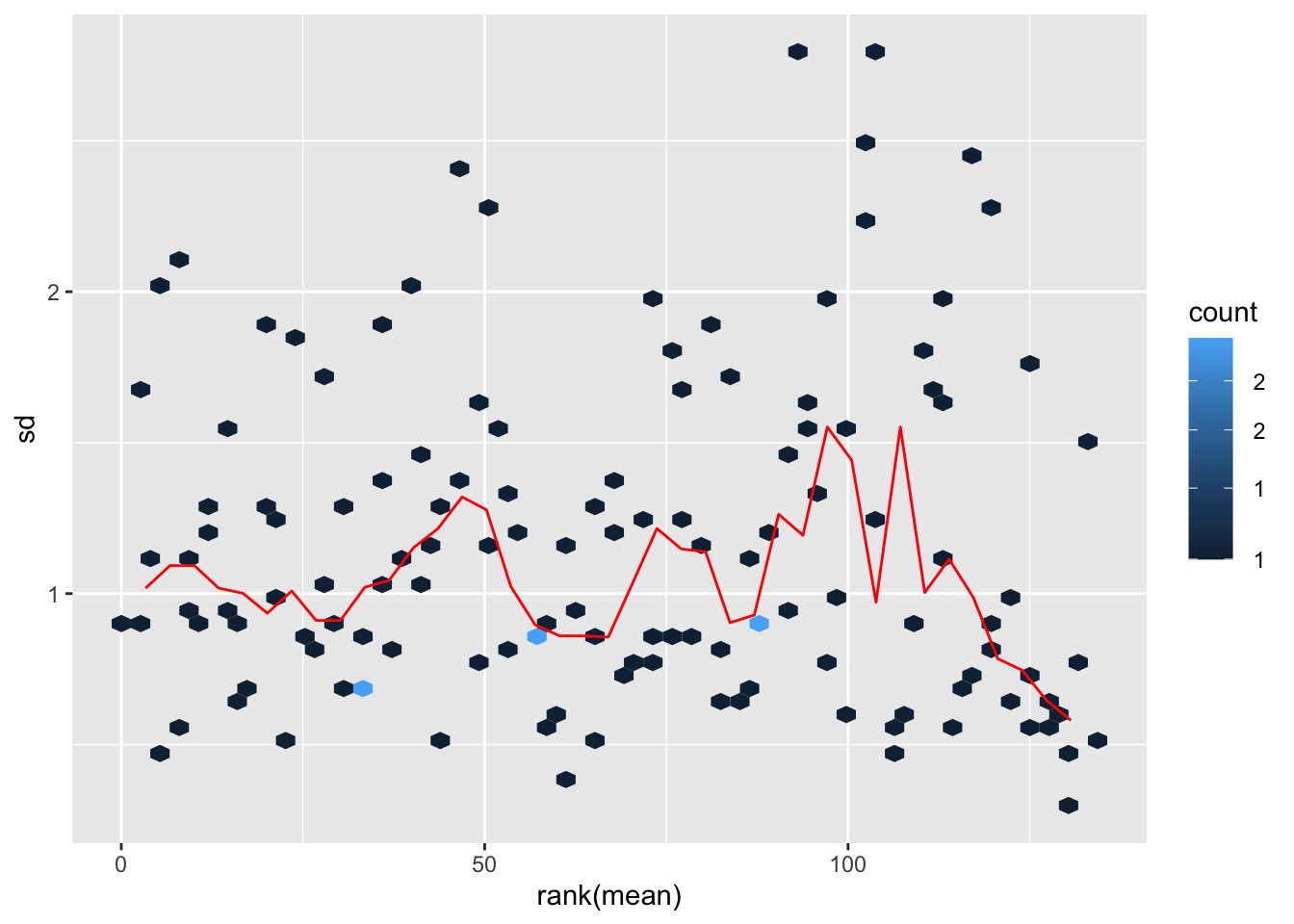
Imputation
metaImp.MinDet <- DEP::impute(metaNorm, "MinDet")
metaImp.zero <- DEP::impute(metaNorm, "zero")
metaImp.bpca<- DEP::impute(metaNorm, "bpca")
assays(metaFilt)[["norm"]] <- normMat
assays(metaFilt)[["imputed"]] <- assay(metaImp.MinDet)
assays(metaFilt)[["imputed.bpca"]] <- assay(metaImp.bpca)
assays(metaFilt)[["imputed.zero"]] <- assay(metaImp.zero)
Distribution after imputation
countMat <- assays(metaFilt)[["imputed.bpca"]]
countTab <- countMat %>% as_tibble(rownames = "id") %>%
    pivot_longer(-id) %>%
    filter(!is.na(value))
ggplot(countTab, aes(x=name, y=value)) +
    geom_boxplot() + geom_point()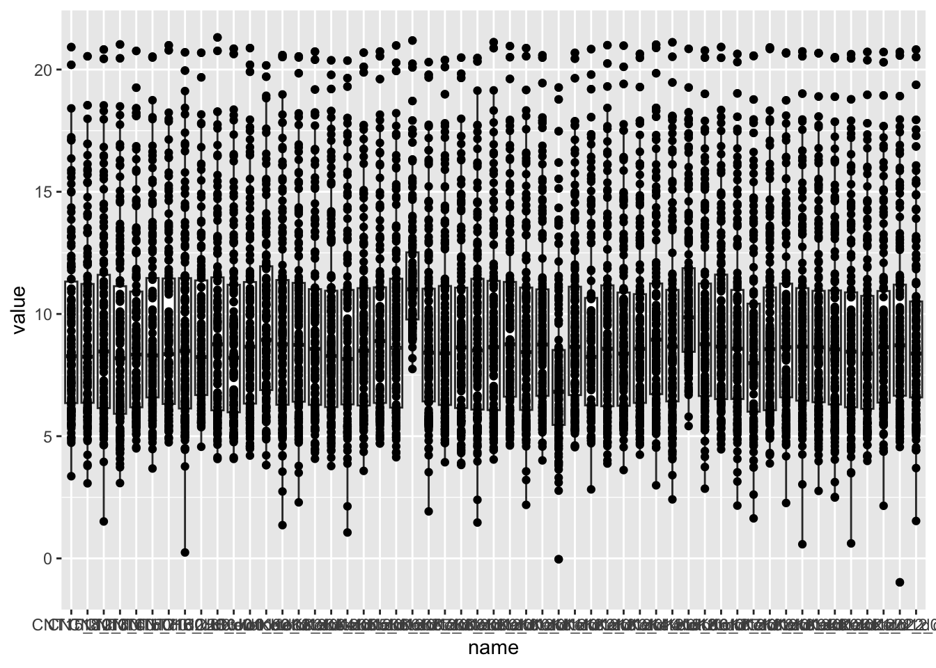
Heatmap visualization
library(pheatmap)
#select top 1000 most variant
colAnno <- colData(metaFilt) %>% data.frame()
colAnno <- colAnno[,c("time","group")]
#colAnno[["sampleName"]] <- NULL
plotMat <- assays(metaFilt)[["imputed.bpca"]]
plotMat <- jyluMisc::mscale(plotMat, center = TRUE, scale = TRUE, censor = 4)
pheatmap(plotMat, show_rownames = FALSE, scale = "none",
         annotation_col = colAnno,
         clustering_method = "ward.D2")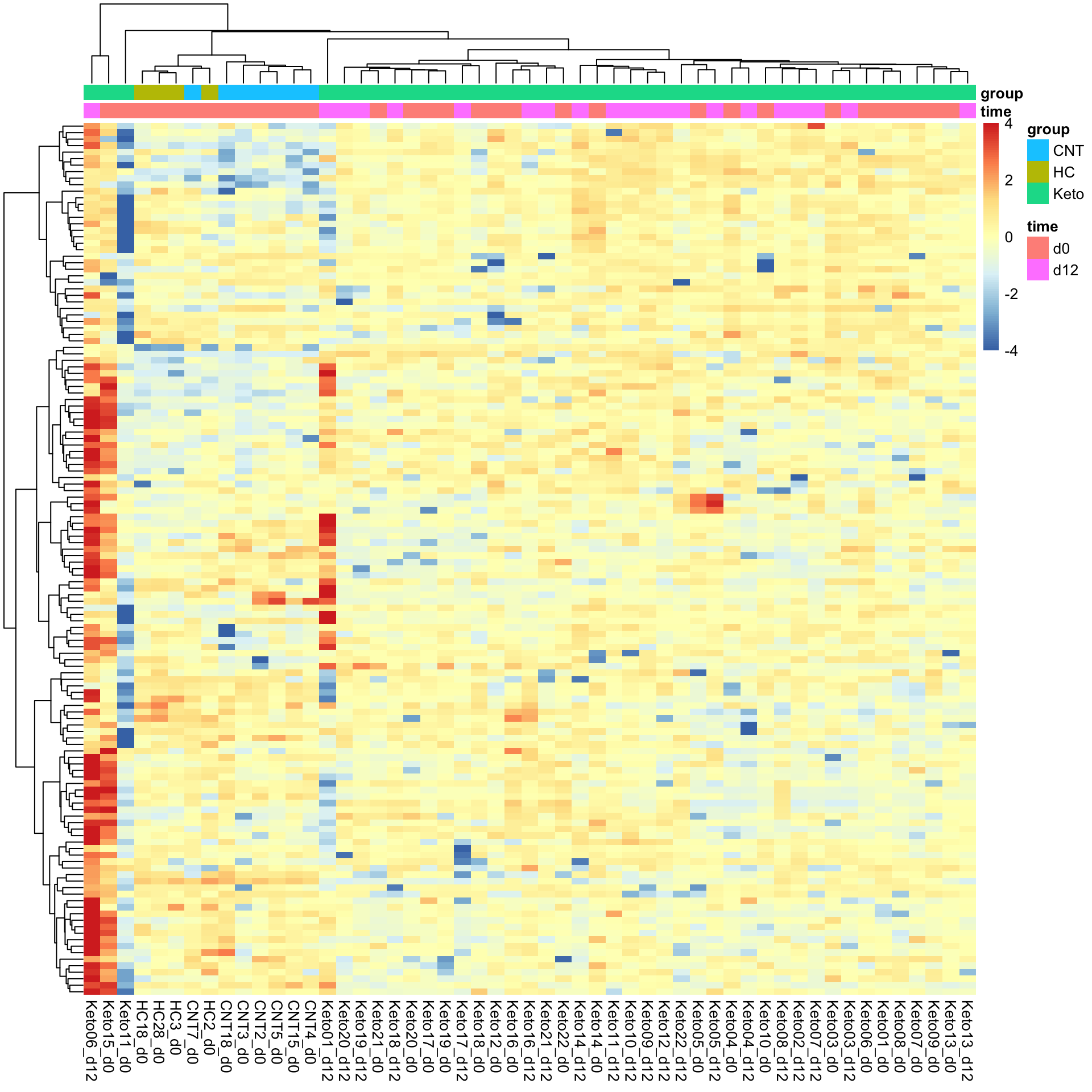
PCA
plotMat  <- assays(metaFilt)[["imputed.bpca"]]
prRes <- prcomp(t(plotMat), scale. = FALSE, center = TRUE)
plotTab <- prRes$x %>% as_tibble(rownames = "sampleID") %>%
    left_join(as_tibble(colAnno, rownames = "sampleID"))
ggplot(plotTab, aes(x=PC1, y=PC2, col = group)) +
    geom_point() +
    ggrepel::geom_text_repel(aes(label = sampleID))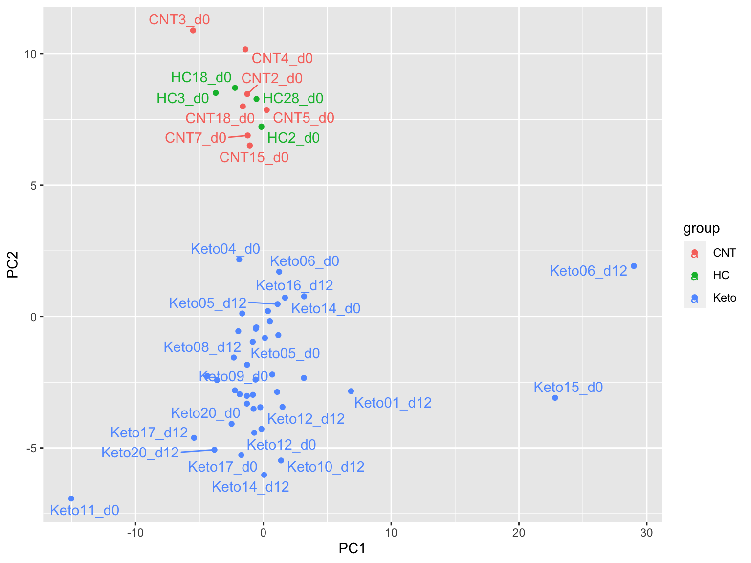
prRes <- prcomp(t(plotMat), scale. = FALSE, center = FALSE)
plotTab <- prRes$x %>% as_tibble(rownames = "sampleID") %>%
    left_join(as_tibble(colAnno, rownames = "sampleID"))
ggplot(plotTab, aes(x=PC3, y=PC4, col = group)) +
    geom_point() +
    ggrepel::geom_text_repel(aes(label = sampleID))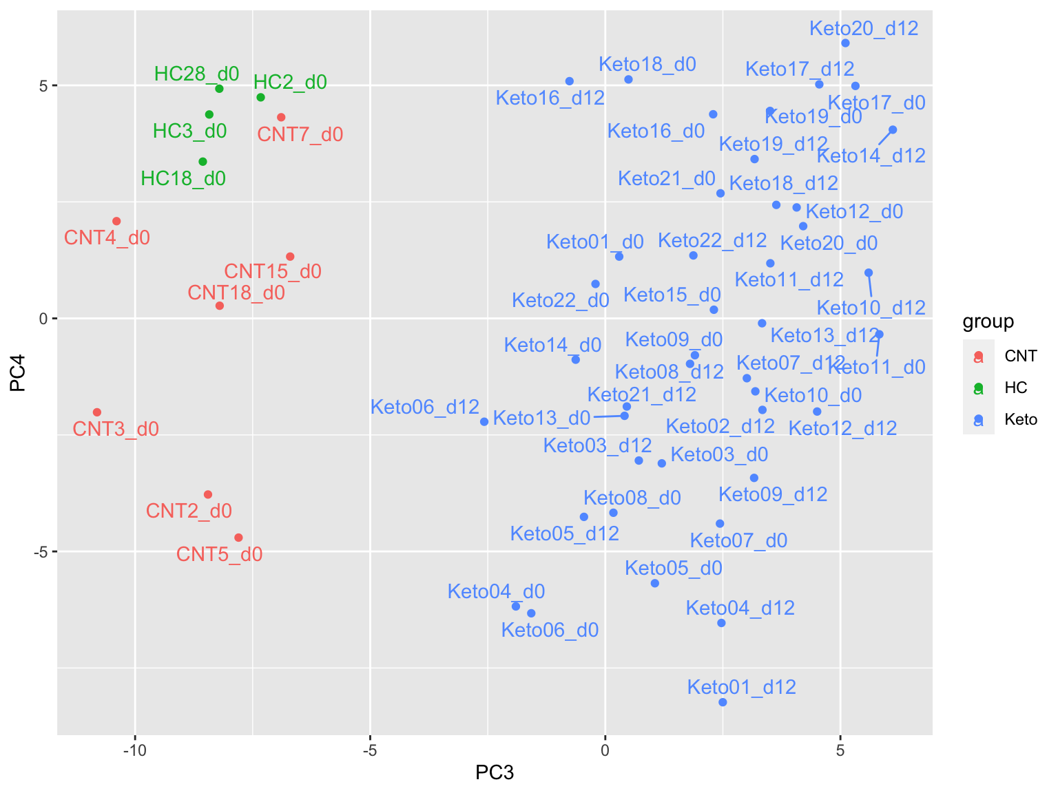
Analysis focused on keto group
metaKeto <- metaFilt[,metaFilt$group == "Keto"]Heatmap visualization
library(pheatmap)
#select top 1000 most variant
colAnno <- colData(metaKeto) %>% data.frame()
colAnno <- colAnno[,c("time","group")]
#colAnno[["sampleName"]] <- NULL
plotMat <- assays(metaKeto)[["imputed.bpca"]]
plotMat <- jyluMisc::mscale(plotMat, center = TRUE, scale = TRUE, censor = 4)
pheatmap(plotMat, show_rownames = FALSE, scale = "none",
         annotation_col = colAnno,
         clustering_method = "ward.D2")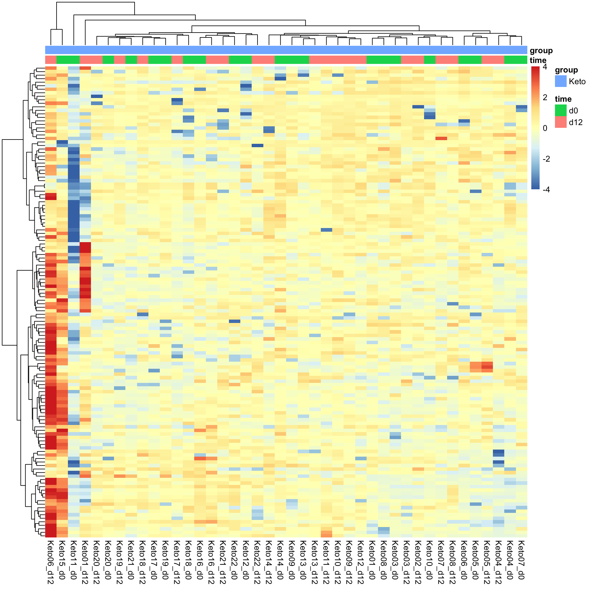
PCA
plotMat <- assays(metaKeto)[["imputed.bpca"]]
prRes <- prcomp(t(plotMat), scale. = FALSE, center = TRUE)
plotTab <- prRes$x %>% as_tibble(rownames = "sampleID") %>%
    left_join(as_tibble(colAnno, rownames = "sampleID"))
ggplot(plotTab, aes(x=PC1, y=PC2, col = time)) +
    geom_point() +
    ggrepel::geom_text_repel(aes(label = sampleID))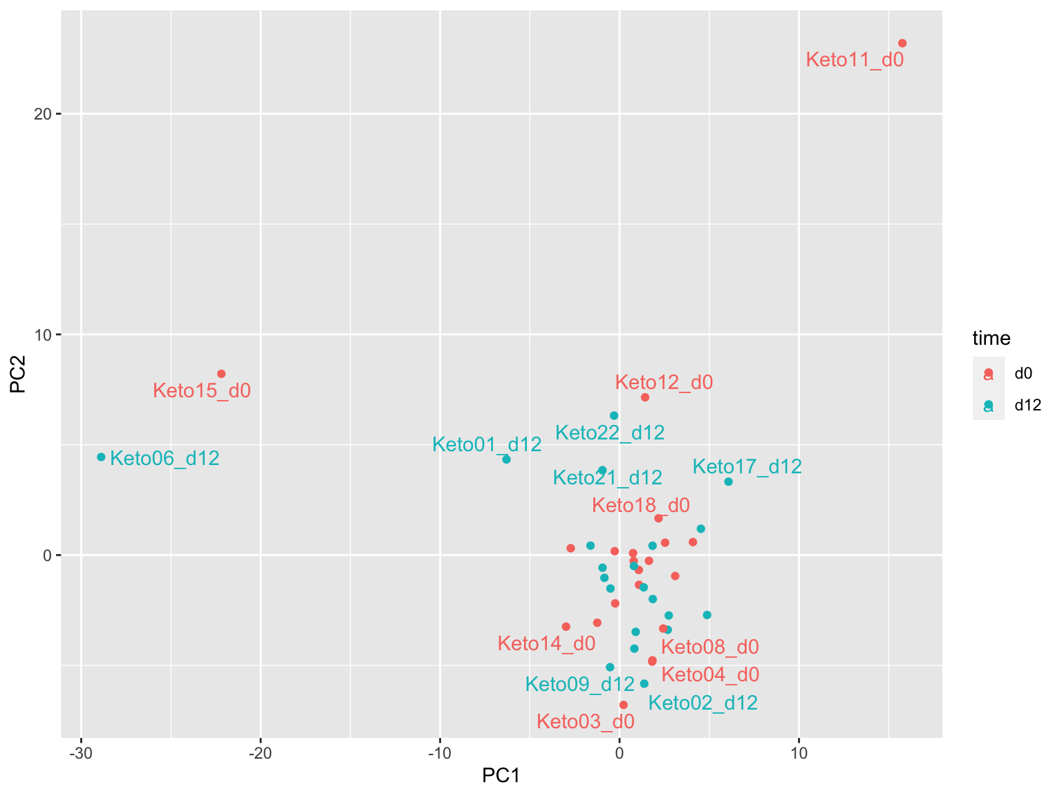
prRes <- prcomp(t(plotMat), scale. = FALSE, center = FALSE)
plotTab <- prRes$x %>% as_tibble(rownames = "sampleID") %>%
    left_join(as_tibble(colAnno, rownames = "sampleID"))
ggplot(plotTab, aes(x=PC3, y=PC4, col = time)) +
    geom_point() +
    ggrepel::geom_text_repel(aes(label = sampleID))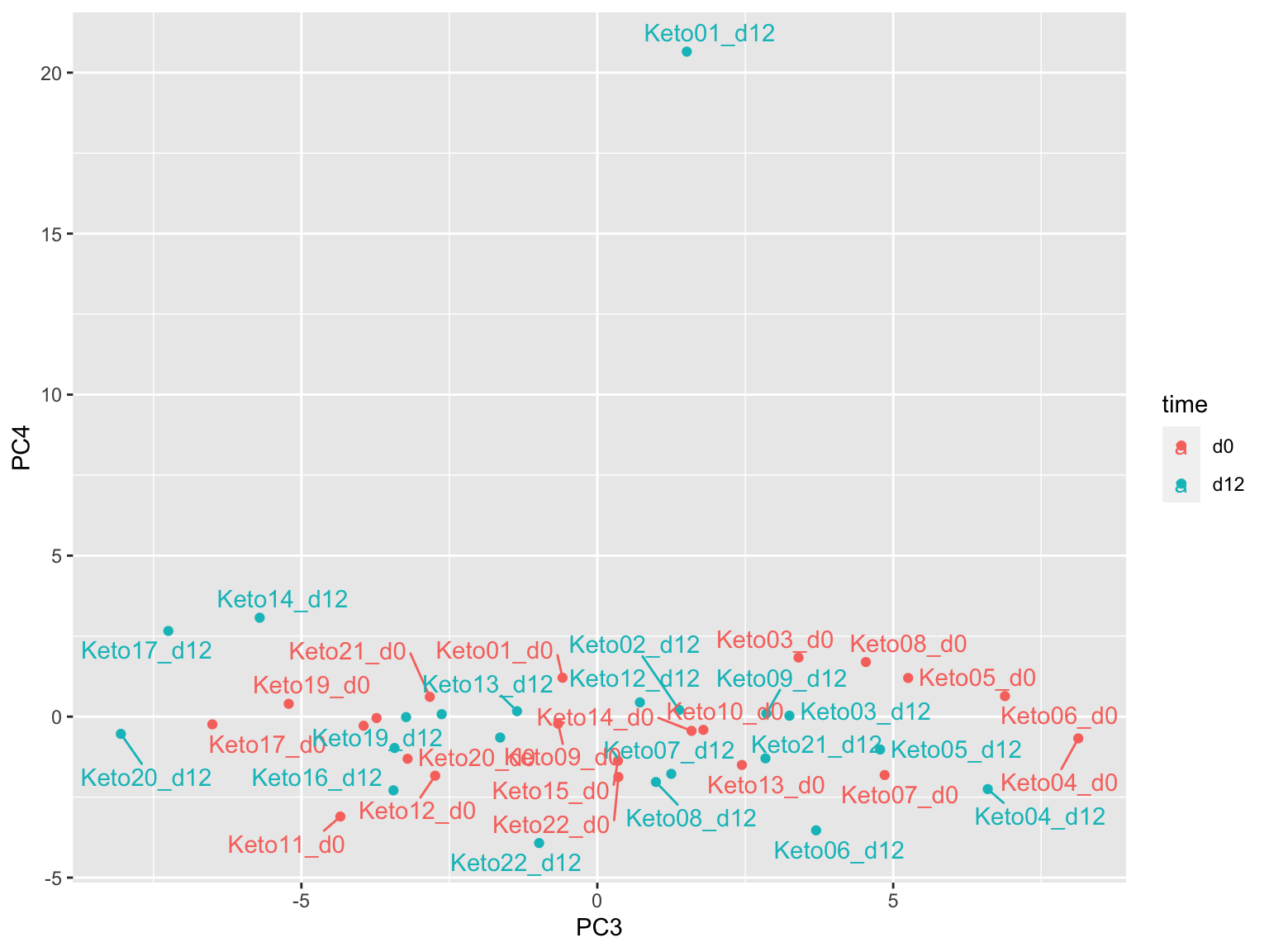
Identify change between d12 and d0
library(proDA)
metaMat <- assays(metaKeto)[["norm"]]
designMat <- model.matrix(~patID + time, colData(metaKeto))

fit <- proDA(metaMat, design = designMat)

resTab <- test_diff(fit, contrast = "timed12") %>%
  arrange(pval) %>%
  mutate(metabolite = rowData(seMeta)[name,]$name)
hist(resTab$pval)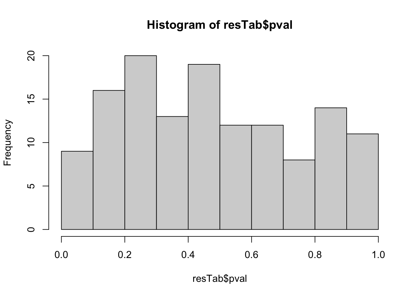 Not strong difference
metabolites with p-value < 0.1
resTab.sig <- filter(resTab, pval < 0.1)
resTab.sig %>% select(metabolite, pval, adj_pval, diff) %>%
  mutate_if(is.numeric, formatC, digits=1) %>%
  DT::datatable()
Plot
pList <- lapply(seq(nrow(resTab.sig)), function(i) {
  rec <- resTab.sig[i,]
  plotTab <- tibble(abundance = metaMat[rec$name,],
                    time = metaKeto$time,
                    patID = metaKeto$patID)
  ggplot(plotTab, aes(x=time, y=abundance)) +
    geom_point(aes(col = time)) +
    geom_line(aes(group = patID), linetype = "dashed") +
    ggtitle(sprintf("%s (p=%1.2f)", rec$metabolite, rec$pval)) +
    theme_bw()
})

cowplot::plot_grid(plotlist = pList,ncol=2)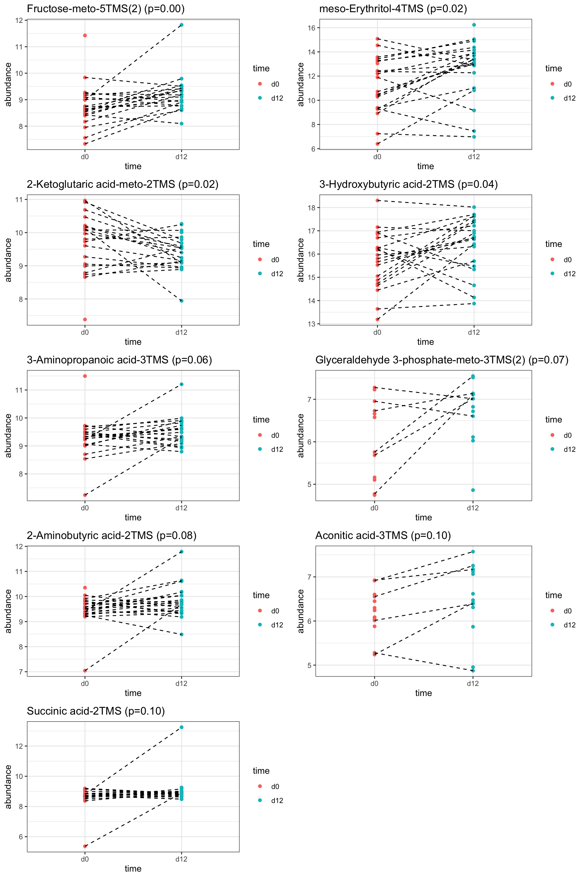
Identify change between d12 and d0, try removing two potential outlier patient, Keto06 and Keto15
library(proDA)
metaKeto <- metaKeto[,!metaKeto$patID %in% c("Keto06","Keto15")]
metaMat <- assays(metaKeto)[["norm"]]
designMat <- model.matrix(~patID + time, colData(metaKeto))

fit <- proDA(metaMat, design = designMat)

resTab <- test_diff(fit, contrast = "timed12") %>%
  arrange(pval) %>%
  mutate(metabolite = rowData(seMeta)[name,]$name)
hist(resTab$pval)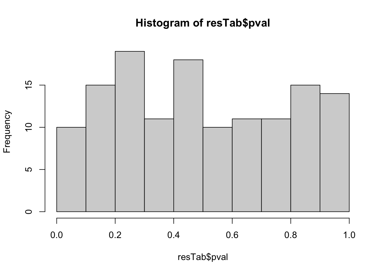 Not strong difference
metabolites with p-value < 0.1
resTab.sig <- filter(resTab, pval < 0.1)
resTab.sig %>% select(metabolite, pval, adj_pval, diff) %>%
  mutate_if(is.numeric, formatC, digits=1) %>%
  DT::datatable()
Plot
pList <- lapply(seq(nrow(resTab.sig)), function(i) {
  rec <- resTab.sig[i,]
  plotTab <- tibble(abundance = metaMat[rec$name,],
                    time = metaKeto$time,
                    patID = metaKeto$patID)
  ggplot(plotTab, aes(x=time, y=abundance)) +
    geom_point(aes(col = time)) +
    geom_line(aes(group = patID), linetype = "dashed") +
    ggtitle(sprintf("%s (p=%1.2f)", rec$metabolite, rec$pval)) +
    theme_bw()
})

cowplot::plot_grid(plotlist = pList,ncol=2)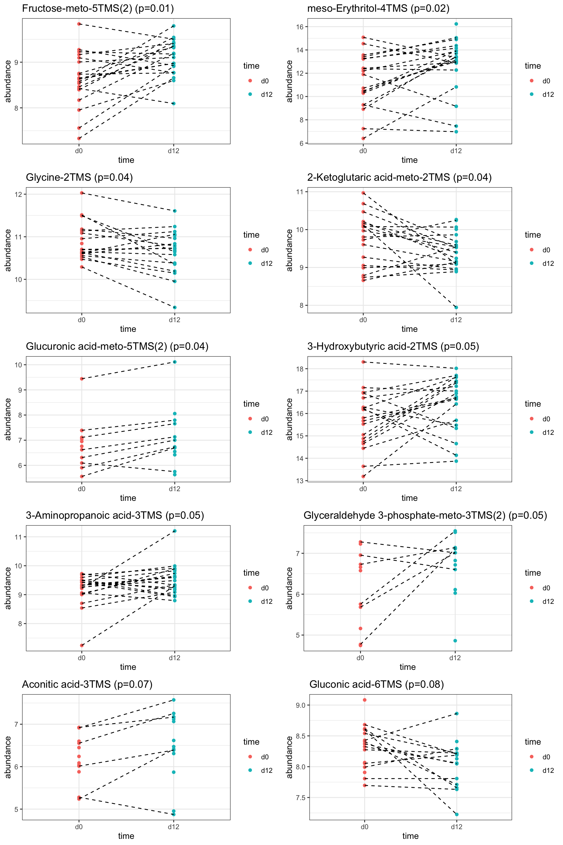
sessionInfo()R version 4.2.0 (2022-04-22)
Platform: x86_64-apple-darwin17.0 (64-bit)
Running under: macOS Big Sur/Monterey 10.16
Matrix products: default
BLAS: /Library/Frameworks/R.framework/Versions/4.2/Resources/lib/libRblas.0.dylib
LAPACK: /Library/Frameworks/R.framework/Versions/4.2/Resources/lib/libRlapack.dylib
locale:
[1] en_US.UTF-8/en_US.UTF-8/en_US.UTF-8/C/en_US.UTF-8/en_US.UTF-8
attached base packages:
[1] stats4 stats graphics grDevices utils datasets methods
[8] base
other attached packages:
[1] proDA_1.10.0 pheatmap_1.0.12
[3] forcats_0.5.1 stringr_1.4.1
[5] dplyr_1.1.4.9000 purrr_0.3.4
[7] readr_2.1.2 tidyr_1.2.0
[9] tibble_3.2.1 ggplot2_3.4.1
[11] tidyverse_1.3.2 SummarizedExperiment_1.26.1
[13] GenomicRanges_1.48.0 GenomeInfoDb_1.32.2
[15] IRanges_2.30.0 S4Vectors_0.34.0
[17] MatrixGenerics_1.8.1 matrixStats_0.62.0
[19] jyluMisc_0.1.5 vsn_3.64.0
[21] Biobase_2.56.0 BiocGenerics_0.42.0
loaded via a namespace (and not attached):
[1] DEP_1.18.0 utf8_1.2.4 shinydashboard_0.7.2
[4] gmm_1.6-6 tidyselect_1.2.1 htmlwidgets_1.5.4
[7] grid_4.2.0 BiocParallel_1.30.3 norm_1.0-10.0
[10] maxstat_0.7-25 munsell_0.5.0 codetools_0.2-18
[13] preprocessCore_1.58.0 DT_0.23 withr_3.0.0
[16] colorspace_2.0-3 highr_0.9 knitr_1.39
[19] rstudioapi_0.13 ggsignif_0.6.3 mzID_1.34.0
[22] labeling_0.4.2 git2r_0.30.1 slam_0.1-50
[25] GenomeInfoDbData_1.2.8 KMsurv_0.1-5 farver_2.1.1
[28] rprojroot_2.0.3 vctrs_0.6.5 generics_0.1.3
[31] TH.data_1.1-1 xfun_0.31 sets_1.0-21
[34] R6_2.5.1 doParallel_1.0.17 clue_0.3-61
[37] MsCoreUtils_1.8.0 bitops_1.0-7 cachem_1.0.6
[40] fgsea_1.22.0 DelayedArray_0.22.0 assertthat_0.2.1
[43] promises_1.2.0.1 scales_1.2.0 multcomp_1.4-19
[46] googlesheets4_1.0.0 gtable_0.3.0 extraDistr_1.9.1
[49] Cairo_1.6-0 affy_1.74.0 sandwich_3.0-2
[52] workflowr_1.7.0 rlang_1.1.3 mzR_2.30.0
[55] GlobalOptions_0.1.2 splines_4.2.0 rstatix_0.7.0
[58] gargle_1.2.0 impute_1.70.0 hexbin_1.28.2
[61] broom_1.0.0 BiocManager_1.30.18 yaml_2.3.5
[64] abind_1.4-5 modelr_0.1.8 crosstalk_1.2.0
[67] backports_1.4.1 httpuv_1.6.6 tools_4.2.0
[70] relations_0.6-12 affyio_1.66.0 ellipsis_0.3.2
[73] gplots_3.1.3 jquerylib_0.1.4 RColorBrewer_1.1-3
[76] MSnbase_2.22.0 plyr_1.8.7 Rcpp_1.0.9
[79] visNetwork_2.1.0 zlibbioc_1.42.0 RCurl_1.98-1.7
[82] ggpubr_0.4.0 GetoptLong_1.0.5 cowplot_1.1.1
[85] zoo_1.8-10 ggrepel_0.9.1 haven_2.5.0
[88] cluster_2.1.3 exactRankTests_0.8-35 fs_1.5.2
[91] magrittr_2.0.3 magick_2.7.3 data.table_1.14.8
[94] circlize_0.4.15 reprex_2.0.1 survminer_0.4.9
[97] pcaMethods_1.88.0 googledrive_2.0.0 mvtnorm_1.1-3
[100] ProtGenerics_1.28.0 hms_1.1.1 shinyjs_2.1.0
[103] mime_0.12 evaluate_0.15 xtable_1.8-4
[106] XML_3.99-0.10 readxl_1.4.0 gridExtra_2.3
[109] shape_1.4.6 compiler_4.2.0 KernSmooth_2.23-20
[112] ncdf4_1.19 crayon_1.5.2 htmltools_0.5.4
[115] later_1.3.0 tzdb_0.3.0 lubridate_1.8.0
[118] DBI_1.1.3 dbplyr_2.2.1 ComplexHeatmap_2.12.1
[121] tmvtnorm_1.5 MASS_7.3-58 Matrix_1.5-4
[124] car_3.1-0 cli_3.6.2 imputeLCMD_2.1
[127] marray_1.74.0 parallel_4.2.0 igraph_1.3.4
[130] pkgconfig_2.0.3 km.ci_0.5-6 piano_2.12.0
[133] MALDIquant_1.21 xml2_1.3.3 foreach_1.5.2
[136] bslib_0.4.1 XVector_0.36.0 drc_3.0-1
[139] rvest_1.0.2 digest_0.6.30 rmarkdown_2.14
[142] cellranger_1.1.0 fastmatch_1.1-3 survMisc_0.5.6
[145] shiny_1.7.4 gtools_3.9.3 rjson_0.2.21
[148] lifecycle_1.0.4 jsonlite_1.8.3 carData_3.0-5
[151] limma_3.52.2 fansi_1.0.6 pillar_1.9.0
[154] lattice_0.20-45 fastmap_1.1.0 httr_1.4.3
[157] plotrix_3.8-2 survival_3.4-0 glue_1.7.0
[160] png_0.1-7 iterators_1.0.14 stringi_1.7.8
[163] sass_0.4.2 caTools_1.18.2