Exploratory and Power Analysis of the RA metabolomic and proteomic data

workflowr

• Summary
• Checks
• Past versions

Last updated: 2023-03-15

Checks: 5 1

Knit directory: RA_Tcell_omics/analysis/

This reproducible R Markdown analysis was created with workflowr (version 1.7.0). The Checks tab describes the reproducibility checks that were applied when the results were created. The Past versions tab lists the development history.

---

Environment: empty

Great job! The global environment was empty. Objects defined in the global environment can affect the analysis in your R Markdown file in unknown ways. For reproduciblity it’s best to always run the code in an empty environment.

Seed: set.seed(20221110)

The command set.seed(20221110) was run prior to running the code in the R Markdown file. Setting a seed ensures that any results that rely on randomness, e.g. subsampling or permutations, are reproducible.

Session information: recorded

Great job! Recording the operating system, R version, and package versions is critical for reproducibility.

Cache: none

Nice! There were no cached chunks for this analysis, so you can be confident that you successfully produced the results during this run.

File paths: relative

Great job! Using relative paths to the files within your workflowr project makes it easier to run your code on other machines.

Repository version: no version control

Tracking code development and connecting the code version to the results is critical for reproducibility. To start using Git, open the Terminal and type git init in your project directory.

---

This project is not being versioned with Git. To obtain the full reproducibility benefits of using workflowr, please see ?wflow_start.

---

Load libraries

library(vsn)
library(pwr)
library(jyluMisc)
library(SummarizedExperiment)
library(tidyverse)
knitr::opts_chunk$set(warning = FALSE, message = FALSE)

Analysis of metabolimic data

Preprocessing

metaTab <- readxl::read_xlsx("../data/Metabolomics-Exvivo_CD8.xlsx") %>%
    pivot_longer(-c("Sample name","Group"), values_to = "value", names_to = "metabolite") %>%
    dplyr::rename(sampleName = `Sample name`)
metaMat <- metaTab %>% select(-Group) %>%
    pivot_wider(names_from = "sampleName", values_from = "value") %>%
    column_to_rownames("metabolite") %>%
    as.matrix()

Visualize overall data distribution

Per sample

ggplot(metaTab, aes(x=sampleName, y=value)) +
    geom_boxplot() + geom_point(aes(col = Group)) +
    theme(axis.text = element_text(angle = 90, hjust = 1, vjust = 0.5))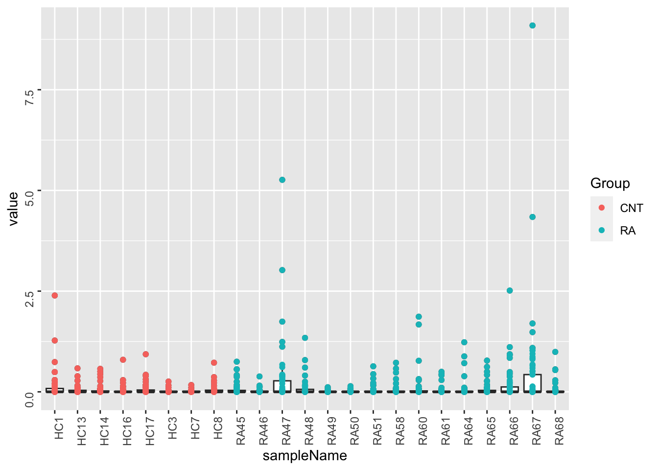

Per metabolite

ggplot(metaTab, aes(x=metabolite, y=value)) +
    geom_boxplot() + geom_point(aes(col = Group)) +
    theme(axis.text = element_text(angle = 90, hjust = 1, vjust = 0.5))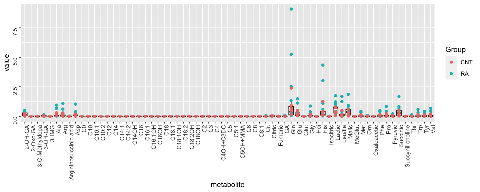

The abundance of different metabolites are very different. Transformation and Normalization may not be needed actually

PCA

pcRes <- prcomp(t(metaMat), scale. = TRUE, center = TRUE)$x
plotTab <- as_tibble(pcRes, rownames = "sampleName") %>%
    mutate(Group = metaTab[match(sampleName, metaTab$sampleName),]$Group)
ggplot(plotTab, aes(x=PC1, y=PC2, col = Group)) +
    geom_point()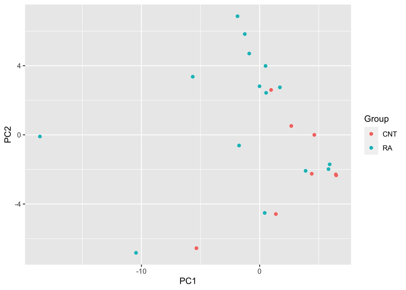

Differential abundance test

library(limma)
group <- factor(metaTab[match(colnames(metaMat), metaTab$sampleName),]$Group)
designMat <- model.matrix(~group)
lmFit <- lmFit(metaMat, design = designMat)
fit2 <- eBayes(lmFit)
resTab <- topTable(fit2, number = Inf) %>%
    as_tibble(rownames = "metabolite")
hist(resTab$P.Value)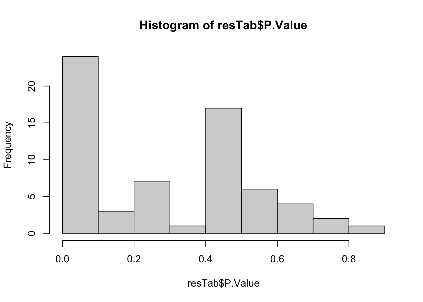

Plot significant associations

pList <- lapply(seq(nrow(filter(resTab, P.Value <= 0.05))), function(i) {
    rec <- resTab[i,]
    plotTab <- filter(metaTab, metabolite == rec$metabolite)
    ggplot(plotTab, aes(x=Group, y=value)) + 
        geom_boxplot(outlier.shape = NA) + 
        ggbeeswarm::geom_quasirandom(aes(color = Group), size=3) +
        ggtitle(sprintf("%s (P=%s)",rec$metabolite,formatC(rec$P.Value,digits = 2))) +
        theme_bw() +
        theme(legend.position = "none")
})
cowplot::plot_grid(plotlist = pList,ncol=3)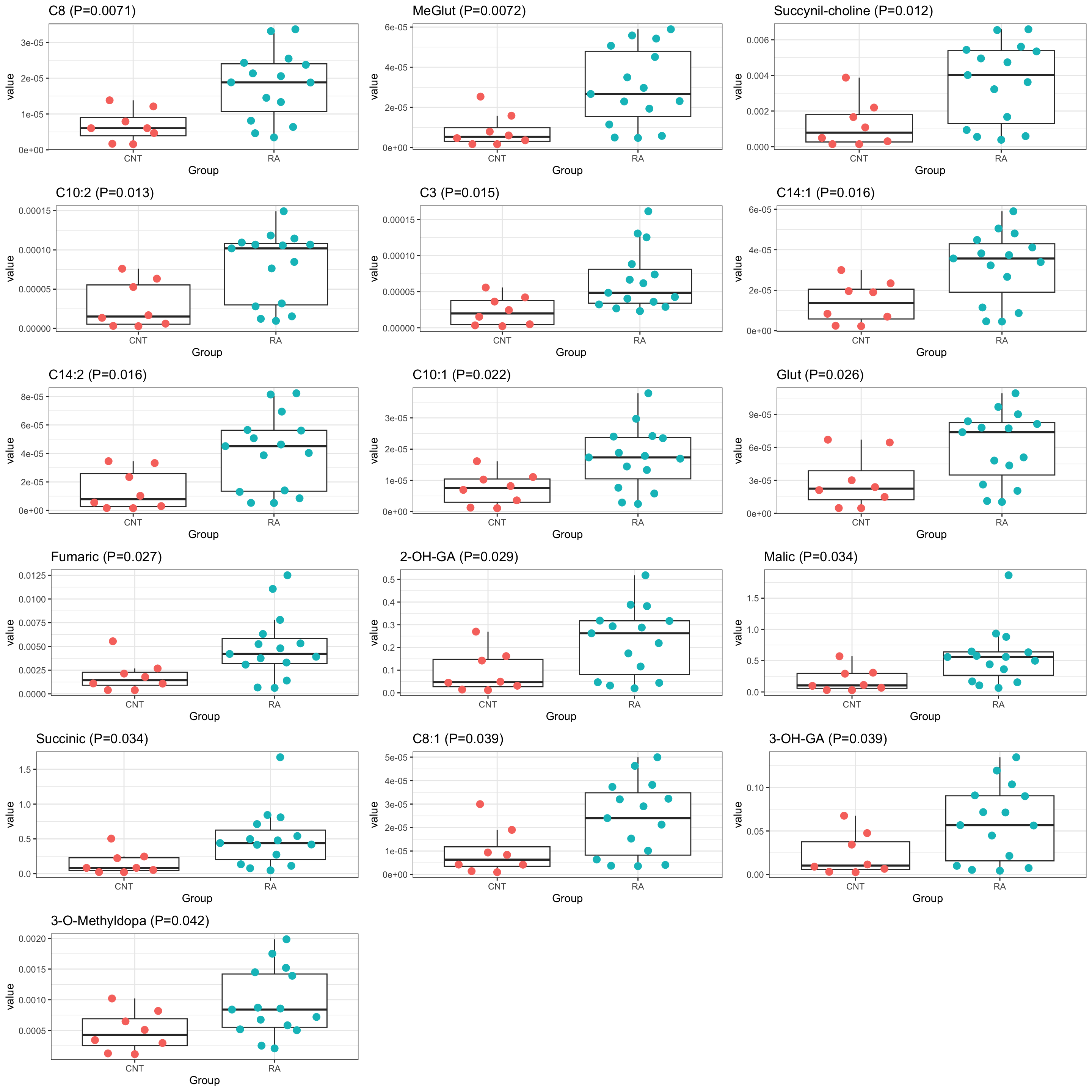

Power analysis to estimate sample size

meanTab <- metaTab %>%
    group_by(Group, metabolite) %>%
    summarise(mean = mean(value)) %>%
    pivot_wider(names_from = Group, values_from = mean)

sdTab <- metaTab %>%
    group_by(metabolite) %>%
    summarise(sd = sd(value))

dTab <- left_join(meanTab, sdTab) %>%
    mutate(d= abs(RA-CNT)/sd)

nTab <- lapply(seq(nrow(dTab)), function(i) {
    rec <- dTab[i,]
    n1 <- pwr.t.test(d = rec$d , sig.level = 0.05, 
                    power = 0.9, alternative = "two.sided")$n
    n2 <- pwr.t.test(d = rec$d , sig.level = 0.01, 
                    power = 0.9, alternative = "two.sided")$n
    tibble(metabolite = rec$metabolite, 
           n0.05 = as.integer(n1), n0.01=as.integer(n2))
}) %>% bind_rows() %>% 
    arrange(n0.05)

Table of sample number at certain p-value threshold

nTab %>%  DT::datatable()

Bar-plot

plotTab <- nTab %>% mutate(metabolite = factor(metabolite, levels = metabolite)) %>%
    pivot_longer(-metabolite)
ggplot(plotTab, aes(x=metabolite, y=value, fill = name)) +
    geom_bar(stat = "identity", position = "dodge") +
    scale_color_discrete(name = "P-value cut",
                         labels = c("0.01","0.05")) +
    coord_cartesian(ylim=c(0,100)) +
    theme_bw() +
    theme(axis.text.x = element_text(angle = 90, hjust = 1, vjust = 0.5)) +
    ylab("samples required per group")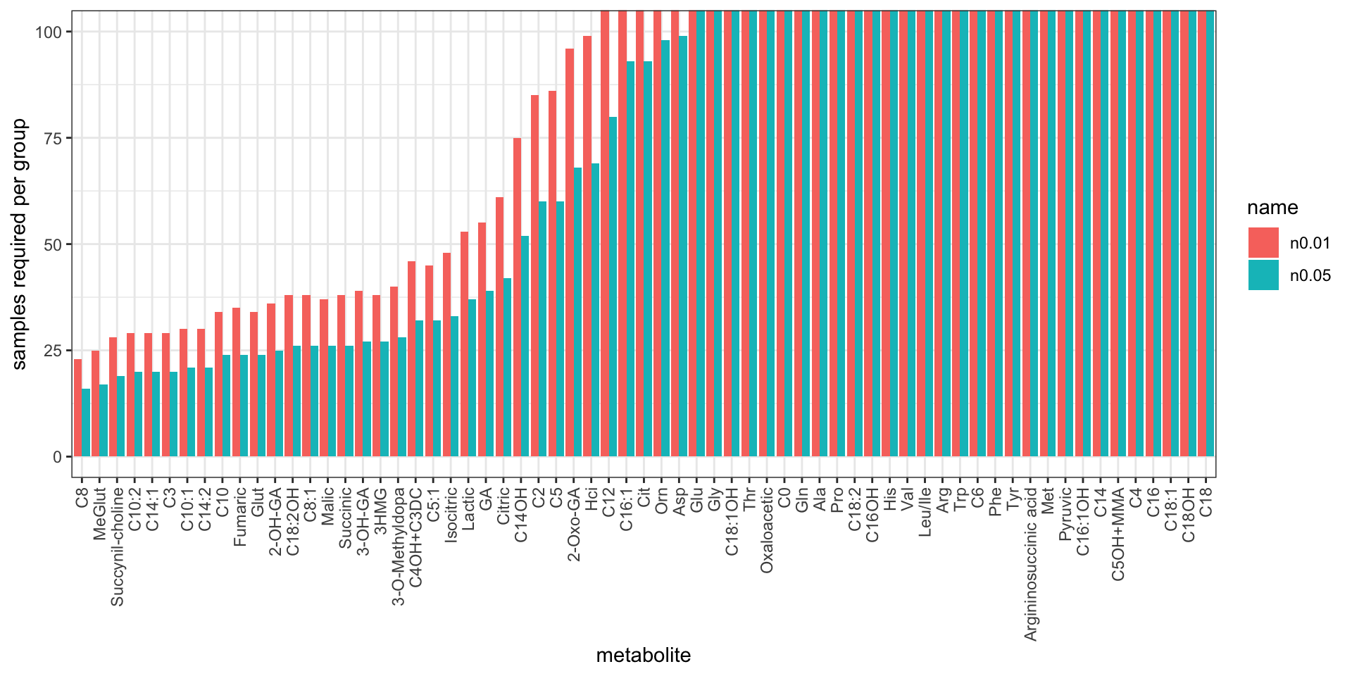

Analysis of the proteomic dataset

Data input

protData <- readxl::read_xlsx("../data/TF0489/TF0489_filtered_proteinGroups.xlsx") %>%
    select(`Majority protein IDs`, `Gene names`, contains("LFQ intensity")) %>%
    dplyr::rename(protID = `Majority protein IDs`, symbol = `Gene names`) %>%
    pivot_longer(-c("protID","symbol")) %>%
    mutate(name = str_remove(name,"LFQ intensity "))

Annotate samples

patAnno <- readxl::read_xlsx("../data/TF0489/Sample-Information.xlsx") %>%
    filter(!is.na(`Patient Group`))
patAnno <- patAnno[,c(1,2,4,5,6,7,8)]
colnames(patAnno) <- c("name","sampleName","Group","protConc","quantStart","sampleVol","bufferComp")
patAnno <- mutate(patAnno, name = paste0("Sample",sprintf("%02s",name)))

protData <- protData %>%
    left_join(patAnno, by = "name") %>%
    dplyr::rename(sampleID = name) %>%
    dplyr::rename(name = symbol) %>%
    mutate(ID = protID)

Check DNMT1 expression before any transformation

dnmtTab <- filter(protData, name == "DNMT1")
ggplot(dnmtTab, aes(x=Group, y=value)) +
    geom_boxplot() +
    geom_point()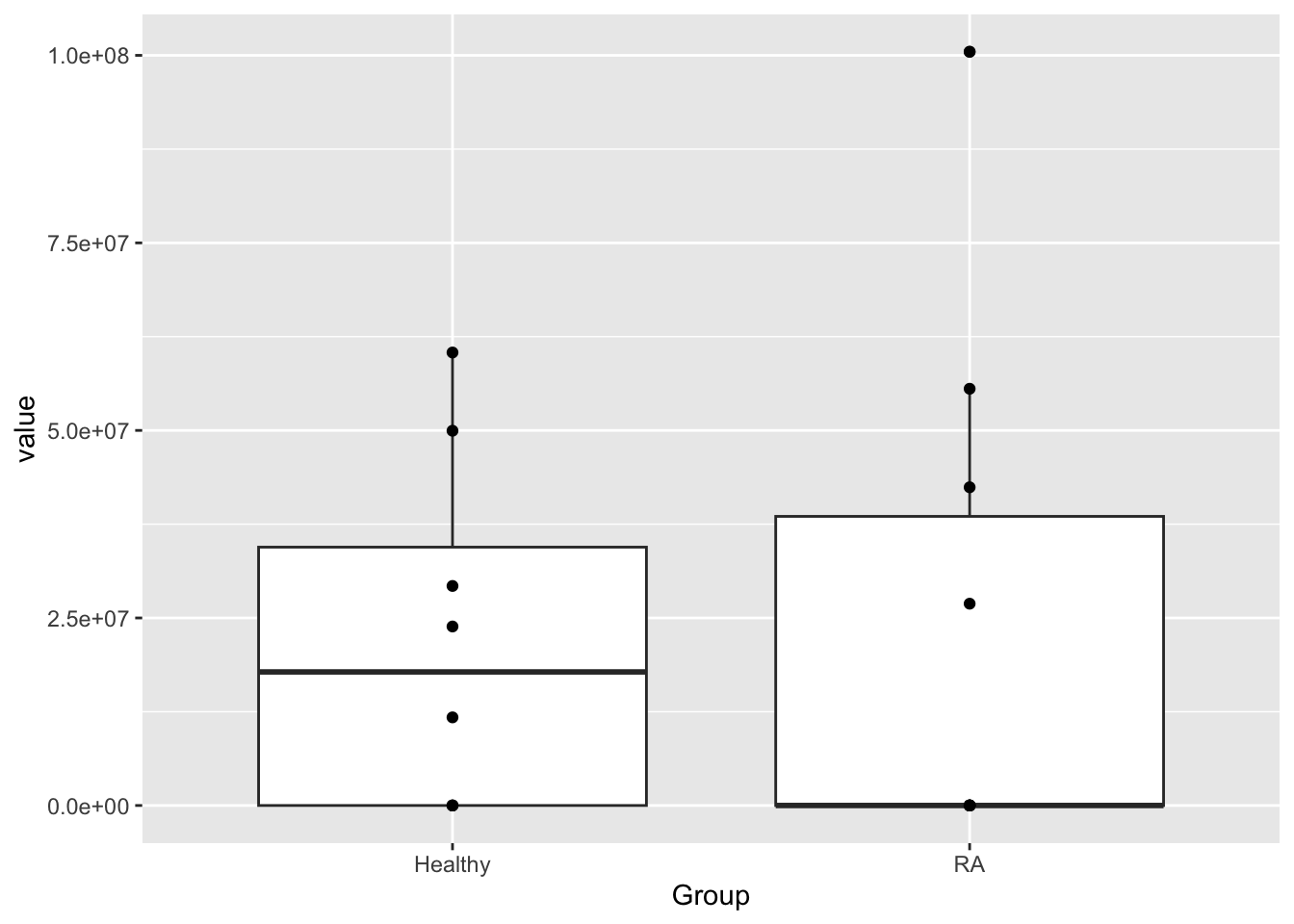

Remove undetected values

protData <- protData %>% filter(value >0)

Created summarised experiment

protObj <- jyluMisc::tidyToSum(protData, "protID", "sampleID","value",
                               annoRow = c("name","ID"),
                               annoCol = c("sampleName","Group",
                                           "protConc",
                                           "sampleVol","bufferComp"))

protMat <- assay(protObj)

boxplot(protMat)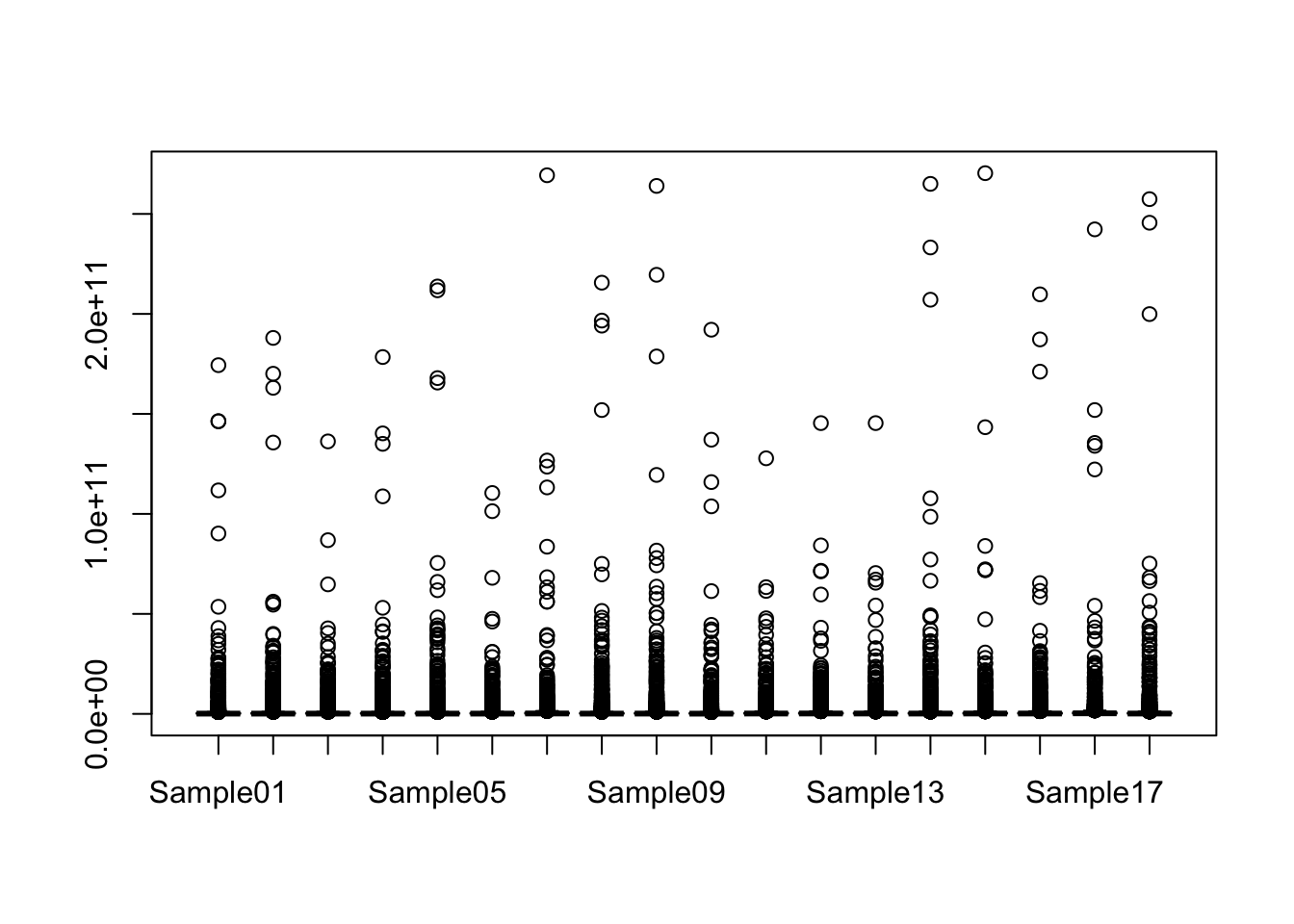

Needs proprocessing

Preprocess proteomic data

Missing value per sample

countMat <- assay(protObj)
plotTab <- tibble(sample = colnames(protObj), 
                  perNA = colSums(is.na(countMat))/nrow(countMat))
ggplot(plotTab, aes(x=sample, y=1-perNA)) +
    geom_bar(stat = "identity") +
    ylab("completeness") +
    theme(axis.text.x = element_text(angle = 90, hjust = 1, vjust=0))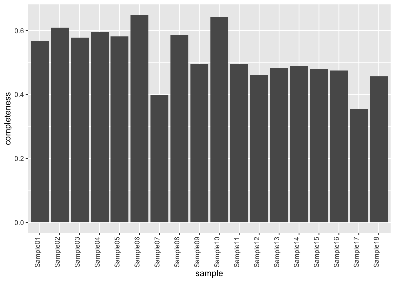

Plot a cumulative curve of missing value cut-off and remaining number of features

missRate <- tibble(id = rownames(countMat),
                   rate = rowSums(is.na(countMat))/ncol(countMat))
cumTab <- lapply(seq(0,1,0.05), function(cutRate) {
    tibble(cut= cutRate,
           per = sum(missRate$rate <= cutRate)/nrow(missRate))
} ) %>%
    bind_rows()
ggplot(cumTab, aes(x=cut,y=per)) +
    geom_line() +
    xlab("Allowed missing value rate") +
    ylab("Percentage of remaining features")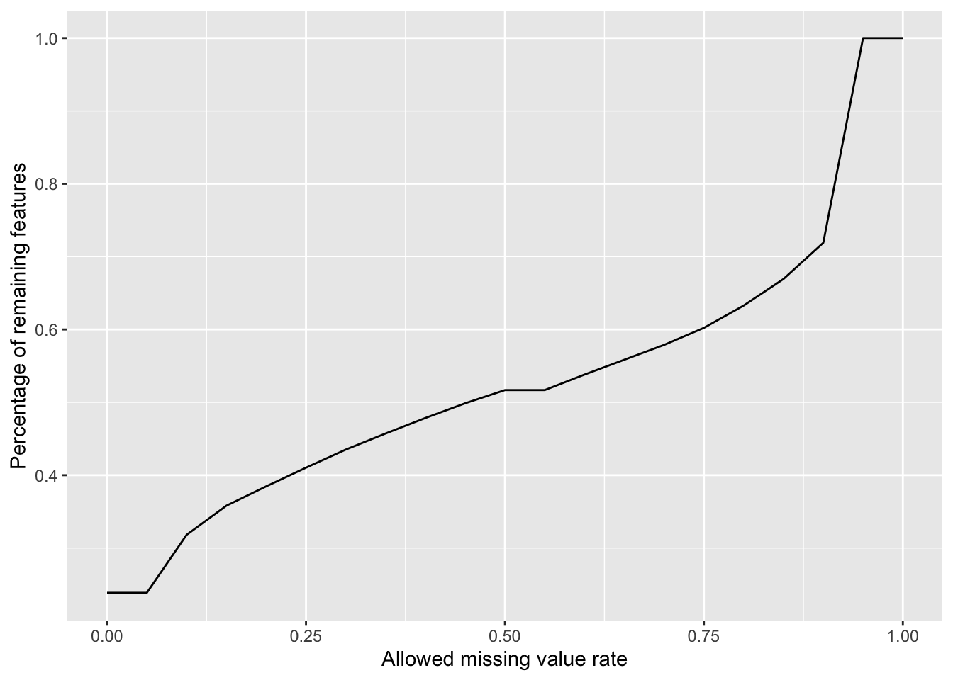

Missing value heatmap to check missing value structure

DEP::plot_missval(protObj)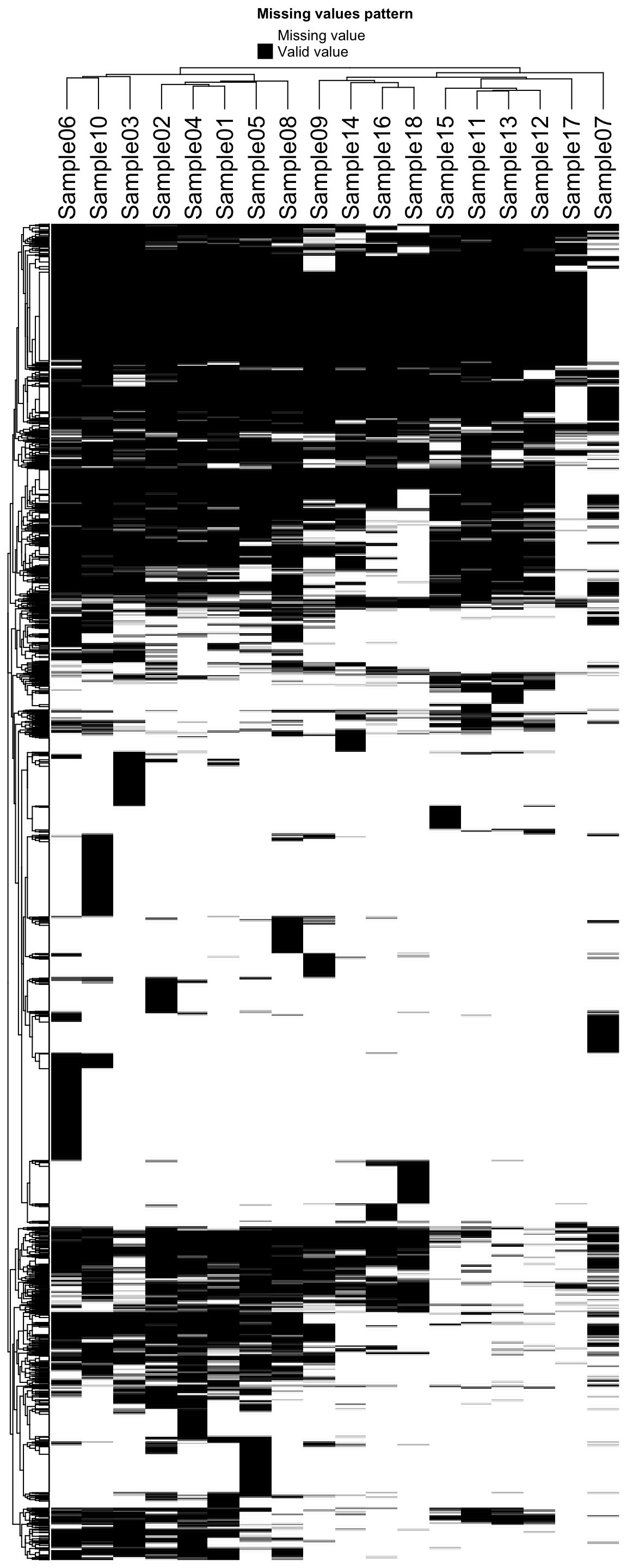

Rather random

Keep proteins detected in at least half of the sample (missing rate <= 0.5)

protFilt <- protObj[filter(missRate, rate <=0.5)$id,]
dim(protFilt)

[1] 2766   18

Data distribution

countMat <- assay(protFilt)
countTab <- countMat %>% as_tibble(rownames = "id") %>% 
    pivot_longer(-id) %>%
    filter(!is.na(value)) %>%
    mutate(log2Val = log2(value))

ggplot(countTab, aes(x=name, y=log2Val)) +
    geom_boxplot() + geom_point()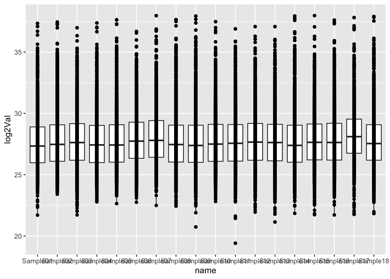

Imputation and normalization

Vst

protMat <- assay(protFilt)
fitVsn <- vsn::vsnMatrix(protMat)
normMat <- predict(fitVsn, newdata = protMat)
protNorm <- protFilt
assay(protNorm) <- normMat

Imputation

protImp <- DEP::impute(protNorm, "QRILC")
assays(protFilt)[["norm"]] <- normMat
assays(protFilt)[["imputed"]] <- assay(protImp)
rowData(protFilt) <- rowData(protImp)

Distribution after normalizaiton

countMat <- assays(protFilt)[["imputed"]]
countTab <- countMat %>% as_tibble(rownames = "id") %>% 
    pivot_longer(-id) %>%
    filter(!is.na(value))
ggplot(countTab, aes(x=name, y=value)) +
    geom_boxplot() + geom_point()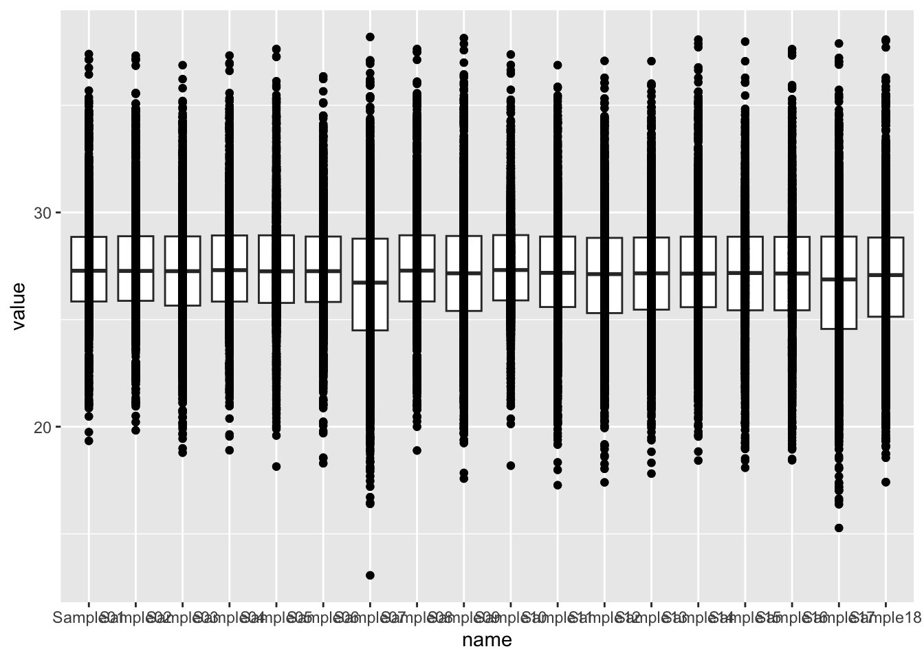

Mean versus variant plot

plotTab <- tibble(meanVal = rowMeans(countMat),
                  var = apply(countMat, 1, var))
ggplot(plotTab, aes(x=meanVal,y=var)) +
    geom_point()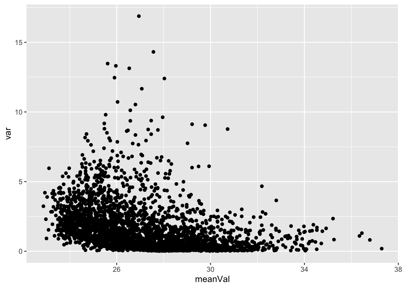

Heatmap visualization

library(pheatmap)
#select top 1000 most variant
colAnno <- colData(protFilt) %>% data.frame()
#colAnno[["sampleName"]] <- NULL
plotMat <- countMat[order(plotTab$var, decreasing = TRUE)[1:1000],]
pheatmap(plotMat, show_rownames = FALSE, scale = "row", 
         annotation_col = colAnno,
         clustering_method = "ward.D2")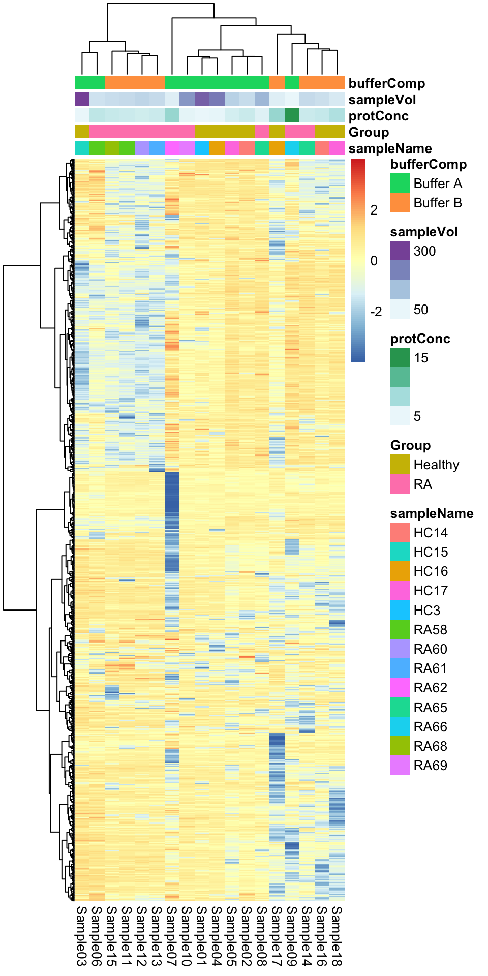

PCA

prRes <- prcomp(t(plotMat), scale. = TRUE, center = TRUE)
plotTab <- prRes$x %>% as_tibble(rownames = "sampleID") %>%
    left_join(as_tibble(colAnno, rownames = "sampleID"))
ggplot(plotTab, aes(x=PC1, y=PC2, col = Group, shape = bufferComp)) +
    geom_point() +
    ggrepel::geom_text_repel(aes(label = sampleName))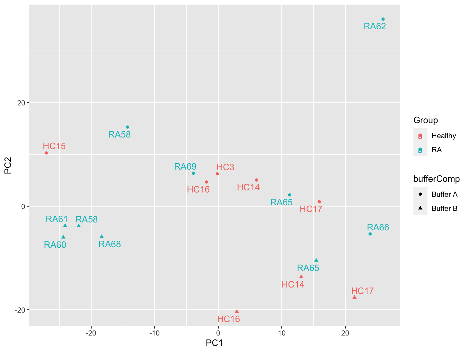

Buffer composition may act as a confounding factor. One sample, RA62 may be outlier.

Deal with technical replicates

Based on PCA, if there’s a replicate, choose buffer A

smpTab <- colData(protFilt) %>% as_tibble(rownames = "sampleID") %>%
    arrange(bufferComp, sampleName) %>% distinct(sampleName, .keep_all = TRUE)
protSub <- protFilt[,smpTab$sampleID]

Remove one potential outlier, RA62

protSub <- protSub[,protSub$sampleName != "RA62"]

Differential expression using proDA

protSub$Group <- factor(protSub$Group)
table(protSub$Group)

Healthy      RA 
      5       7 

Only keep proteins with symbols

protSub <- protSub[!rowData(protSub)$name %in% c("",NA),]

Differential protein expression using proDA

library(proDA)
protMat <- assays(protSub)[["norm"]]
fit <- proDA(protMat, design = ~ Group,
             col_data = colData(protSub))

resTab <- test_diff(fit, contrast = "GroupRA") %>%
  arrange(pval) %>%
  mutate(symbol = rowData(protSub[name,])$name)

hist(resTab$pval)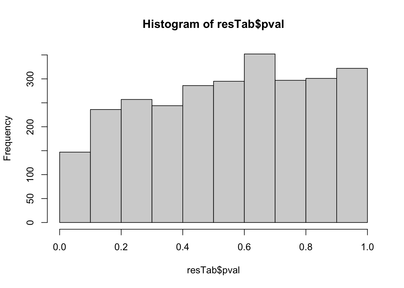

Not strong difference

Proteins with p-value < 0.05

resTab.sig <- filter(resTab, pval < 0.05)
resTab.sig %>% select(symbol, pval, adj_pval, diff) %>%
  mutate_if(is.numeric, formatC, digits=1) %>%
  DT::datatable()

Plot top 9 examples

pList <- lapply(seq(9), function(i) {
  rec <- resTab.sig[i,]
  plotTab <- tibble(expr = protMat[rec$name,],
                    Group = protSub$Group) 
  ggplot(plotTab, aes(x=Group, y=expr)) +
    geom_boxplot(outlier.shape = NA) +
    ggbeeswarm::geom_quasirandom(aes(color = Group), size=3) +
    ggtitle(rec$symbol) +
    theme_bw()
})

cowplot::plot_grid(plotlist = pList,ncol=3)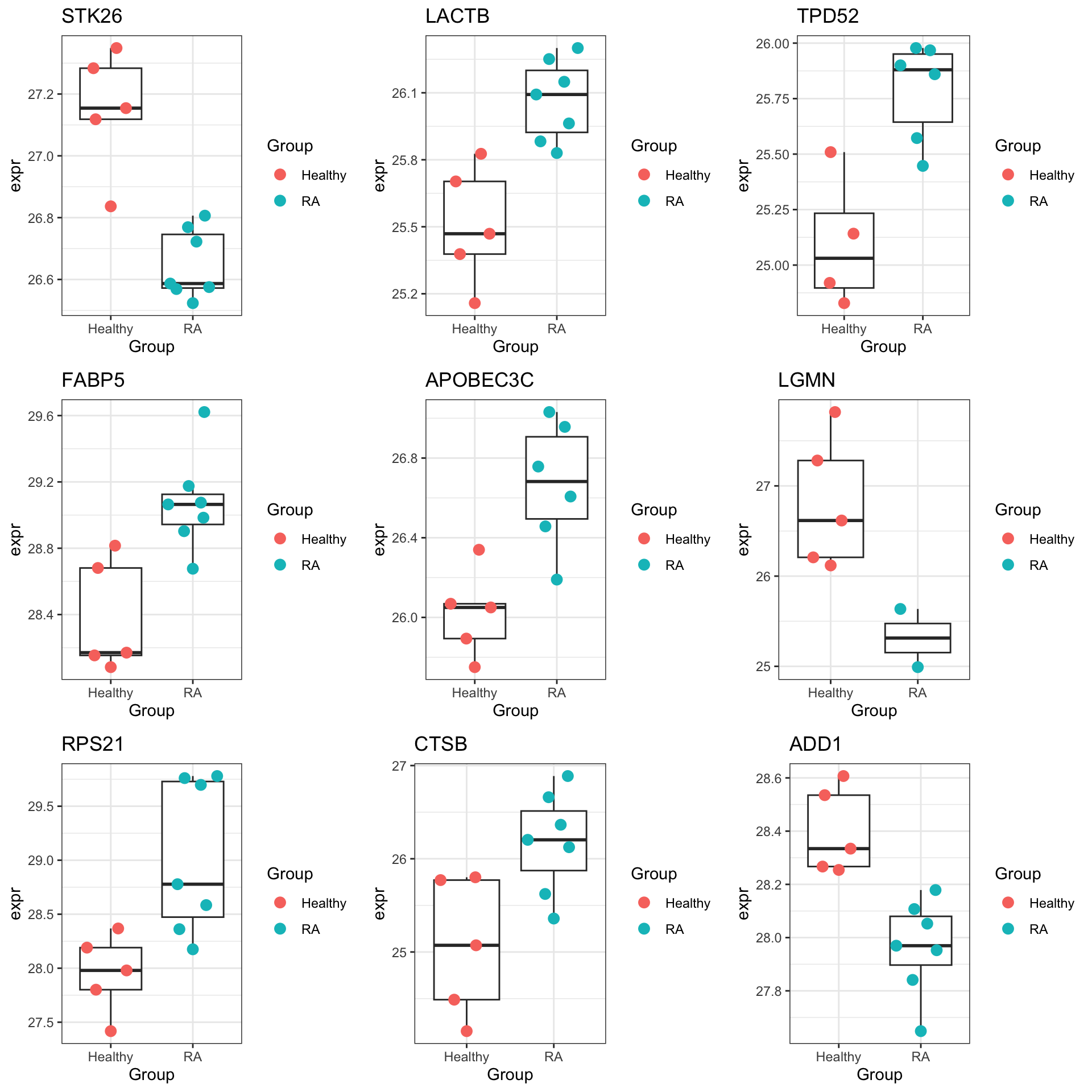

Enrichment analysis

gmts = list(H= "~/CLLproject_jlu/data/commonFiles/h.all.v6.2.symbols.gmt",
            KEGG = "~/CLLproject_jlu/data/commonFiles/c2.cp.kegg.v6.2.symbols.gmt",
            C6 = "~/CLLproject_jlu/data/commonFiles/c6.all.v6.2.symbols.gmt")
inputTab <- resTab %>% filter(pval < 0.1) %>%
  distinct(symbol, .keep_all = TRUE) %>%
  select(symbol, t_statistic) %>% data.frame() %>% column_to_rownames("symbol")
enRes <- list()
enRes[["Hallmark"]] <- runGSEA(inputTab, gmts$H, "page")
enRes[["KEGG"]] <- runGSEA(inputTab, gmts$KEGG,"page")
enRes[["Perturbation"]] <- runGSEA(inputTab, gmts$C6,"page")
p <- plotEnrichmentBar(enRes, pCut =0.05, ifFDR= FALSE)
cowplot::plot_grid(p)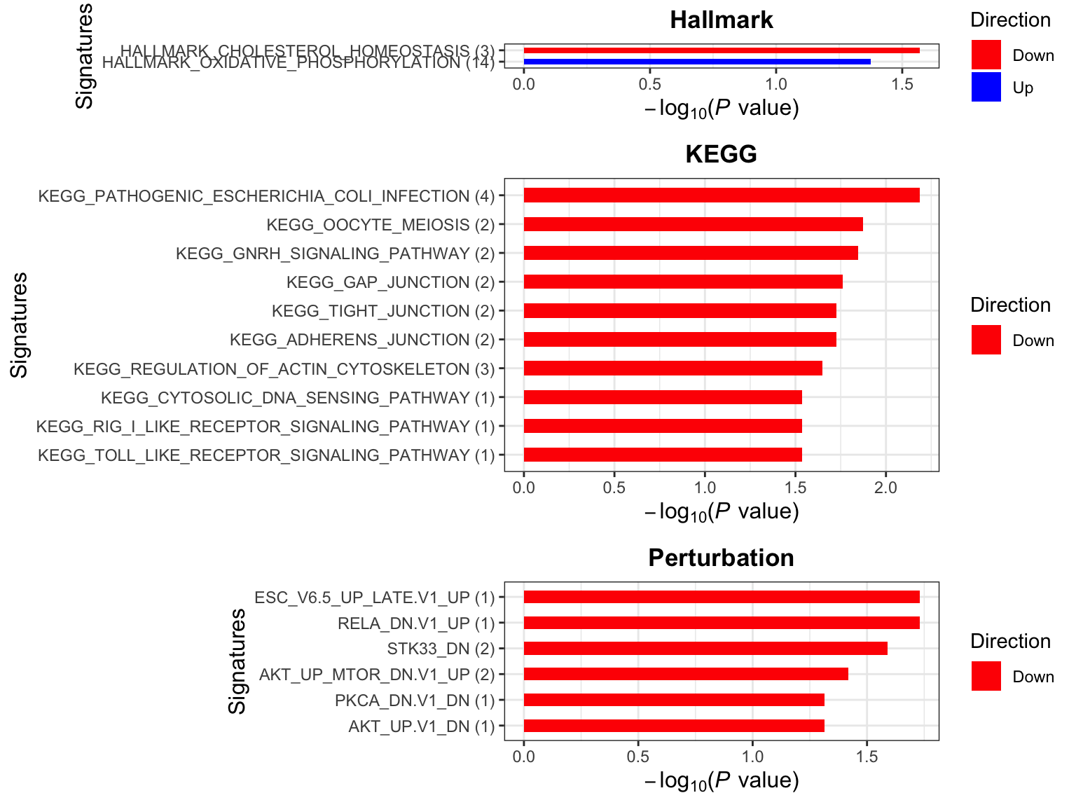

Plot expression of proteins from OXPHOS pathway

geneList <- piano::loadGSC(gmts$H)$gsc
resTab.oxphos <- filter(resTab, pval < 0.1, 
                        symbol %in% geneList$HALLMARK_OXIDATIVE_PHOSPHORYLATION)
pList <- lapply(seq(nrow(resTab.oxphos)), function(i) {
  rec <- resTab.oxphos[i,]
  plotTab <- tibble(expr = protMat[rec$name,],
                    Group = protSub$Group) 
  ggplot(plotTab, aes(x=Group, y=expr)) +
    geom_boxplot(outlier.shape = NA) +
    ggbeeswarm::geom_quasirandom(aes(color = Group), size=3) +
    ggtitle(rec$symbol) +
    theme_bw()
})

cowplot::plot_grid(plotlist = pList,ncol=3)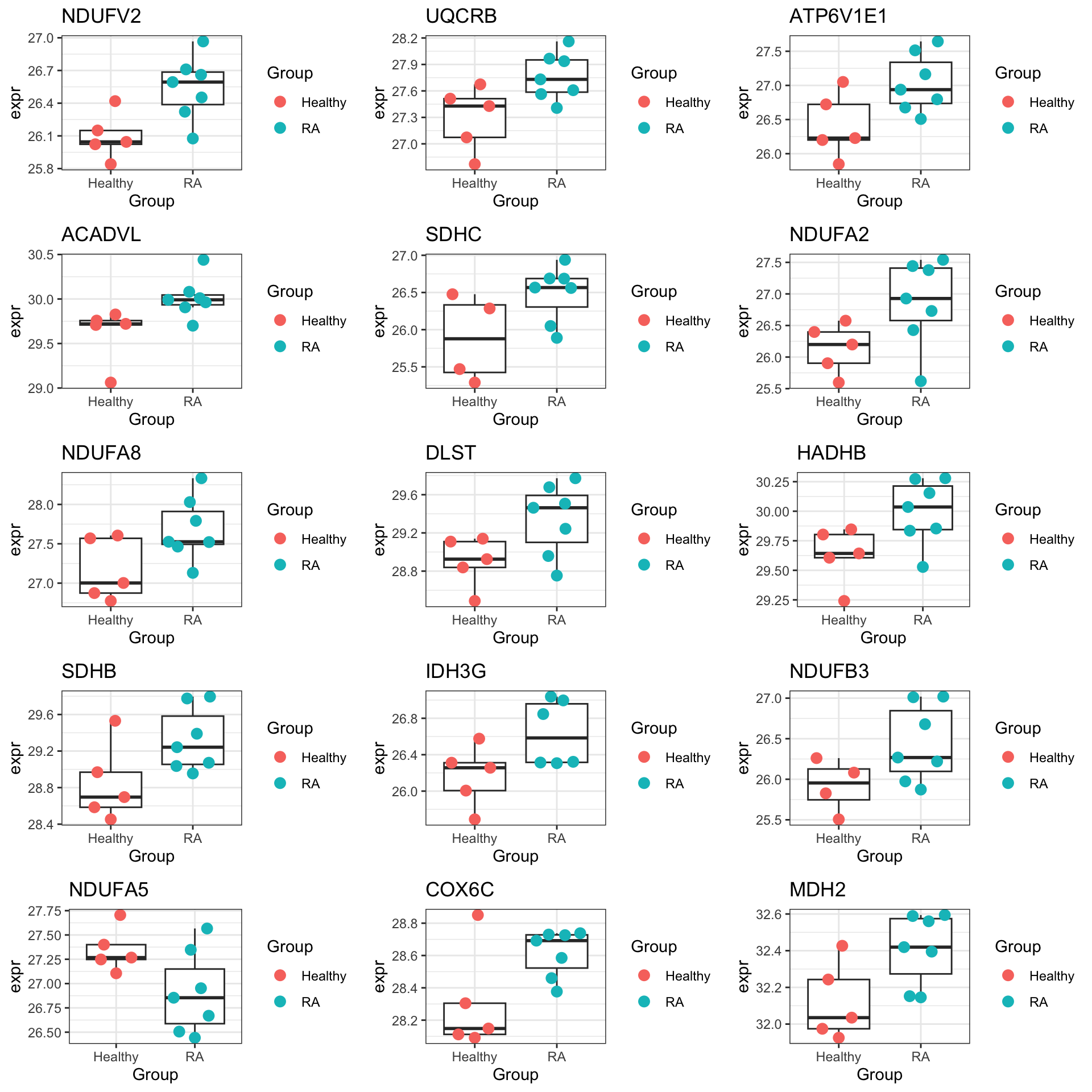

DNMT1 expression

countMat <- assays(protSub)[["imputed"]]
resDNMT1 <- filter(resTab, str_detect(symbol,"DNMT1"))
plotTab <- tibble(expr = countMat[resDNMT1$name,],
                Group = protSub$Group) 
ggplot(plotTab, aes(x=Group, y=expr)) +
    geom_boxplot(outlier.shape = NA) +
    ggbeeswarm::geom_quasirandom(aes(color = Group), size=3) +
    ggtitle("DNMT1") +
    theme_bw()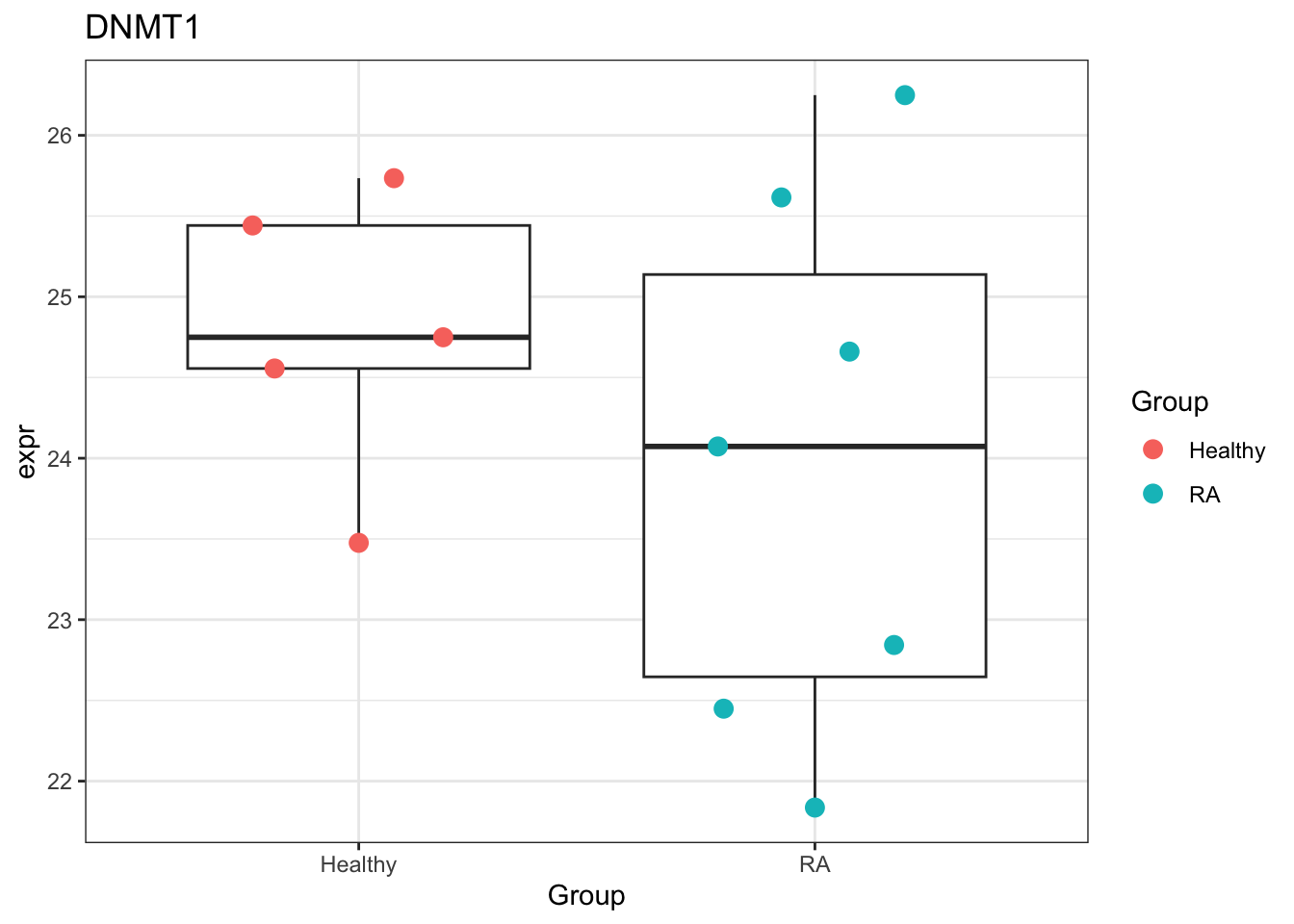

Power analysis to estimate sample size

rowData(protSub)$imputed <- NULL
protTab <- jyluMisc::sumToTidy(protSub)

meanTab <- protTab %>%
    group_by(Group, ID) %>%
    summarise(mean = mean(imputed)) %>%
    pivot_wider(names_from = Group, values_from = mean)

sdTab <- protTab %>%
    group_by(ID) %>%
    summarise(sd = sd(imputed))

dTab <- left_join(meanTab, sdTab) %>%
    mutate(d= abs(RA-Healthy)/sd)

nTab <- lapply(seq(nrow(dTab)), function(i) {
    rec <- dTab[i,]
    n1 <- pwr.t.test(d = rec$d , sig.level = 0.05, 
                    power = 0.9, alternative = "two.sided")$n
    n2 <- pwr.t.test(d = rec$d , sig.level = 0.01, 
                    power = 0.9, alternative = "two.sided")$n
    tibble(ID = rec$ID, 
           n0.05 = as.integer(n1), n0.01=as.integer(n2))
}) %>% bind_rows() %>% 
    arrange(n0.05) %>%
    mutate(name = rowData(protSub[ID,])$name)

Sample size table

nTab %>% select(-ID) %>% 
    DT::datatable()

Sample size versus DE proteins detectable.

plotTab <- lapply(seq(0.01, 1.5, length.out=100), function(x) {
     tibble(nCall = nrow(filter(dTab, d > x)),
            nSample = pwr.t.test(d = x , sig.level = 0.05, 
                                 power = 0.8, type = "two.sample")$n)
}) %>% bind_rows() %>%
    arrange(nCall) %>% filter(nCall >0)

ggplot(plotTab, aes(x=nCall, y=nSample)) +
    geom_line() + geom_point() +
    ylim(0,100) + xlim(0,1500) +
    ylab("sample per group") +
    xlab("differentially expressed proteins at P=0.05") +
    theme_bw()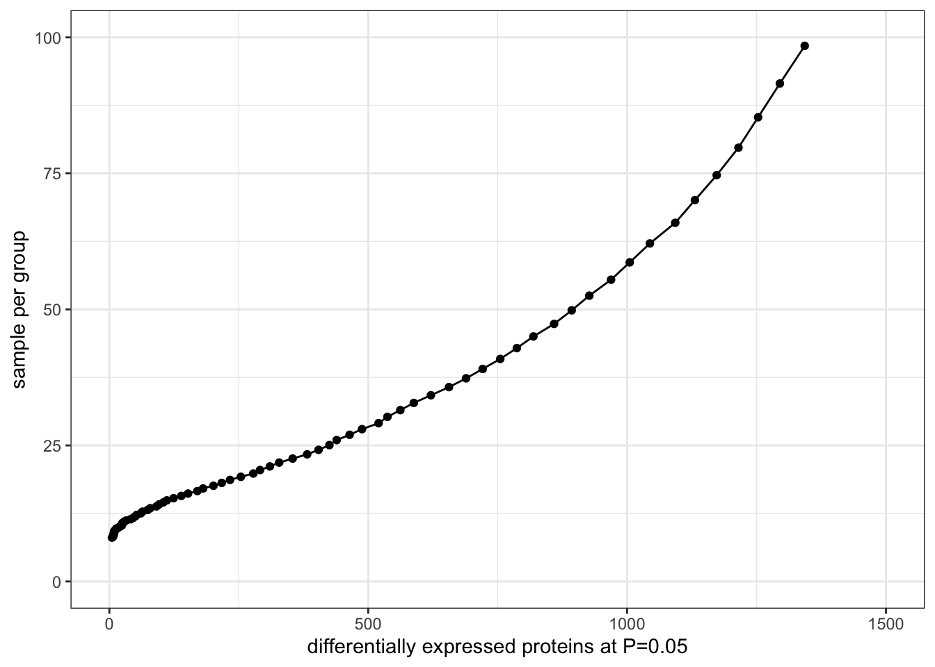 

(n = sample in each group)

Session information

sessionInfo()

R version 4.2.0 (2022-04-22)
Platform: x86_64-apple-darwin17.0 (64-bit)
Running under: macOS Big Sur/Monterey 10.16

Matrix products: default
BLAS:   /Library/Frameworks/R.framework/Versions/4.2/Resources/lib/libRblas.0.dylib
LAPACK: /Library/Frameworks/R.framework/Versions/4.2/Resources/lib/libRlapack.dylib

locale:
[1] en_US.UTF-8/en_US.UTF-8/en_US.UTF-8/C/en_US.UTF-8/en_US.UTF-8

attached base packages:
[1] stats4    stats     graphics  grDevices utils     datasets  methods  
[8] base     

other attached packages:
 [1] piano_2.12.0                proDA_1.10.0               
 [3] pheatmap_1.0.12             limma_3.52.2               
 [5] forcats_0.5.1               stringr_1.4.1              
 [7] dplyr_1.0.9                 purrr_0.3.4                
 [9] readr_2.1.2                 tidyr_1.2.0                
[11] tibble_3.1.8                ggplot2_3.4.1              
[13] tidyverse_1.3.2             SummarizedExperiment_1.26.1
[15] GenomicRanges_1.48.0        GenomeInfoDb_1.32.2        
[17] IRanges_2.30.0              S4Vectors_0.34.0           
[19] MatrixGenerics_1.8.1        matrixStats_0.62.0         
[21] jyluMisc_0.1.5              pwr_1.3-0                  
[23] vsn_3.64.0                  Biobase_2.56.0             
[25] BiocGenerics_0.42.0        

loaded via a namespace (and not attached):
  [1] DEP_1.18.0             utf8_1.2.2             shinydashboard_0.7.2  
  [4] gmm_1.6-6              tidyselect_1.1.2       htmlwidgets_1.5.4     
  [7] grid_4.2.0             BiocParallel_1.30.3    norm_1.0-10.0         
 [10] maxstat_0.7-25         munsell_0.5.0          codetools_0.2-18      
 [13] preprocessCore_1.58.0  DT_0.23                withr_2.5.0           
 [16] colorspace_2.0-3       highr_0.9              knitr_1.39            
 [19] rstudioapi_0.13        ggsignif_0.6.3         mzID_1.34.0           
 [22] labeling_0.4.2         git2r_0.30.1           slam_0.1-50           
 [25] GenomeInfoDbData_1.2.8 KMsurv_0.1-5           farver_2.1.1          
 [28] rprojroot_2.0.3        vctrs_0.5.2            generics_0.1.3        
 [31] TH.data_1.1-1          xfun_0.31              sets_1.0-21           
 [34] R6_2.5.1               doParallel_1.0.17      ggbeeswarm_0.6.0      
 [37] clue_0.3-61            MsCoreUtils_1.8.0      bitops_1.0-7          
 [40] cachem_1.0.6           fgsea_1.22.0           DelayedArray_0.22.0   
 [43] assertthat_0.2.1       promises_1.2.0.1       scales_1.2.0          
 [46] multcomp_1.4-19        googlesheets4_1.0.0    beeswarm_0.4.0        
 [49] gtable_0.3.0           extraDistr_1.9.1       Cairo_1.6-0           
 [52] affy_1.74.0            sandwich_3.0-2         workflowr_1.7.0       
 [55] rlang_1.0.6            mzR_2.30.0             GlobalOptions_0.1.2   
 [58] splines_4.2.0          rstatix_0.7.0          impute_1.70.0         
 [61] gargle_1.2.0           broom_1.0.0            BiocManager_1.30.18   
 [64] yaml_2.3.5             abind_1.4-5            modelr_0.1.8          
 [67] crosstalk_1.2.0        backports_1.4.1        httpuv_1.6.6          
 [70] tools_4.2.0            relations_0.6-12       affyio_1.66.0         
 [73] ellipsis_0.3.2         gplots_3.1.3           jquerylib_0.1.4       
 [76] RColorBrewer_1.1-3     MSnbase_2.22.0         plyr_1.8.7            
 [79] Rcpp_1.0.9             visNetwork_2.1.0       zlibbioc_1.42.0       
 [82] RCurl_1.98-1.7         ggpubr_0.4.0           GetoptLong_1.0.5      
 [85] cowplot_1.1.1          zoo_1.8-10             ggrepel_0.9.1         
 [88] haven_2.5.0            cluster_2.1.3          exactRankTests_0.8-35 
 [91] fs_1.5.2               magrittr_2.0.3         magick_2.7.3          
 [94] data.table_1.14.2      circlize_0.4.15        reprex_2.0.1          
 [97] survminer_0.4.9        pcaMethods_1.88.0      googledrive_2.0.0     
[100] mvtnorm_1.1-3          ProtGenerics_1.28.0    hms_1.1.1             
[103] shinyjs_2.1.0          mime_0.12              evaluate_0.15         
[106] xtable_1.8-4           XML_3.99-0.10          readxl_1.4.0          
[109] gridExtra_2.3          shape_1.4.6            compiler_4.2.0        
[112] ncdf4_1.19             KernSmooth_2.23-20     crayon_1.5.2          
[115] htmltools_0.5.4        later_1.3.0            tzdb_0.3.0            
[118] lubridate_1.8.0        DBI_1.1.3              dbplyr_2.2.1          
[121] ComplexHeatmap_2.12.0  tmvtnorm_1.5           MASS_7.3-58           
[124] Matrix_1.4-1           car_3.1-0              cli_3.4.1             
[127] imputeLCMD_2.1         marray_1.74.0          parallel_4.2.0        
[130] igraph_1.3.4           pkgconfig_2.0.3        km.ci_0.5-6           
[133] MALDIquant_1.21        xml2_1.3.3             foreach_1.5.2         
[136] vipor_0.4.5            bslib_0.4.1            XVector_0.36.0        
[139] drc_3.0-1              rvest_1.0.2            digest_0.6.30         
[142] rmarkdown_2.14         cellranger_1.1.0       fastmatch_1.1-3       
[145] survMisc_0.5.6         shiny_1.7.4            gtools_3.9.3          
[148] rjson_0.2.21           lifecycle_1.0.3        jsonlite_1.8.3        
[151] carData_3.0-5          fansi_1.0.3            pillar_1.8.0          
[154] lattice_0.20-45        fastmap_1.1.0          httr_1.4.3            
[157] plotrix_3.8-2          survival_3.4-0         glue_1.6.2            
[160] png_0.1-7              iterators_1.0.14       stringi_1.7.8         
[163] sass_0.4.2             caTools_1.18.2