Last updated: 2024-04-08

Checks: 5 1

Knit directory: RA_Tcell_omics/analysis/

This reproducible R Markdown analysis was created with workflowr (version 1.7.0). The Checks tab describes the reproducibility checks that were applied when the results were created. The Past versions tab lists the development history.

Environment: empty

Great job! The global environment was empty. Objects defined in the global environment can affect the analysis in your R Markdown file in unknown ways. For reproduciblity it’s best to always run the code in an empty environment.

Seed: set.seed(20221110)

The command set.seed(20221110) was run prior to running the code in the R Markdown file. Setting a seed ensures that any results that rely on randomness, e.g. subsampling or permutations, are reproducible.

Session information: recorded

Great job! Recording the operating system, R version, and package versions is critical for reproducibility.

Cache: none

Nice! There were no cached chunks for this analysis, so you can be confident that you successfully produced the results during this run.

File paths: relative

Great job! Using relative paths to the files within your workflowr project makes it easier to run your code on other machines.

Repository version: no version control

Tracking code development and connecting the code version to the results is critical for reproducibility. To start using Git, open the Terminal and type git init in your project directory.

This project is not being versioned with Git. To obtain the full reproducibility benefits of using workflowr, please see ?wflow_start.

Load libraries

library(vsn)
library(jyluMisc)
library(SummarizedExperiment)
library(tidyverse)
knitr::opts_chunk$set(warning = FALSE, message = FALSE)

Load sample annotations

patTab1 <- readxl::read_xlsx("../data/Data_2023-02-16/MultiOmics Patien Data.xlsx", sheet = 1) %>%
    filter(!is.na(Pseudonyme)) %>%
    dplyr::rename(sampleID = Pseudonyme) %>%
    mutate(sampleID = str_remove_all(sampleID," ")) %>%
    mutate(group = "RA") %>%
    dplyr::rename(`Date of Birth` = `Date of Birtrh`)
patTab2 <- readxl::read_xlsx("../data/Data_2023-02-16/MultiOmics Patien Data.xlsx", sheet = 2) %>%
    filter(!is.na(Pseudonyme)) %>%
    dplyr::rename(sampleID = Pseudonyme, `Date of sample` = `Date of Sample`) %>%
    mutate(sampleID = str_remove_all(sampleID," ")) %>%
    mutate(group = "HC") %>%
    mutate(`Date of Birth` = as.Date(as.character(`Date of Birth`), format = "%Y"))
patTab <- bind_rows(patTab1, patTab2) %>%
    distinct(sampleID, .keep_all = TRUE)

Choose useful data

patTab <- mutate(patTab, Age = as.numeric((`Date of sample` - `Date of Birth`)/365),
                 dateMeta = as.character(Metabolites),
                 dateProt = as.character(Proteome),
                 datePhos = as.character(Phosphoproteome),
                 dateMeth = as.character(Methylation),
                 dateFACS = as.character(Flowcytometry)) %>%
    dplyr::rename(BMI = `BMI(kg/(m^2))`, CRP = `CRP [mg/l]`) %>%
    mutate(CRP = as.numeric(str_remove_all(CRP, "<"))) %>%
    select(sampleID, Gender, Age, CCP, RF, GC, MTX, Leflunomid, Sulfasalazin, Quensyl, BMI, CRP,DAS28, group,
           dateMeta, dateProt, datePhos, dateMeth, dateFACS)

Sample metadata table

patTab %>% mutate_if(is.numeric, formatC, digits=1) %>% DT::datatable()

Process the the new metabolic table

metaTab1 <- readxl::read_xlsx("../data/Data_2023-02-16/Metabolites/20211022_results_GCMS_metabolomics_CD8_RAHC.xlsx", sheet = 1, skip = 1) %>%
    dplyr::rename(sampleID = `...1`) %>%
    pivot_longer(-sampleID, names_to = "feature", values_to = "count") %>%
    mutate(sheet = "Metabolites")
metaTab2 <- readxl::read_xlsx("../data/Data_2023-02-16/Metabolites/20211022_results_GCMS_metabolomics_CD8_RAHC.xlsx", sheet = 2, skip = 1) %>%
    dplyr::rename(sampleID = ProbenID) %>%
    pivot_longer(-sampleID, names_to = "feature", values_to = "count") %>%
    mutate(sheet = "AA-AC")

metaTab  <- bind_rows(metaTab1, metaTab2) %>%
    filter(!is.na(sampleID)) %>%
    left_join(patTab, by = "sampleID") %>%
    mutate(metabolite = feature)

seMeta <- jyluMisc::tidyToSum(metaTab, rowID = "feature", colID = "sampleID", values = "count", annoRow = c("sheet","metabolite"), 
                              annoCol = colnames(patTab)[2:ncol(patTab)])
dim(seMeta)

[1] 65 36

Why there are two sheets in the excel table, are there any difference in the measurement process? What is the difference between this data and previous data? Seems just more samples, the values are the same. Are they from different batches?

QC

plotTab <- metaTab 
metaMat <- assay(seMeta )

Feature distribution

Per-sample

Raw scale

ggplot(plotTab, aes(x=sampleID, y=count, fill = group)) +
    geom_boxplot() + geom_point() +
    theme(axis.text.x = element_text(angle = 90, hjust=1, vjust =0.5))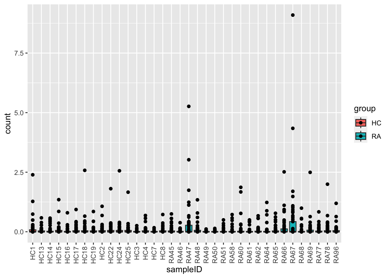

glog transformed

ggplot(plotTab, aes(x=sampleID, y=glog(count), fill = group)) +
    geom_boxplot() + geom_point() +
    theme(axis.text.x = element_text(angle = 90, hjust=1, vjust =0.5))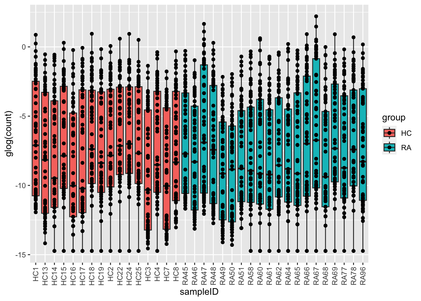

Per feature

Raw scale

ggplot(plotTab, aes(x=feature, y=count)) +
    geom_boxplot() + geom_point(aes(col=group)) +
    theme(axis.text.x = element_text(angle = 90, hjust=1, vjust =0.5))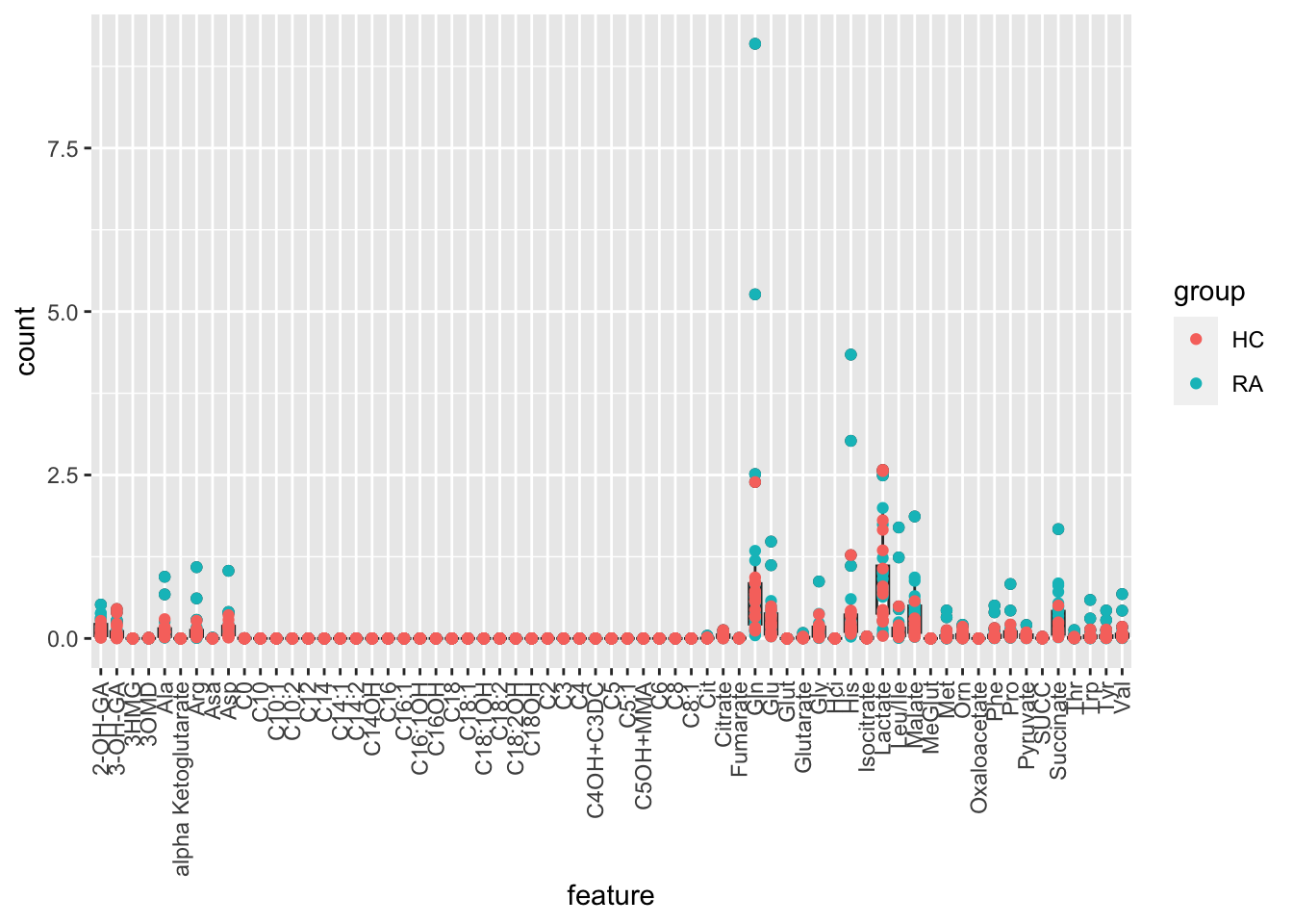

glog transformed

ggplot(plotTab, aes(x=feature, y=glog(count))) +
    geom_boxplot() + geom_point(aes(col= group)) +
    theme(axis.text.x = element_text(angle = 90, hjust=1, vjust =0.5))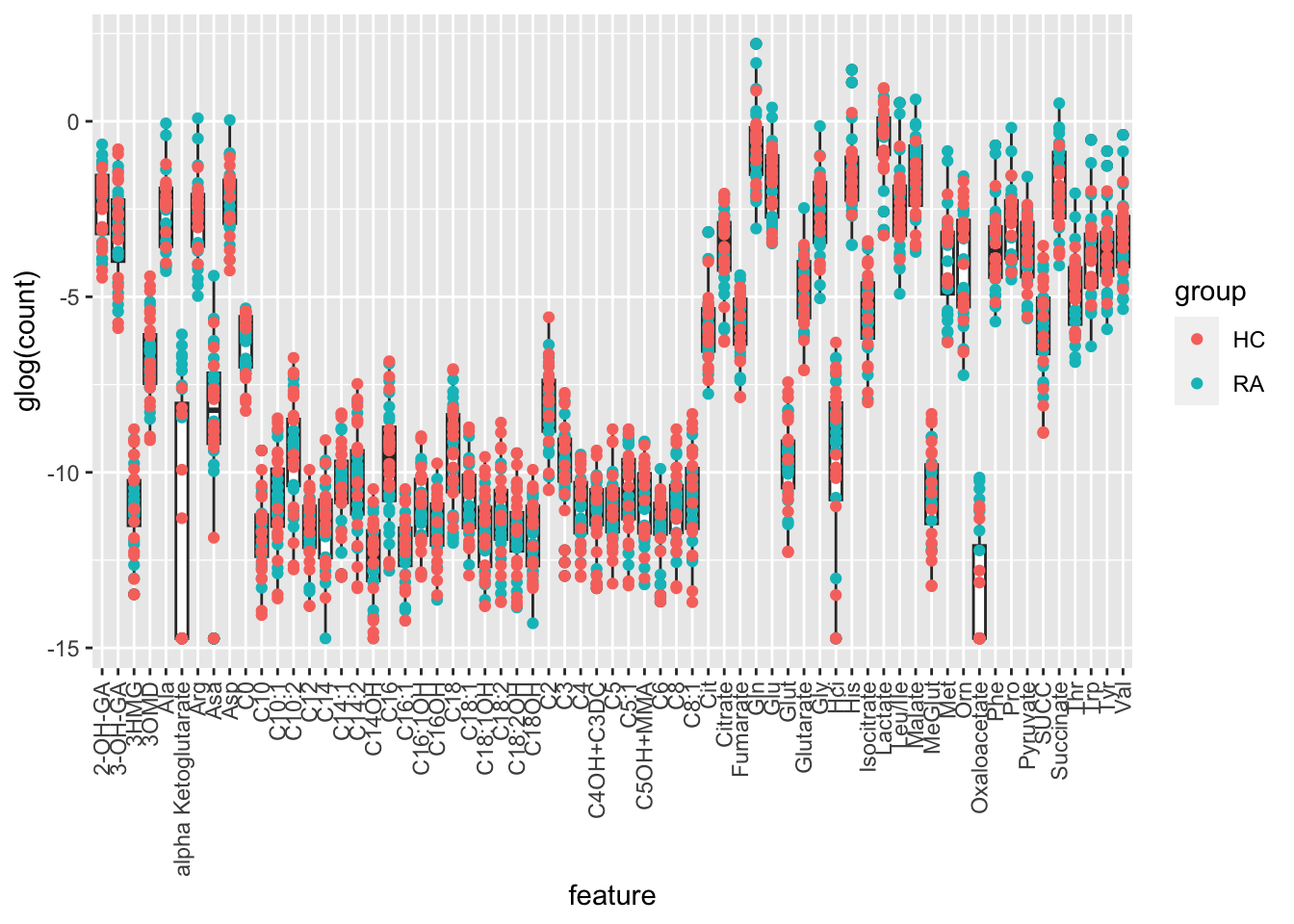

PCA

Raw scale

metaMat <- metaMat[,complete.cases(t(metaMat))]
pcRes <- prcomp(t(metaMat), scale. = FALSE, center = TRUE)
plotTab <- pcRes$x %>% as_tibble(rownames = "sampleID") %>%
    left_join(patTab, by = "sampleID")
ggplot(plotTab, aes(x=PC1, y=PC2, col = group, label = sampleID)) +
    geom_point() +
    geom_text()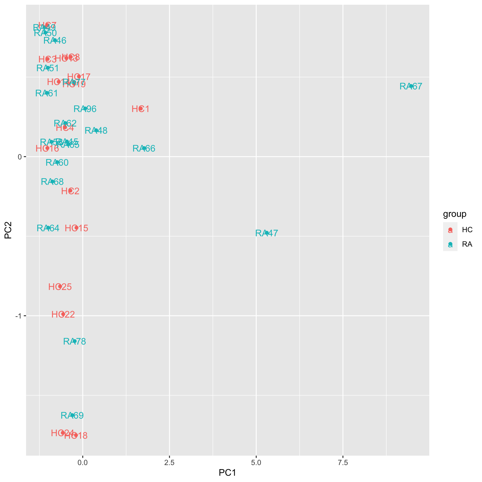

glog transformed

Colored by phenotype

metaMat <- jyluMisc::glog(metaMat)
pcRes <- prcomp(t(metaMat), scale. = FALSE, center = TRUE)
plotTab <- pcRes$x %>% as_tibble(rownames = "sampleID") %>%
    left_join(patTab, by = "sampleID")
ggplot(plotTab, aes(x=PC1, y=PC2, col = group, label = sampleID)) +
    geom_point() +
    geom_text()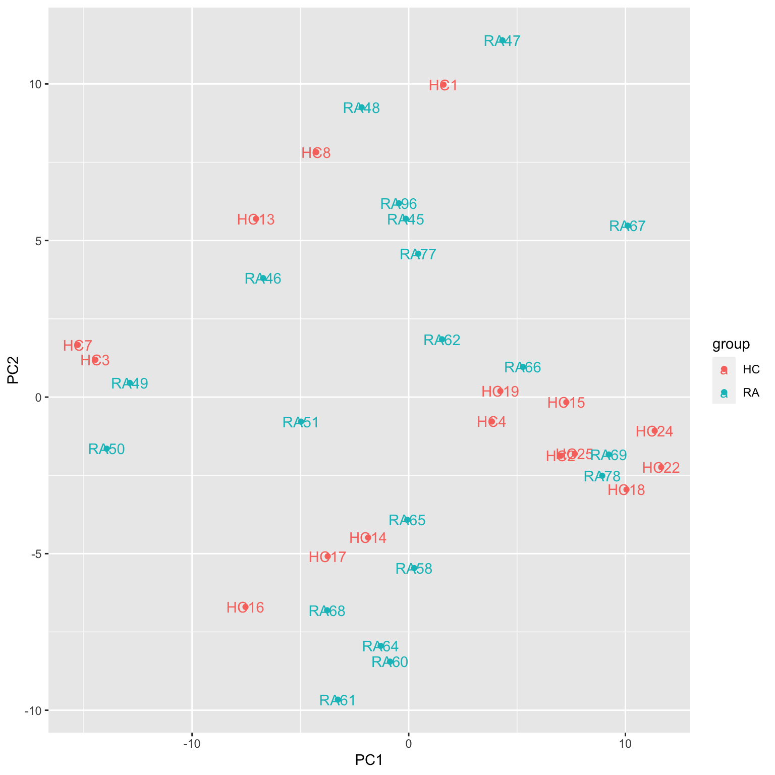

Colored by date of metabolic measurement

metaMat <- jyluMisc::glog(metaMat)
pcRes <- prcomp(t(metaMat), scale. = FALSE, center = TRUE)
plotTab <- pcRes$x %>% as_tibble(rownames = "sampleID") %>%
    left_join(patTab, by = "sampleID")
ggplot(plotTab, aes(x=PC1, y=PC2, col = dateMeta, label = sampleID)) +
    geom_point() +
    geom_text()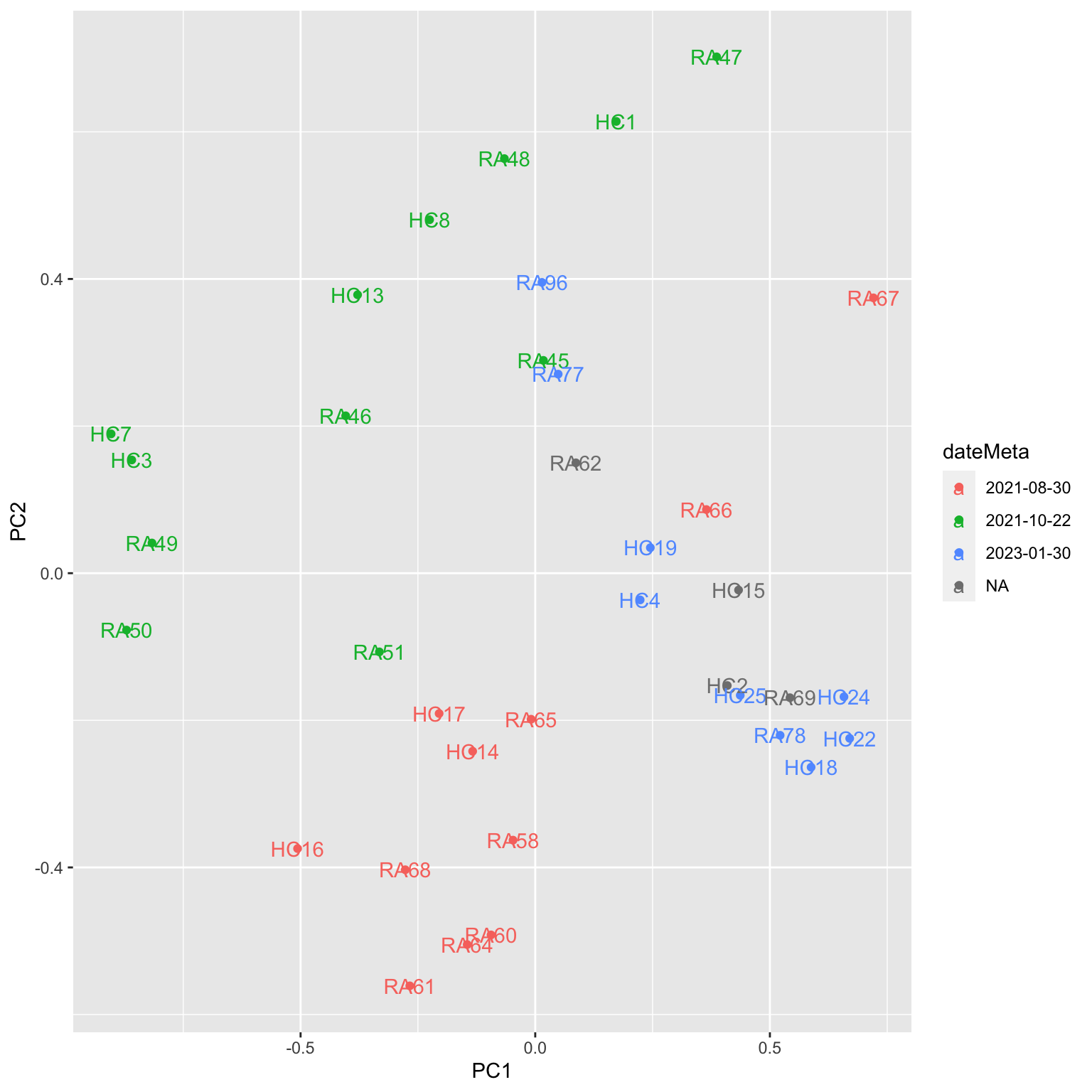

Batch effect could be observed
Two samples don’t have date information

Process Proteomics data

Map the sample name

sampleMap <- readxl::read_xlsx("../data/Data_2023-02-16/Proteome_Phosphome/sample submission naming.xlsx", col_names = c("id","sampleID")) %>%
    mutate(id = sprintf("%s%02d","Sample",id))

Read in additional proteomic sample metadata

smpMeta <- readxl::read_xlsx("../data/TF0489/Sample-Information.xlsx") %>%
    filter(!is.na(`Patient Group`))
smpMeta <- smpMeta[,c(1,5,6,7,8)]
colnames(smpMeta) <- c("sampleID","protConc","quantStart","sampleVol","bufferComp")
smpMeta <- mutate(smpMeta, sampleID = paste0("Sample",sprintf("%02s",sampleID)))

It seems compared to previous proteomic data, in this data, the replicates are removed and buffer A was prioritized.

Read data table

protTab <- readxl::read_xlsx("../data/Data_2023-02-16/Proteome_Phosphome/TF0489-3_results/TF0489-3_filtered_proteinGroups.xlsx") %>%
    filter(!`Potential contaminant` %in% "+") %>%
    select(`Majority protein IDs`, `Gene names`, contains("LFQ intensity")) %>%
    dplyr::rename(name = "Majority protein IDs", symbol = "Gene names") %>%
    pivot_longer(-c(name, symbol), names_to = "sampleID", values_to = "count") %>%
    mutate(sampleID = str_remove(sampleID, "LFQ intensity ")) %>%
    filter(count>0) %>% left_join(smpMeta, by = "sampleID") %>%
    mutate(sampleID = sampleMap[match(sampleID,sampleMap$id),]$sampleID) %>%
    left_join(patTab, by = "sampleID")
idMap <- unique(protTab$name)
idMap <- structure(paste0("prot",seq_along(idMap)), names = idMap)
protTab <- mutate(protTab, ID = idMap[name])

Choose the first symbol if multiple symbols are present in the symbol column

# Get the last symbol of a protein that has multiple gene symbols
getOneSymbol <- function(Gene) {
    outStr <- sapply(Gene, function(x) {
        sp <- str_split(x, ";")[[1]]
        sp[length(sp)]
    })
    names(outStr) <- NULL
    outStr
}
protTab$symbol <- getOneSymbol(protTab$symbol)

#only keep proteins with symbols
protTab <- filter(protTab, !symbol %in% c("",NA))

Created summarised experiment

seProt <- jyluMisc::tidyToSum(protTab, "ID", "sampleID","count",
                               annoRow = c("ID","name","symbol"),
                               annoCol = c(colnames(patTab),"protConc", "quantStart", "sampleVol", "bufferComp"))

QA

Data completeness per sample

countMat <- assay(seProt)
plotTab <- tibble(sample = colnames(seProt), 
                  perNA = colSums(is.na(countMat))/nrow(countMat))
ggplot(plotTab, aes(x=sample, y=1-perNA)) +
    geom_bar(stat = "identity") +
    ylab("completeness") +
    theme(axis.text.x = element_text(angle = 90, hjust = 1, vjust=0))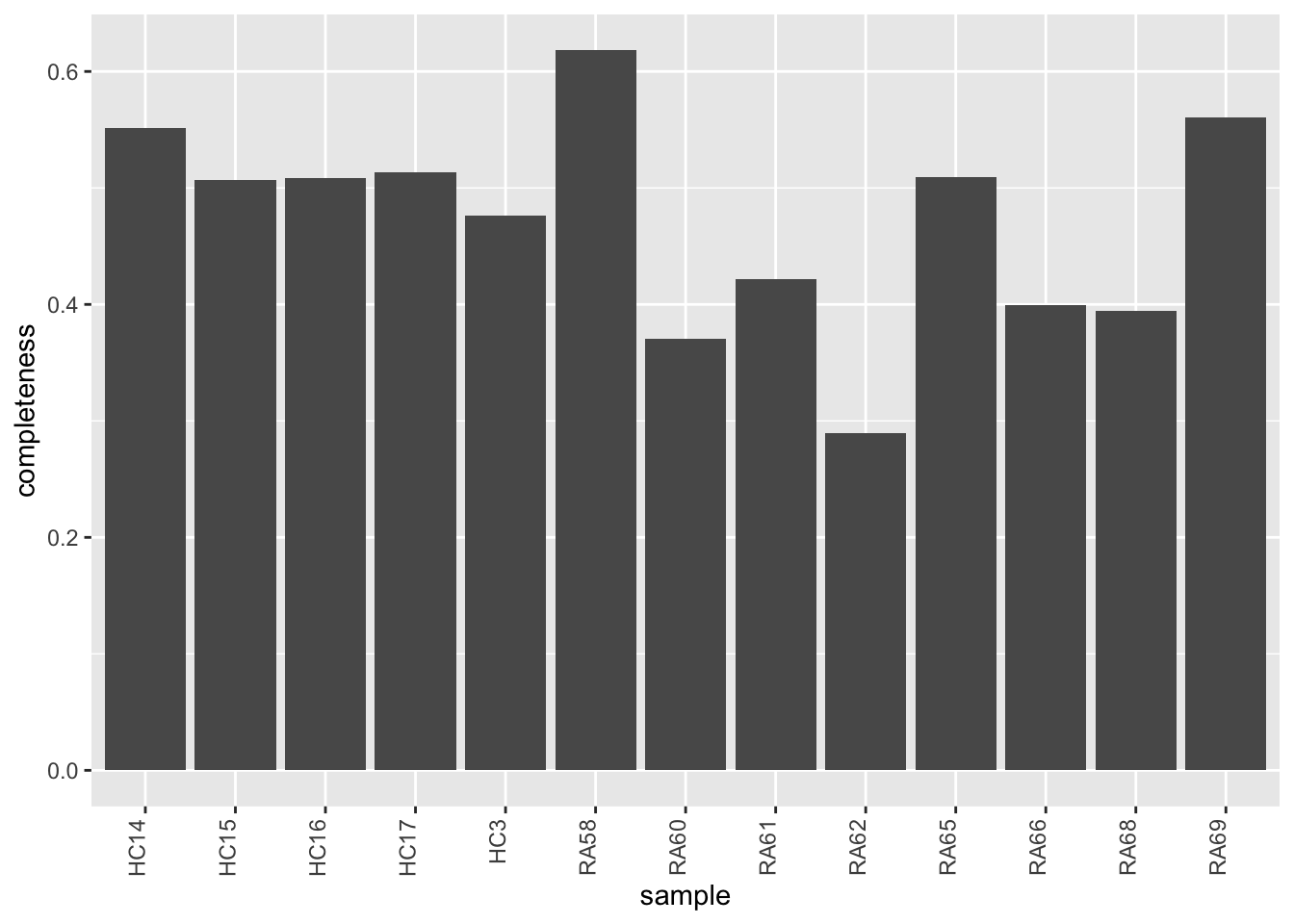

Plot a cumulative curve of missing value cut-off and remaining number of features

missRate <- tibble(id = rownames(countMat),
                   rate = rowSums(is.na(countMat))/ncol(countMat))
cumTab <- lapply(seq(0,1,0.05), function(cutRate) {
    tibble(cut= cutRate,
           per = sum(missRate$rate <= cutRate)/nrow(missRate))
} ) %>%
    bind_rows()
ggplot(cumTab, aes(x=cut,y=per)) +
    geom_line() +
    xlab("Allowed missing value rate") +
    ylab("Percentage of remaining features")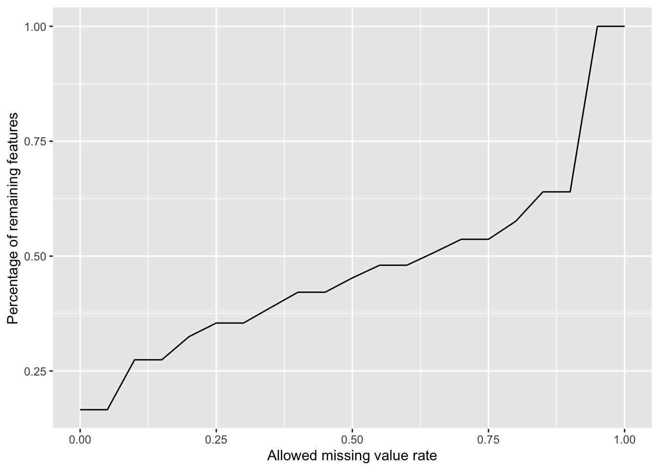

Missing value heatmap to check missing value structure

Visualize the missing value pattern

DEP::plot_missval(seProt)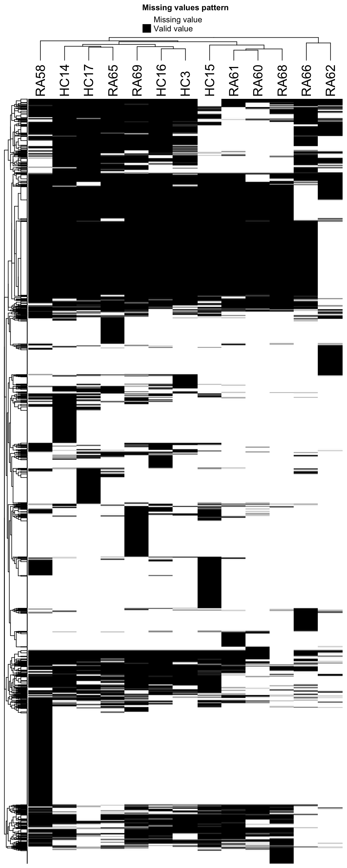

Looks pretty sparse, maybe due to the DDA data aquisition method

Keep proteins detected in at least half of the sample (missing rate <= 0.5)

protFilt <- seProt[filter(missRate, rate <=0.5)$id,]
dim(protFilt)

[1] 2342   13

Data distribution

countMat <- assay(protFilt)
countTab <- countMat %>% as_tibble(rownames = "id") %>% 
    pivot_longer(-id) %>%
    filter(!is.na(value)) %>%
    mutate(log2Val = log2(value))

ggplot(countTab, aes(x=name, y=log2Val)) +
    geom_boxplot() + geom_point()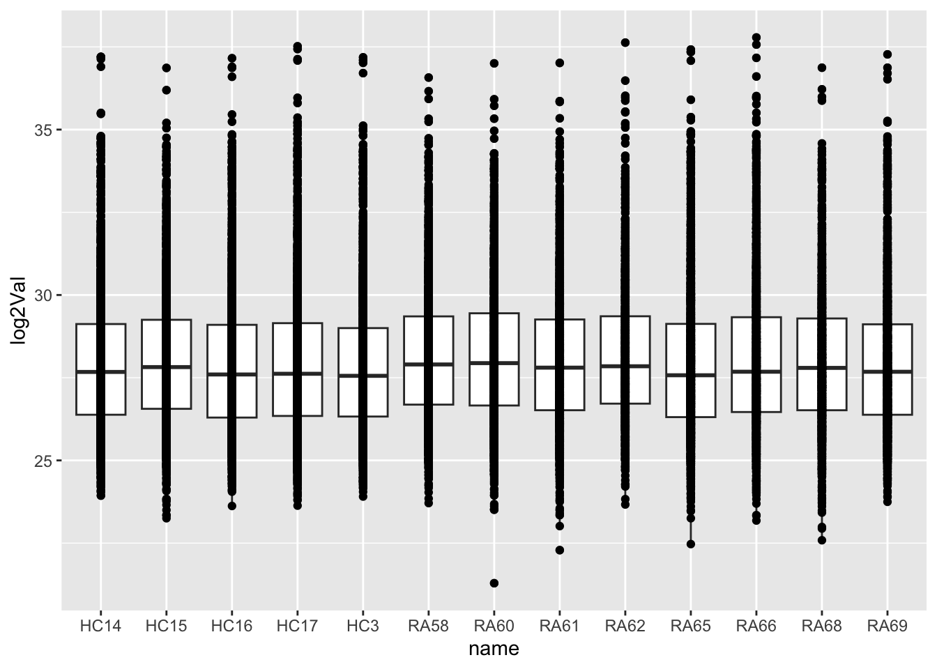

Imputation and normalization

Vst

protMat <- assay(protFilt)
fitVsn <- vsn::vsnMatrix(protMat)
normMat <- vsn::predict(fitVsn, newdata = protMat)
protNorm <- protFilt
assay(protNorm) <- normMat

Imputation

protImp <- DEP::impute(protNorm, "QRILC")
assays(protFilt)[["norm"]] <- normMat
assays(protFilt)[["imputed"]] <- assay(protImp)
rowData(protFilt) <- rowData(protImp)

Distribution after normalizaiton

countMat <- assays(protFilt)[["imputed"]]
countTab <- countMat %>% as_tibble(rownames = "id") %>% 
    pivot_longer(-id) %>%
    filter(!is.na(value))
ggplot(countTab, aes(x=name, y=value)) +
    geom_boxplot() + geom_point()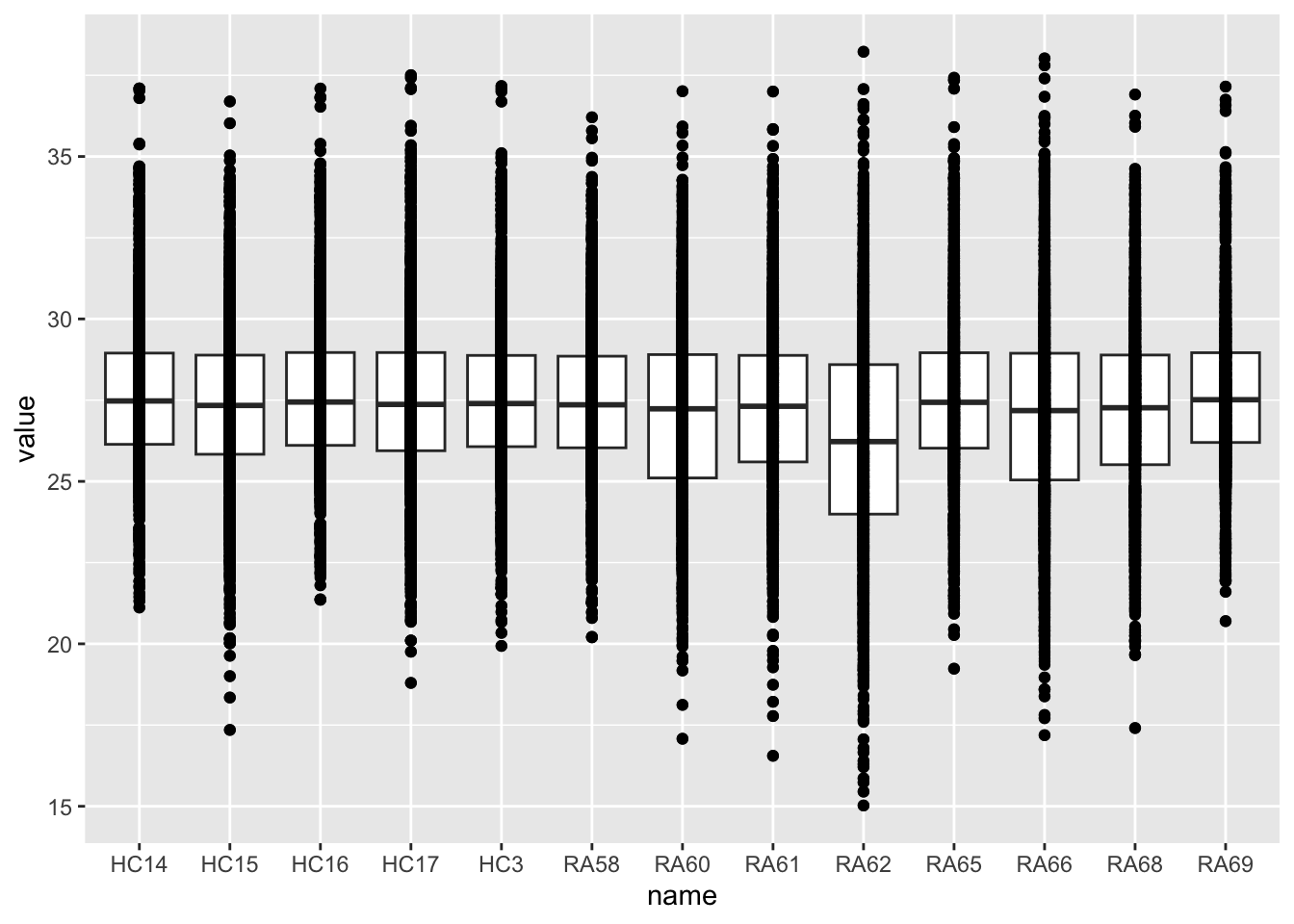

Mean versus variant plot

plotTab <- tibble(meanVal = rowMeans(countMat),
                  var = apply(countMat, 1, var))
ggplot(plotTab, aes(x=meanVal,y=var)) +
    geom_point()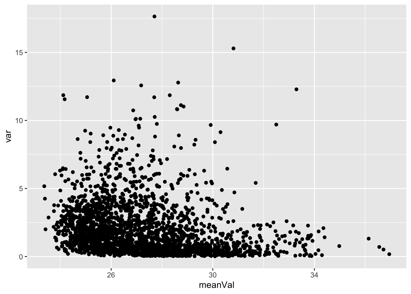

Heatmap visualization

library(pheatmap)
#select top 1000 most variant
colAnno <- colData(protFilt) %>% data.frame()
colAnno <- colAnno[,c("Gender","group","dateProt","protConc","quantStart","sampleVol","bufferComp")]
#colAnno[["sampleName"]] <- NULL
plotMat <- countMat[order(plotTab$var, decreasing = TRUE)[1:1000],]
pheatmap(plotMat, show_rownames = FALSE, scale = "row", 
         annotation_col = colAnno,
         clustering_method = "ward.D2")

Buffer composition and startQuant could be potential counfunding factor

PCA

prRes <- prcomp(t(plotMat), scale. = FALSE, center = TRUE)
plotTab <- prRes$x %>% as_tibble(rownames = "sampleID") %>%
    left_join(as_tibble(colAnno, rownames = "sampleID"))
ggplot(plotTab, aes(x=PC1, y=PC2, col = group)) +
    geom_point() +
    ggrepel::geom_text_repel(aes(label = sampleID))

RA62 looks like an outlier

Remove one potential outlier, RA62 and redo the preprocessing

Subset

protSub <- seProt[,seProt$sampleID != "RA62"]

#remove proteins with more than 50% missing values
protSub <- protSub[rowSums(is.na(assay(protSub)))/ncol(protSub)<=0.5,]

Vst

protMat <- assay(protSub)
fitVsn <- vsn::vsnMatrix(protMat)
normMat <- vsn::predict(fitVsn, newdata = protMat)
protNorm <- protSub
assay(protNorm) <- normMat

Imputation

protImp <- DEP::impute(protNorm, "QRILC")
assays(protSub)[["norm"]] <- normMat
assays(protSub)[["imputed"]] <- assay(protImp)

Redo pca

Color by group

plotMat <- assays(protSub)[["imputed"]]
prRes <- prcomp(t(plotMat), scale. = TRUE, center = TRUE)
plotTab <- prRes$x %>% as_tibble(rownames = "sampleID") %>%
    left_join(as_tibble(colAnno, rownames = "sampleID"))
ggplot(plotTab, aes(x=PC1, y=PC2, col = group)) +
    geom_point() +
    ggrepel::geom_text_repel(aes(label = sampleID))

Looks better.

Color by buffer composition

plotMat <- assays(protSub)[["imputed"]]
prRes <- prcomp(t(plotMat), scale. = TRUE, center = TRUE)
plotTab <- prRes$x %>% as_tibble(rownames = "sampleID") %>%
    left_join(as_tibble(colAnno, rownames = "sampleID"))
ggplot(plotTab, aes(x=PC1, y=PC2, col = bufferComp)) +
    geom_point() +
    ggrepel::geom_text_repel(aes(label = sampleID))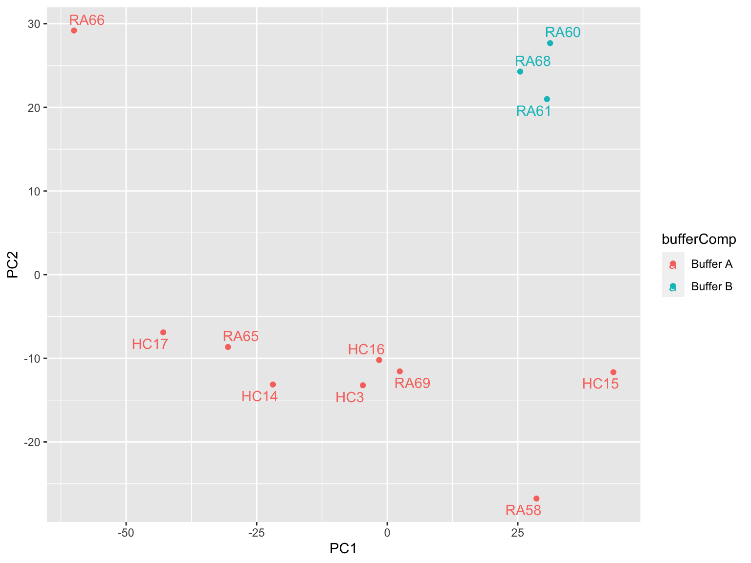

Phospho-proteomics

Read data table

phosTab <- readxl::read_xlsx("../data/Data_2023-02-16/Proteome_Phosphome/TF0489-3_results/TF0489-3_filtered_PhosphoSTY.xlsx") %>%
    filter(!`Potential contaminant` %in% "+") %>% 
    select(Proteins, `Leading proteins`, Position, `Gene names`, `Amino acid`,
           matches("(Intensity|Score|Score diff|Localization prob) Sample..$")) %>%
    pivot_longer(matches("Sample..$")) %>%
    mutate(sampleID = str_extract(name, "Sample.."),
           type = str_remove(name," Sample..")) %>%
    select(-name) %>%
    pivot_wider(names_from = type, values_from = value) %>%
    filter(`Localization prob` >= 0.75,
           `Score diff` >= 5,
           Score >= 10, 
           Intensity >0) %>%
    select(-c(`Localization prob`, `Score diff`, Score)) %>%
    left_join(smpMeta, by = "sampleID") %>%
    mutate(sampleID = sampleMap[match(sampleID,sampleMap$id),]$sampleID) %>%
    dplyr::rename(name = "Leading proteins", symbol = "Gene names", AA = "Amino acid", count = "Intensity") %>%
    mutate(symbol = getOneSymbol(symbol)) %>%
    mutate(siteID = paste0(Proteins,"_",Position),
           site = paste0(symbol,"_",AA,Position)) %>%
    filter(!symbol %in% c(NA,""))

idMap <- unique(phosTab$siteID)
idMap <- structure(paste0("phos",seq_along(idMap)), names = idMap)

phosTab <- mutate(phosTab, ID = idMap[siteID]) %>%
    left_join(patTab, by = "sampleID")

Created summarised experiment

sePhos <- jyluMisc::tidyToSum(phosTab, "ID", "sampleID","count",
                               annoRow = c("ID","name","symbol", "site","siteID", "Position", "AA"),
                               annoCol = c(colnames(patTab),"protConc", "quantStart", "sampleVol", "bufferComp"))

QA

Data completeness per sample

countMat <- assay(sePhos)
plotTab <- tibble(sample = colnames(sePhos), 
                  perNA = colSums(is.na(countMat))/nrow(countMat))
ggplot(plotTab, aes(x=sample, y=1-perNA)) +
    geom_bar(stat = "identity") +
    ylab("completeness") +
    theme(axis.text.x = element_text(angle = 90, hjust = 1, vjust=0))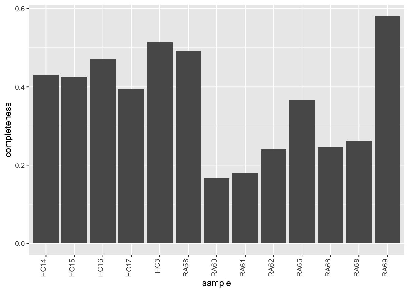

Plot a cumulative curve of missing value cut-off and remaining number of features

missRate <- tibble(id = rownames(countMat),
                   rate = rowSums(is.na(countMat))/ncol(countMat))
cumTab <- lapply(seq(0,1,0.05), function(cutRate) {
    tibble(cut= cutRate,
           per = sum(missRate$rate <= cutRate)/nrow(missRate))
} ) %>%
    bind_rows()
ggplot(cumTab, aes(x=cut,y=per)) +
    geom_line() +
    xlab("Allowed missing value rate") +
    ylab("Percentage of remaining features")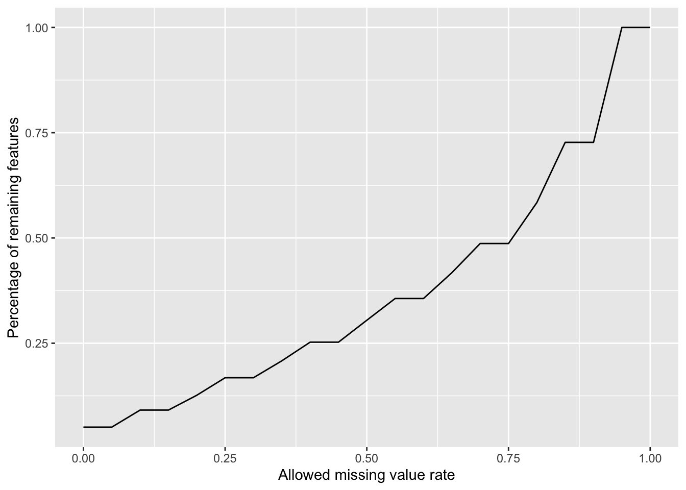

Missing value heatmap to check missing value structure

DEP::plot_missval(sePhos)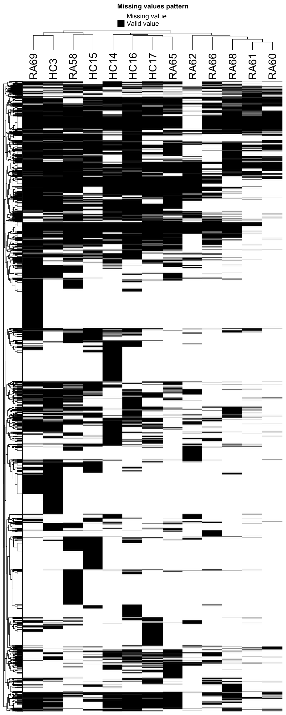

Also looks very sparse.

Keep proteins detected in at least half of the sample (missing rate <= 0.5)

phosFilt <- sePhos[filter(missRate, rate <=0.5)$id,]
dim(phosFilt)

[1] 2831   13

Data distribution

countMat <- assay(phosFilt)
countTab <- countMat %>% as_tibble(rownames = "id") %>% 
    pivot_longer(-id) %>%
    filter(!is.na(value)) %>%
    mutate(log2Val = log2(value))

ggplot(countTab, aes(x=name, y=log2Val)) +
    geom_boxplot() + geom_point()

Was phospho-enrichment performed? There’s strong difference in sample median RA60, 61, 68 are using different buffer and with different startQuant

Imputation and normalization

Vst

protMat <- assay(phosFilt)
fitVsn <- vsn::vsnMatrix(protMat)
normMat <- vsn::predict(fitVsn, newdata = protMat)
phosNorm <- phosFilt
assay(phosNorm) <- normMat

Imputation

protImp <- DEP::impute(phosNorm, "QRILC")
assays(phosFilt)[["norm"]] <- normMat
assays(phosFilt)[["imputed"]] <- assay(protImp)
rowData(phosFilt) <- rowData(protImp)

Distribution after normalizaiton

countMat <- assays(phosFilt)[["imputed"]]
countTab <- countMat %>% as_tibble(rownames = "id") %>% 
    pivot_longer(-id) %>%
    filter(!is.na(value))
ggplot(countTab, aes(x=name, y=value)) +
    geom_boxplot() + geom_point()

Mean versus variant plot

plotTab <- tibble(meanVal = rowMeans(countMat),
                  var = apply(countMat, 1, var))
ggplot(plotTab, aes(x=meanVal,y=var)) +
    geom_point()

Heatmap visualization

library(pheatmap)
#select top 1000 most variant
colAnno <- colData(phosFilt) %>% data.frame()
colAnno <- colAnno[,c("Gender","group", "datePhos", "protConc", "quantStart", "sampleVol", "bufferComp")]
#colAnno[["sampleName"]] <- NULL
plotMat <- countMat[order(plotTab$var, decreasing = TRUE)[1:1000],]
pheatmap(plotMat, show_rownames = FALSE, scale = "row", 
         annotation_col = colAnno,
         clustering_method = "ward.D2")

PCA

prRes <- prcomp(t(plotMat), scale. = TRUE, center = TRUE)
plotTab <- prRes$x %>% as_tibble(rownames = "sampleID") %>%
    left_join(as_tibble(colAnno, rownames = "sampleID"))
ggplot(plotTab, aes(x=PC1, y=PC2, col = group)) +
    geom_point() +
    ggrepel::geom_text_repel(aes(label = sampleID))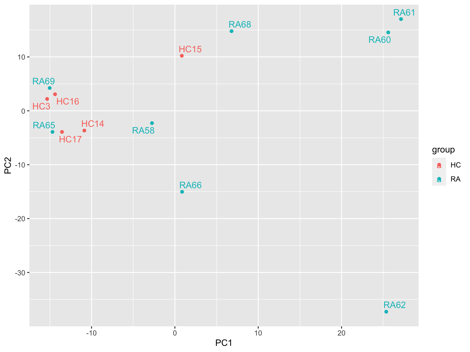

RA62 here may also be an outliers, although not as strong as proteomics Similar to the proteomics data, RA68,RA66,RA60 and RA61 are more separated to HC samples than other RA samples

Colored by buffer composition

prRes <- prcomp(t(plotMat), scale. = TRUE, center = TRUE)
plotTab <- prRes$x %>% as_tibble(rownames = "sampleID") %>%
    left_join(as_tibble(colAnno, rownames = "sampleID"))
ggplot(plotTab, aes(x=PC1, y=PC2, col = bufferComp)) +
    geom_point() +
    ggrepel::geom_text_repel(aes(label = sampleID))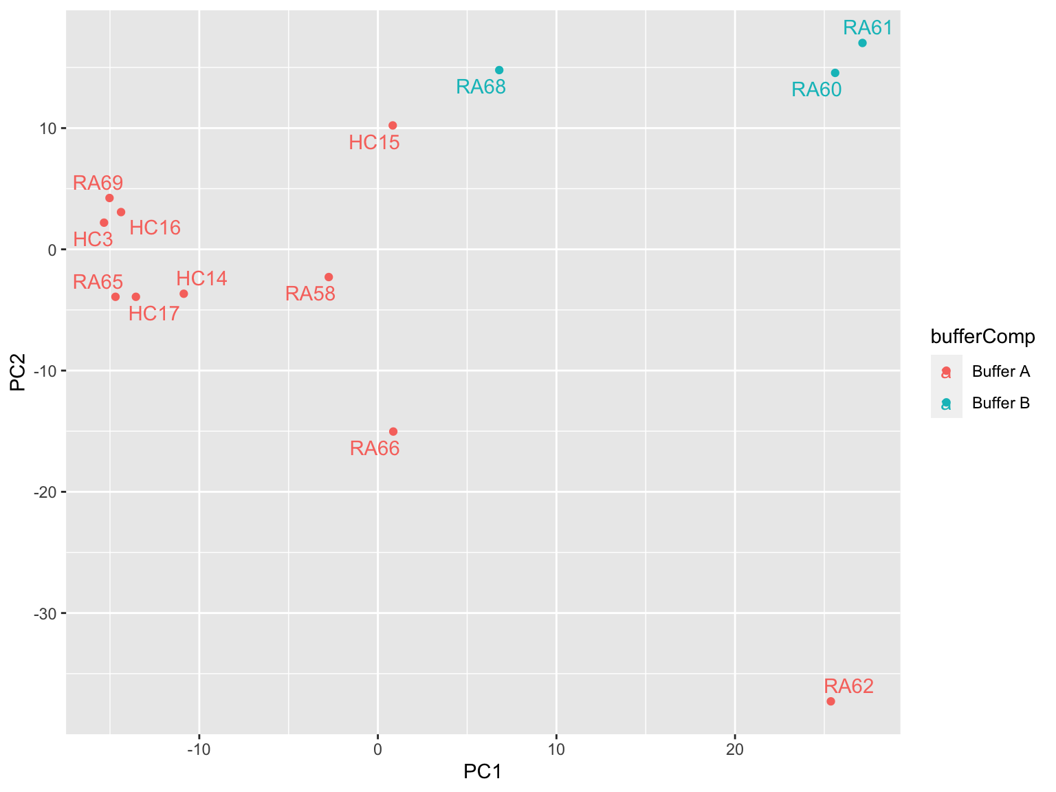

Remove one potential outlier, RA62 and redo preprocessing

phosSub <- phosFilt[,phosFilt$sampleID != "RA62"]

Subset

phosSub <- sePhos[,sePhos$sampleID != "RA62"]

#remove proteins with more than 50% missing values
phosSub <- phosSub[rowSums(is.na(assay(phosSub)))/ncol(phosSub)<=0.5,]

Vst

protMat <- assay(phosSub)
fitVsn <- vsn::vsnMatrix(protMat)
normMat <- vsn::predict(fitVsn, newdata = protMat)
phosNorm <- phosSub
assay(phosNorm) <- normMat

Imputation

protImp <- DEP::impute(phosNorm, "QRILC")
assays(phosSub)[["norm"]] <- normMat
assays(phosSub)[["imputed"]] <- assay(protImp)

Redo pca

plotMat <- assays(phosSub)[["imputed"]]
prRes <- prcomp(t(plotMat), scale. = TRUE, center = TRUE)
plotTab <- prRes$x %>% as_tibble(rownames = "sampleID") %>%
    left_join(as_tibble(colAnno, rownames = "sampleID"))
ggplot(plotTab, aes(x=PC1, y=PC2, col = group)) +
    geom_point() +
    ggrepel::geom_text_repel(aes(label = sampleID))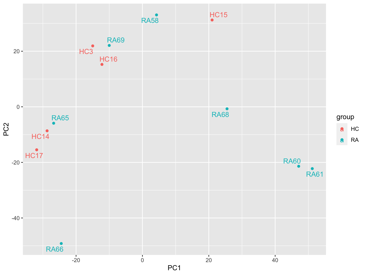

Colored by buffer composition

plotMat <- assays(phosSub)[["imputed"]]
prRes <- prcomp(t(plotMat), scale. = TRUE, center = TRUE)
plotTab <- prRes$x %>% as_tibble(rownames = "sampleID") %>%
    left_join(as_tibble(colAnno, rownames = "sampleID"))
ggplot(plotTab, aes(x=PC1, y=PC2, col = bufferComp)) +
    geom_point() +
    ggrepel::geom_text_repel(aes(label = sampleID))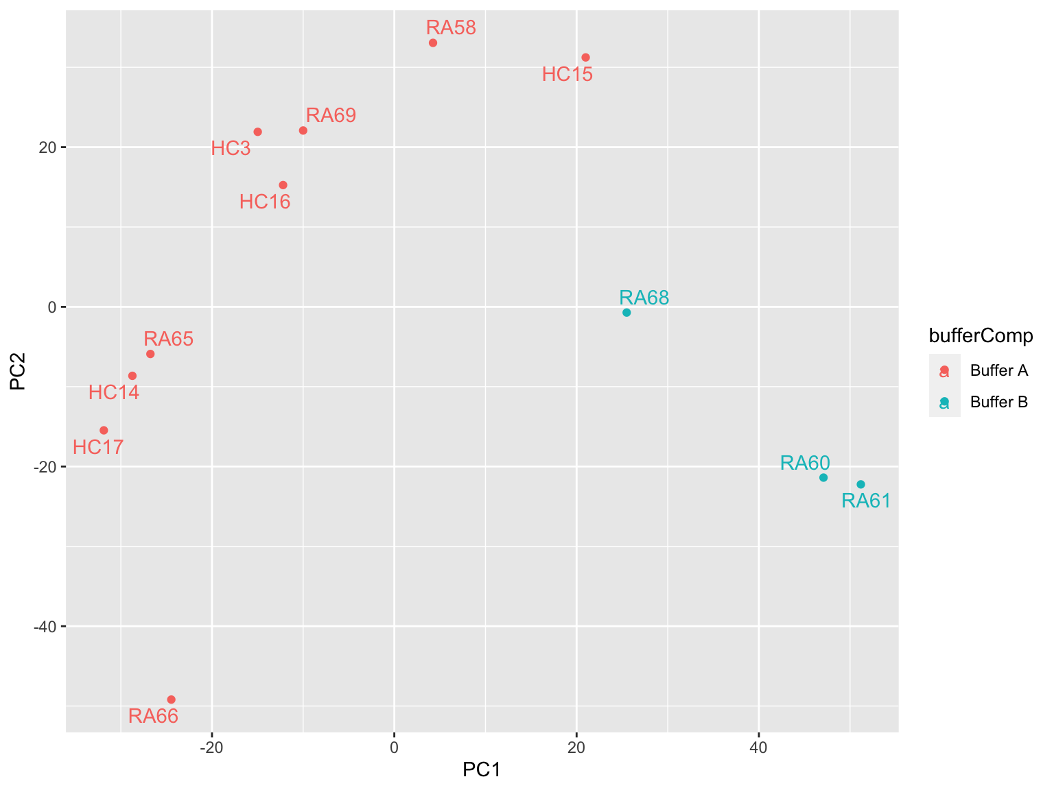

Phosphorylation normalized by protein expression

protBaseTab <- sumToTidy(protSub) %>%
    select(colID, norm, name) %>%
    group_by(colID, name) %>%
    summarise(protNorm = mean(norm, na.rm=TRUE))
phosRatioTab <- sumToTidy(phosSub) %>%
    select(rowID, colID, norm, name, site, symbol, bufferComp) %>%
    left_join(protBaseTab, by = c("colID","name")) %>%
    mutate(ratio = norm-protNorm) %>%
    filter(!is.na(ratio))
seRatio <- tidyToSum(phosRatioTab, "rowID","colID","ratio", c("name","site","symbol"), annoCol = c("colID","bufferComp"))

Methylation data

Use the processed methylation data from another script

load("../output/methData_20221118.RData")

Filtering, only keep the top 5000 most variant genes for the multi-omics analysis

#remove genes on X,Y chromosome
methData <- methData[!seqnames(methData) %in% c("chrX","chrY"),]
methMat <- assays(methData)[["M"]]

#keep 5000 most variable CpG
sds <- genefilter::rowSds(methMat)
methMat <- methMat[order(sds, decreasing = T)[1:5000],]
colnames(methMat) <- methData$Sample_Name

FACS data

facsTab <- readxl::read_xlsx("../data/Data_2023-02-16/FACS Data MFIs for Junyan.xlsx", sheet = 1) %>%
    pivot_longer(-sample, names_to = "sampleName", values_to = "count") %>%
    mutate(sampleName = str_remove(sampleName, "\\.{3}[:digit:]*")) %>%
    dplyr::rename(feature = sample) %>%
    mutate(feature =str_replace(feature, "memroy","memory"),
           feature = str_replace(feature, "toal","total")) %>% 
    group_by(feature, sampleName) %>%
    mutate(rep = seq_along(sampleName)) %>%
    ungroup() %>%
    mutate(rep = paste0("r",rep)) %>%
    mutate(sampleID=ifelse(rep == "r1", sampleName, paste0(sampleName,"_",rep)),
           count = as.numeric(count)) %>%
    mutate(cell = str_extract(feature, "central memory|naive|effector memory|effector TEMRA|total")) %>%
    mutate(marker = str_remove_all(str_remove(feature, cell)," ")) 


featureMap <- tibble(feature = unique(facsTab$feature)) %>%
    mutate(id = paste0("f",seq_along(feature)))

facsTab <- left_join(facsTab, featureMap) %>%
    left_join(patTab, by = c(sampleName = "sampleID"))

seFacs <- tidyToSum(facsTab, "id","sampleID","count",
                    annoRow = c("id","feature"),
                    annoCol = c("sampleID","sampleName","group", "dateFACS"))

QC

plotTab <- facsTab 
facsMat <- assay(seFacs)

Measing value count

Per-feature

naSum <- group_by(facsTab, feature) %>%
    summarise(numNA = sum(is.na(count))) %>%
    arrange(desc(numNA)) %>%
    mutate(feature = factor(feature, levels = feature))
ggplot(naSum, aes(x=feature, y=numNA)) +
    geom_bar(stat = "identity") +
    theme(axis.text.x = element_text(angle = 90, hjust = 1, vjust = 0.5))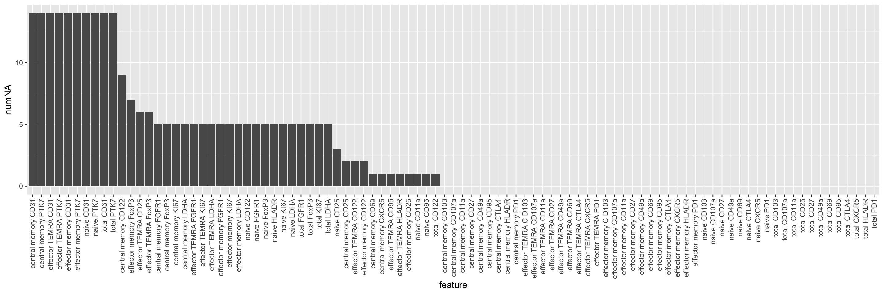

Per-sample

naSum <- group_by(facsTab, sampleID) %>%
    summarise(numNA = sum(is.na(count))) %>%
    arrange(desc(numNA)) %>%
    mutate(sampleID = factor(sampleID, levels = sampleID))
ggplot(naSum, aes(x=sampleID, y=numNA)) +
    geom_bar(stat = "identity") +
    theme(axis.text.x = element_text(angle = 90, hjust = 1, vjust = 0.5))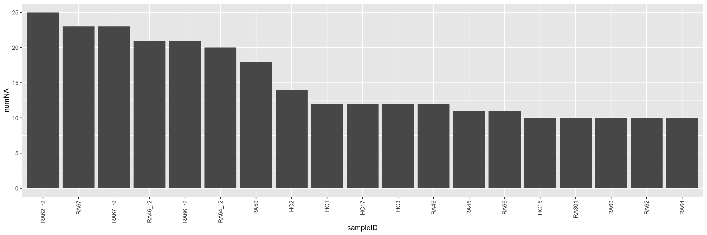

Missing value pattern

missTab <- facsTab %>% mutate(isNA = is.na(count))
ggplot(missTab, aes(x=marker, y=sampleID, fill=isNA)) +
    geom_tile() +
    facet_wrap(~cell, nrow = 1) +
    theme(axis.text.x = element_text(angle = 90, hjust = 1, vjust = 0.5))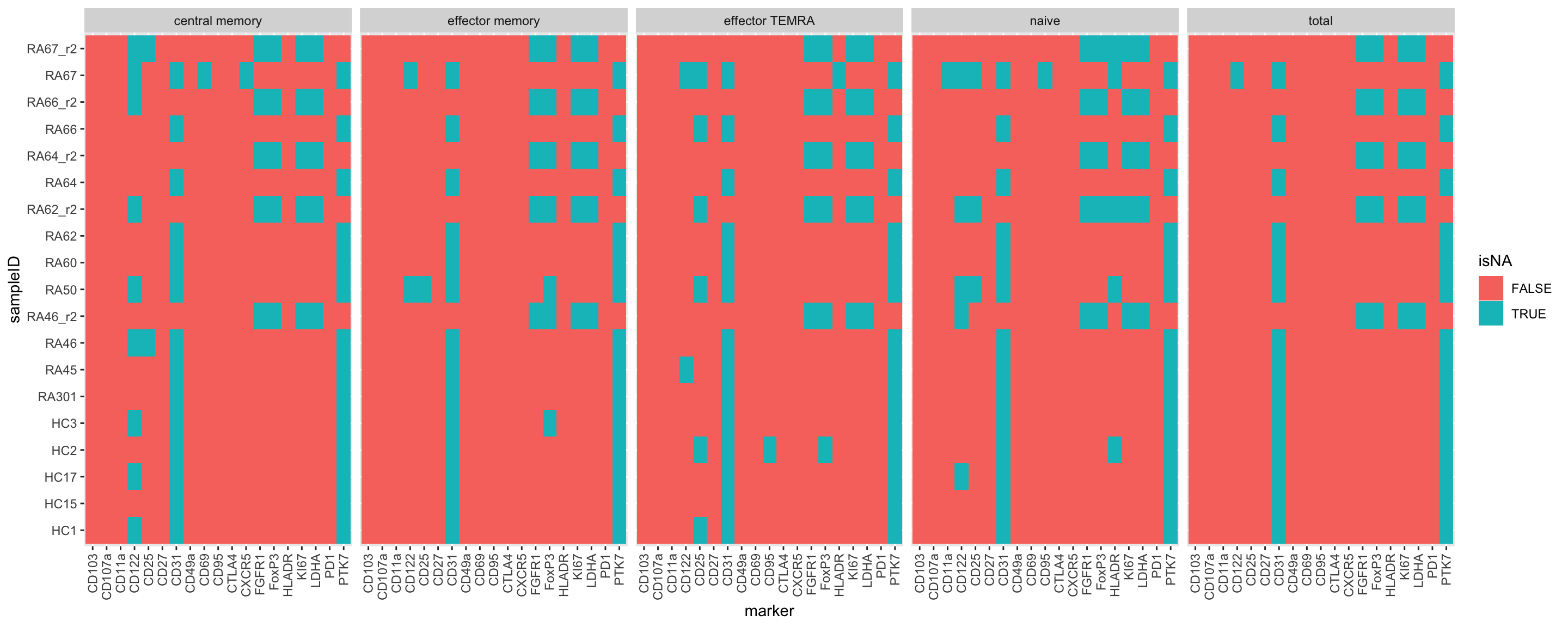

Replicate 2 uses a different panel?

Feature distribution

Per-sample

Raw scale

ggplot(plotTab, aes(x=sampleID, y=count, fill = group)) +
    geom_boxplot() + geom_point() +
    theme(axis.text.x = element_text(angle = 90, hjust=1, vjust =0.5))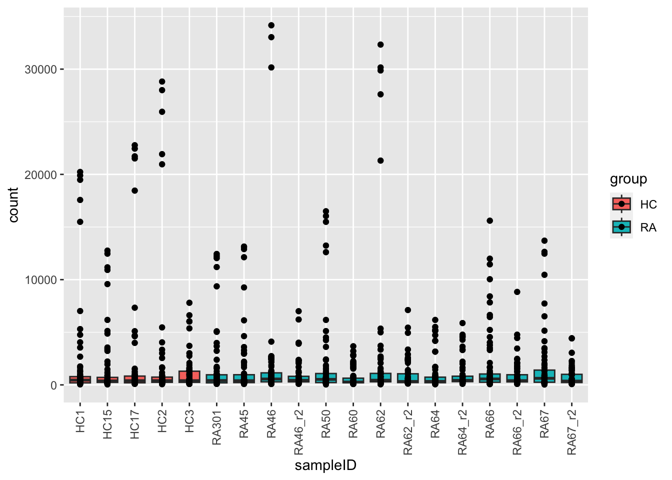

glog transformed

ggplot(plotTab, aes(x=sampleID, y=glog2(count), fill = group)) +
    geom_boxplot() + geom_point() +
    theme(axis.text.x = element_text(angle = 90, hjust=1, vjust =0.5))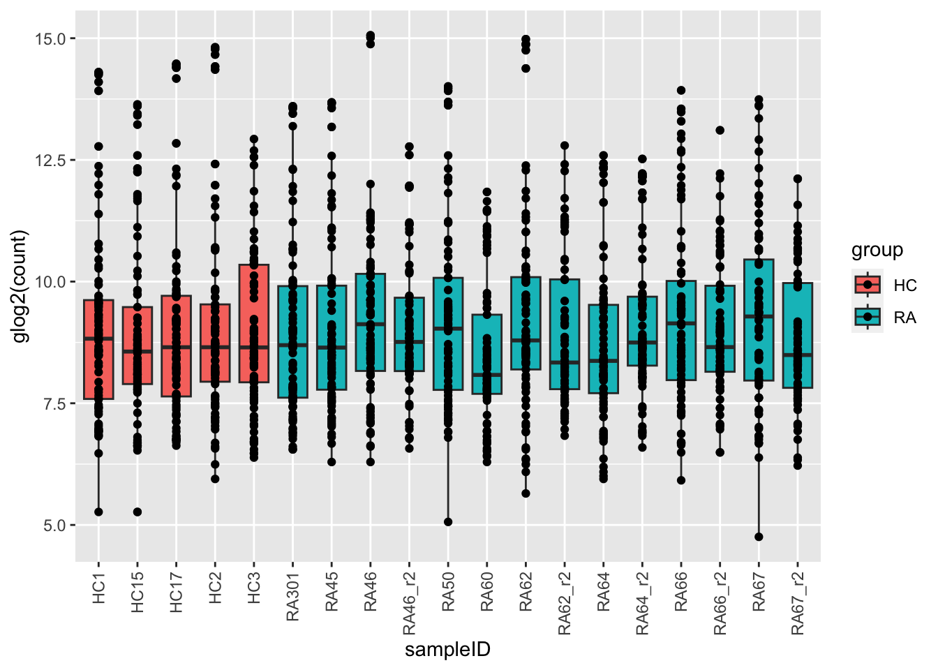

Per feature

Raw scale

ggplot(plotTab, aes(x=feature, y=count)) +
    geom_boxplot() + geom_point(aes(col=group)) +
    theme(axis.text.x = element_text(angle = 90, hjust=1, vjust =0.5))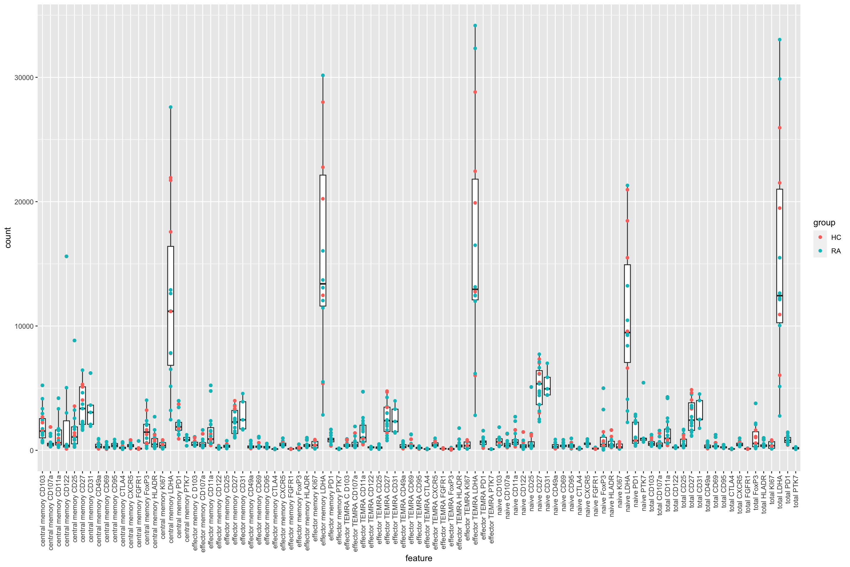

glog transformed

ggplot(plotTab, aes(x=feature, y=glog2(count))) +
    geom_boxplot() + geom_point(aes(col= group))  +
    theme(axis.text.x = element_text(angle = 90, hjust=1, vjust =0.5))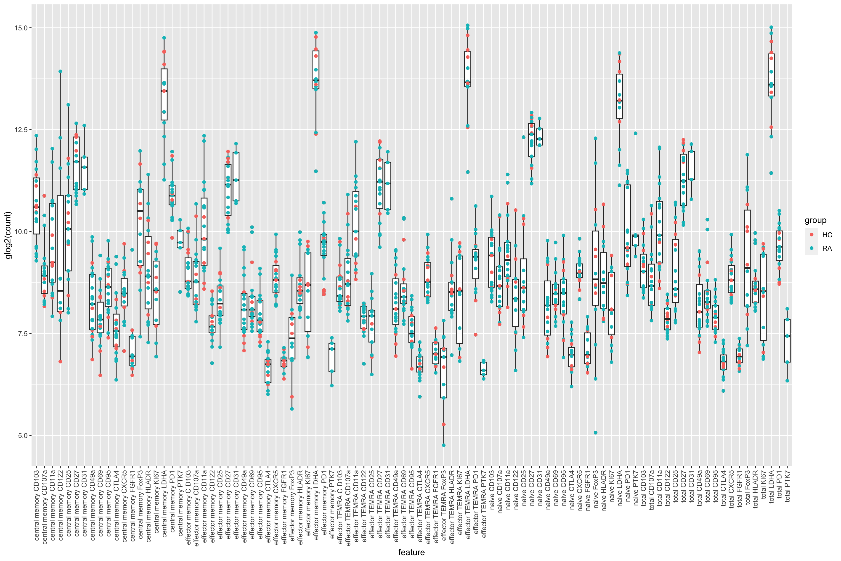

PCA

Raw scale

facsMat <- assay(seFacs)
#only use features with complete measurement
facsMat <- facsMat[complete.cases(facsMat),]
pcRes <- prcomp(t(facsMat), scale. = TRUE, center = TRUE)
plotTab <- pcRes$x %>% as_tibble(rownames = "sampleID") %>%
    mutate(group = seFacs[,sampleID]$group)
ggplot(plotTab, aes(x=PC1, y=PC2, col = group, label = sampleID)) +
    geom_point() +
    geom_text()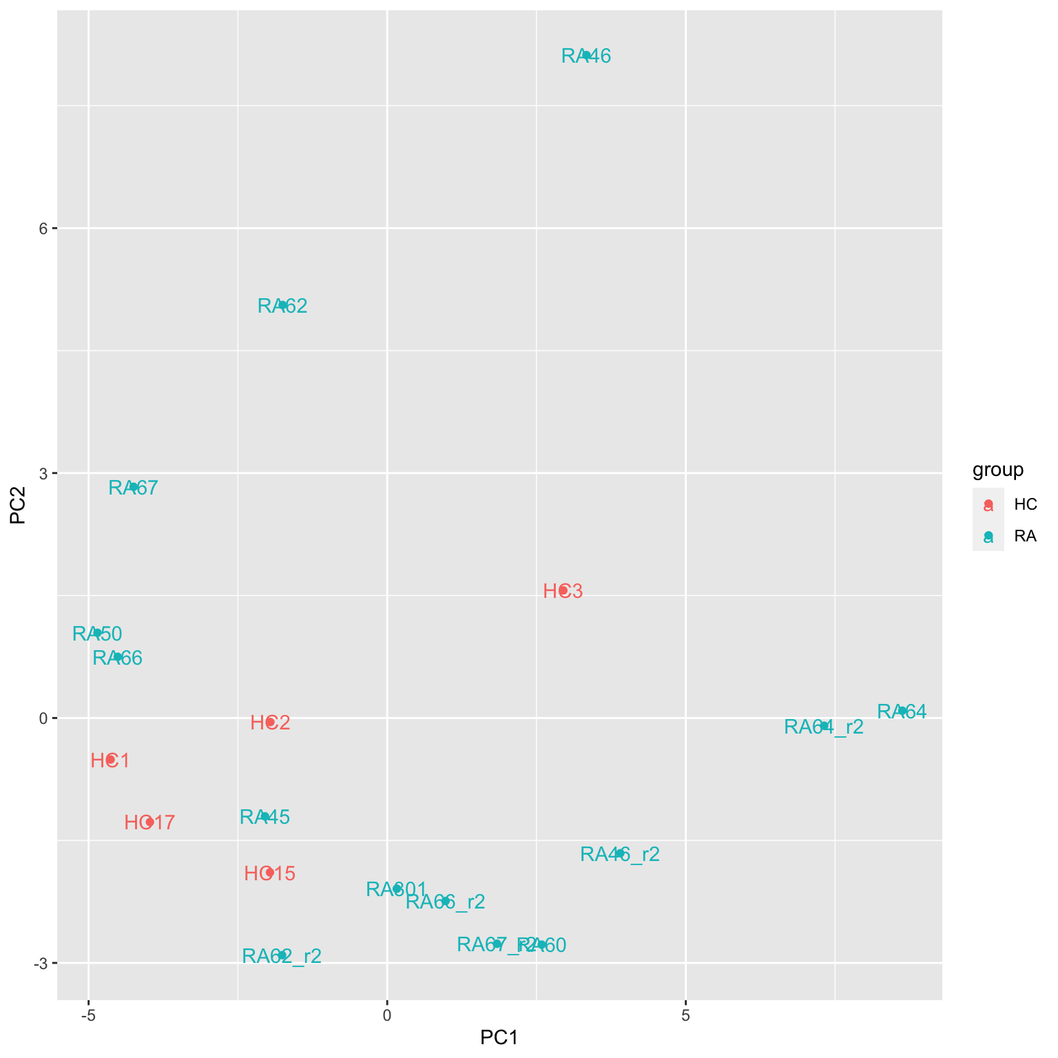

glog transformed

Colored by phenotype

facsMat <- jyluMisc::glog2(facsMat)
pcRes <- prcomp(t(facsMat), scale. = TRUE, center = TRUE)
plotTab <- pcRes$x %>% as_tibble(rownames = "sampleID")  %>%
    mutate(group = seFacs[,sampleID]$group)
ggplot(plotTab, aes(x=PC1, y=PC2, col = group, label = sampleID)) +
    geom_point() +
    geom_text()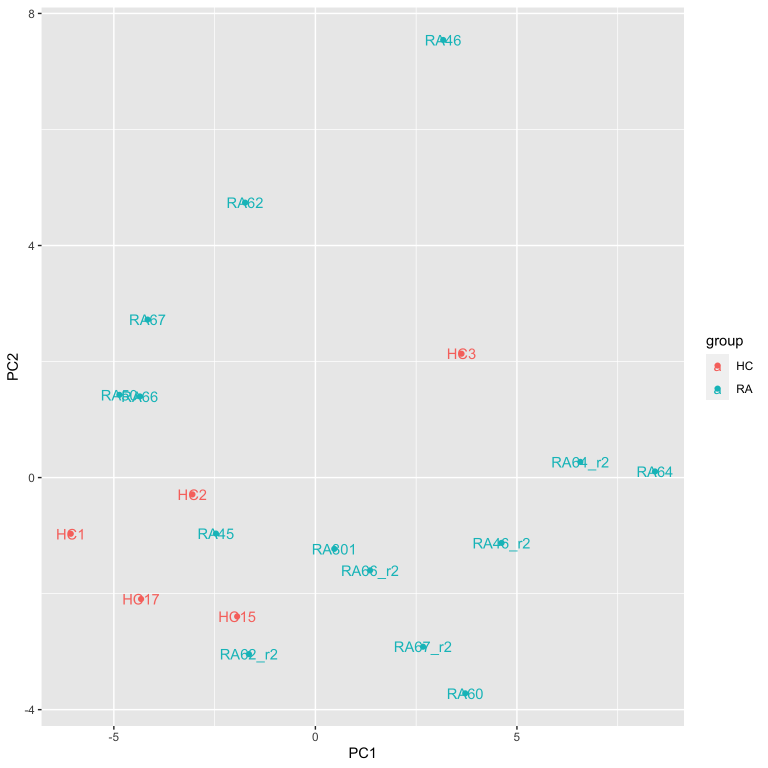

Replicates look very different
Are replicates all measured on a different date?

Compare reproducibility among replicates

repSmp <- unique(filter(facsTab, rep == "r2")$sampleName)
comTab <- filter(facsTab, sampleName %in% repSmp) %>%
    select(feature, sampleName, rep, count) %>%
    mutate(count = glog2(count)) %>%
    pivot_wider(names_from = rep, values_from = count)
ggplot(comTab, aes(x=r1, y=r2)) +
    geom_point() +
    geom_abline(intercept = 0, slope = 1, color = "red")+
    facet_wrap(~sampleName) +
    xlim(-1,15) + ylim(-1,15)

Remove R2 samples

seFacs <- seFacs[,!str_detect(seFacs$sampleID,"r2")]
seFacs$sampleID <- seFacs$sampleName
seFacs$sampleName <- NULL

Remove feature without any measurment

seFacs <- seFacs[rowSums(!is.na(assay(seFacs)))>0,]

Cell population

popTab <- readxl::read_xlsx("../data/Data_2023-02-16/FACS Data MFIs for Junyan.xlsx", sheet = 2) %>%
    pivot_longer(-`...1`, names_to = "sampleName", values_to = "count") %>%
    mutate(sampleName = str_remove(sampleName, "\\.{3}[:digit:]*")) %>%
    dplyr::rename(feature = `...1`) %>%
    group_by(feature, sampleName) %>%
    mutate(rep = seq_along(sampleName)) %>%
    ungroup() %>%
    mutate(rep = paste0("r",rep)) %>%
    mutate(sampleID=ifelse(rep == "r1", sampleName, paste0(sampleName,"_",rep)),
           count = as.numeric(count)) 


popTab <- popTab %>%
    left_join(patTab, by = c(sampleName = "sampleID"))

ggplot(popTab, aes(x=group, y=count, label = sampleID)) +
    geom_boxplot() +
    geom_point(aes(col = group)) +
    ggrepel::geom_text_repel(max.overlaps = Inf) +
    facet_wrap(~feature, scale = "free")

May not be very informative, so it will not be used for multi-omic analysis

Process new DIA Proteomics data received in March, 2024

Read sample metadata

smpMeta <- readxl::read_xlsx("../data/TF0837_results/2023-12-18_SampleSubmission_Kraus_post randomization.xlsx") %>%
  dplyr::rename(id = `Sample Number (same as vial label)`,
                sampleID = `Sample Name`,
                quantStart = "Quantity of Starting Material") %>%
  mutate(quantStart = str_remove(quantStart," lymphocytes")) %>%
  separate(quantStart, into = c("baseN","expN"), sep = "\\*10\\^") %>%
  mutate(quantStart = as.numeric(baseN)*10^as.numeric(expN)) %>%
  select(id, sampleID, quantStart)

Read data table

protTab <- readxl::read_xlsx("../data/TF0837_results/TF0837_filtered_proteinGroups.xlsx") %>%
    select(`PG.ProteinGroups`, `PG.Genes`, contains("PG.Quantity")) %>%
    dplyr::rename(name = "PG.ProteinGroups", symbol = "PG.Genes") %>%
    pivot_longer(-c(name, symbol), names_to = "id", values_to = "count") %>%
    mutate(id = as.numeric(str_extract(id, "(?<=TF0837-)..(?=\\.raw)"))) %>%
    filter(count>0) %>% left_join(smpMeta, by = "id") %>%
    left_join(patTab, by = "sampleID")
idMap <- unique(protTab$name)
idMap <- structure(paste0("prot",seq_along(idMap)), names = idMap)
protTab <- mutate(protTab, ID = idMap[name])

Choose the first symbol if multiple symbols are present in the symbol column

# Get the last symbol of a protein that has multiple gene symbols
getOneSymbol <- function(Gene) {
    outStr <- sapply(Gene, function(x) {
        sp <- str_split(x, ";")[[1]]
        sp[length(sp)]
    })
    names(outStr) <- NULL
    outStr
}
protTab$symbol <- getOneSymbol(protTab$symbol)

#only keep proteins with symbols
protTab <- filter(protTab, !symbol %in% c("",NA), !str_detect(symbol, "SWISS-PROT"))

Created summarised experiment

seDIA <- jyluMisc::tidyToSum(protTab, "ID", "sampleID","count",
                               annoRow = c("ID","name","symbol"),
                               annoCol = c(colnames(patTab),"quantStart"))

Some samples don’t have the group information, but this can be determined by the sample name

seDIA$group <- ifelse(is.na(seDIA$group), ifelse(str_detect(colnames(seDIA),"HC"), "HC", "RA"), seDIA$group)

QA

Data completeness per sample

countMat <- assay(seDIA)
plotTab <- tibble(sample = colnames(seDIA), 
                  perNA = colSums(is.na(countMat))/nrow(countMat),
                  startQuant = seDIA$quantStart)
ggplot(plotTab, aes(x=sample, y=1-perNA)) +
    geom_bar(stat = "identity", aes(fill = startQuant)) +
    ylab("completeness") +
    theme(axis.text.x = element_text(angle = 90, hjust = 1, vjust=0))

Plot a cumulative curve of missing value cut-off and remaining number of features

missRate <- tibble(id = rownames(countMat),
                   rate = rowSums(is.na(countMat))/ncol(countMat))
cumTab <- lapply(seq(0,1,0.05), function(cutRate) {
    tibble(cut= cutRate,
           per = sum(missRate$rate <= cutRate)/nrow(missRate))
} ) %>%
    bind_rows()
ggplot(cumTab, aes(x=cut,y=per)) +
    geom_line() +
    xlab("Allowed missing value rate") +
    ylab("Percentage of remaining features")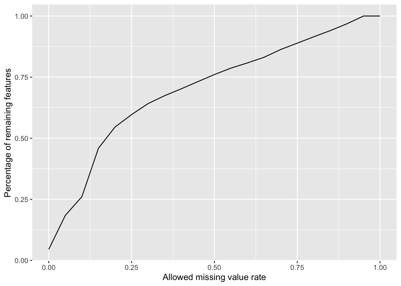

Missing value heatmap to check missing value structure

Visualize the missing value pattern

DEP::plot_missval(seDIA)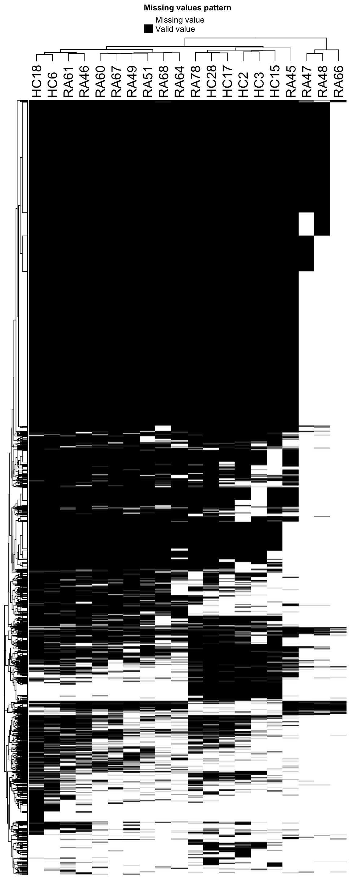

Looks pretty sparse, maybe due to the DDA data aquisition method

Keep proteins detected in at least half of the sample (missing rate <= 0.5)

protFilt <- seDIA[filter(missRate, rate <=0.5)$id,]
dim(protFilt)

[1] 5292   20

Data distribution

countMat <- assay(protFilt)
countTab <- countMat %>% as_tibble(rownames = "id") %>% 
    pivot_longer(-id) %>%
    filter(!is.na(value)) %>%
    mutate(log2Val = log2(value))

ggplot(countTab, aes(x=name, y=log2Val)) +
    geom_boxplot() + geom_point()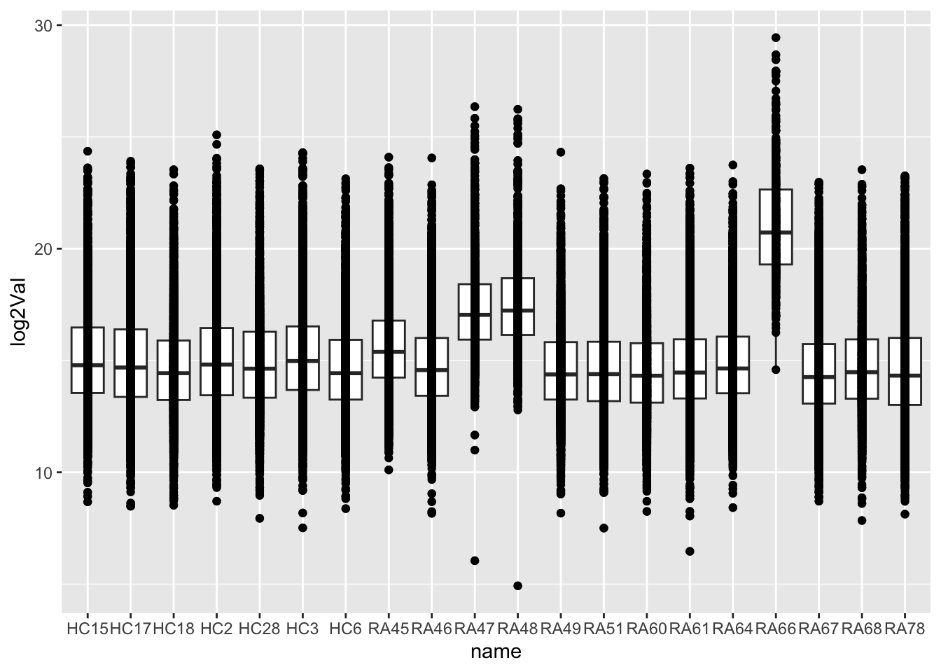

Imputation and normalization

Vst

protMat <- assay(protFilt)
fitVsn <- vsn::vsnMatrix(protMat)
normMat <- vsn::predict(fitVsn, newdata = protMat)
protNorm <- protFilt
assay(protNorm) <- normMat

Imputation

protImp <- DEP::impute(protNorm, "QRILC")
assays(protFilt)[["norm"]] <- normMat
assays(protFilt)[["imputed"]] <- assay(protImp)
rowData(protFilt) <- rowData(protImp)

Distribution after normalizaiton

countMat <- assays(protFilt)[["imputed"]]
countTab <- countMat %>% as_tibble(rownames = "id") %>% 
    pivot_longer(-id) %>%
    filter(!is.na(value))
ggplot(countTab, aes(x=name, y=value)) +
    geom_boxplot() + geom_point()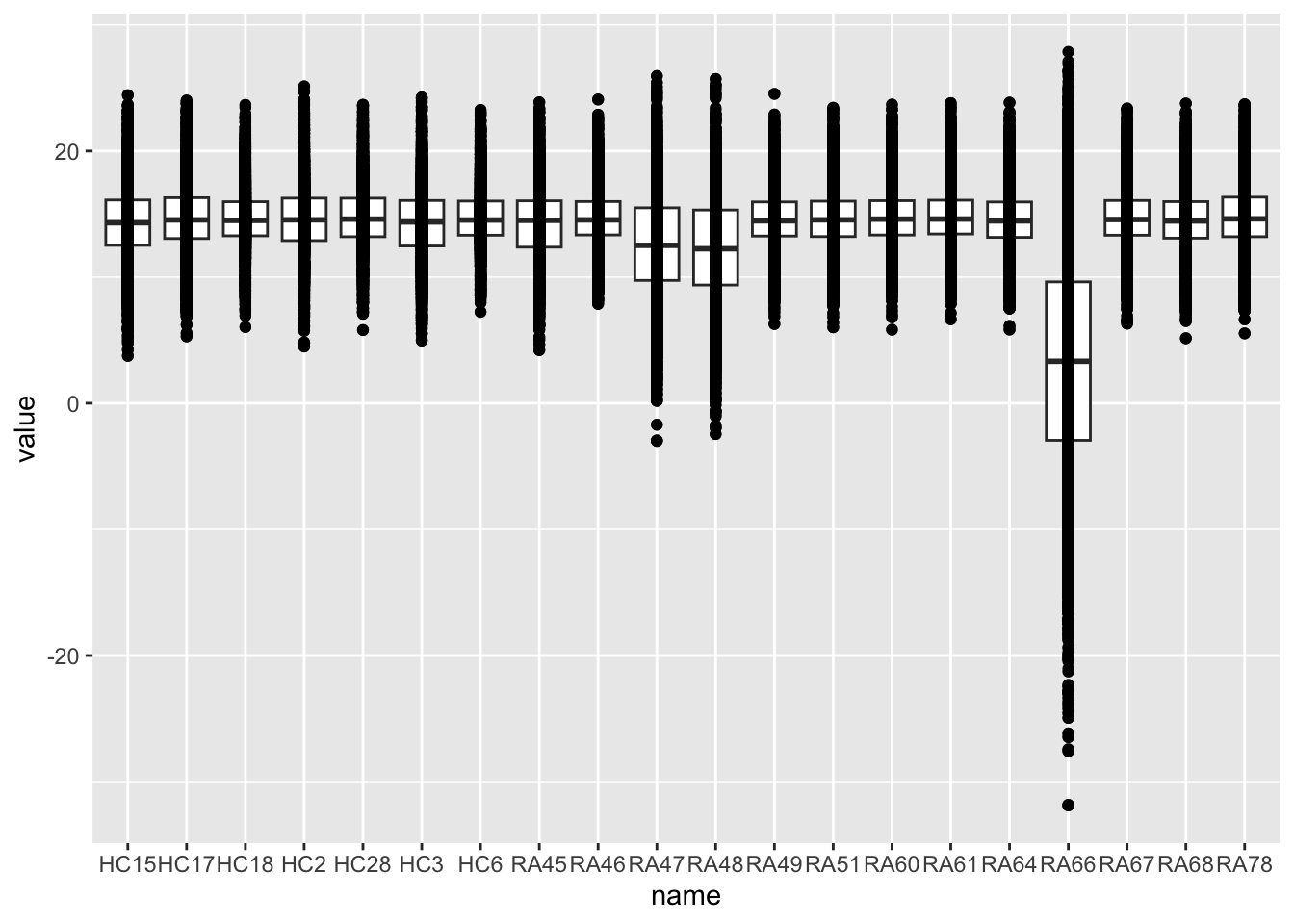

Mean versus variant plot

plotTab <- tibble(meanVal = rowMeans(countMat),
                  var = apply(countMat, 1, var))
ggplot(plotTab, aes(x=meanVal,y=var)) +
    geom_point()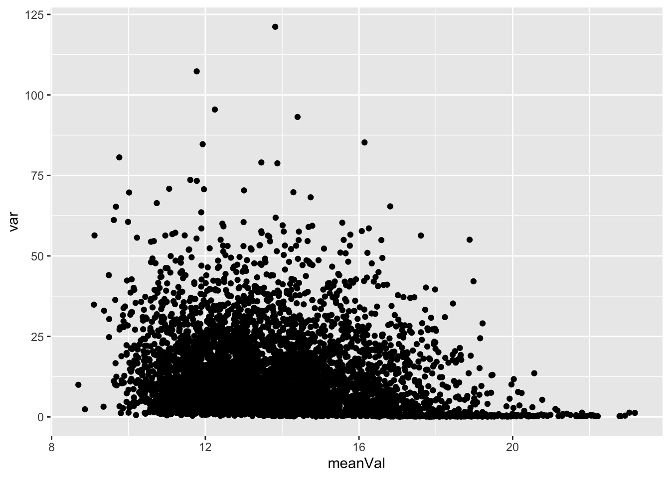

Heatmap visualization

library(pheatmap)
#select top 1000 most variant
colAnno <- colData(protFilt) %>% data.frame()
colAnno <- colAnno[,c("Gender","group","quantStart")]
#colAnno[["sampleName"]] <- NULL
plotMat <- countMat[order(plotTab$var, decreasing = TRUE)[1:1000],]
pheatmap(plotMat, show_rownames = FALSE, scale = "row", 
         annotation_col = colAnno,
         clustering_method = "ward.D2")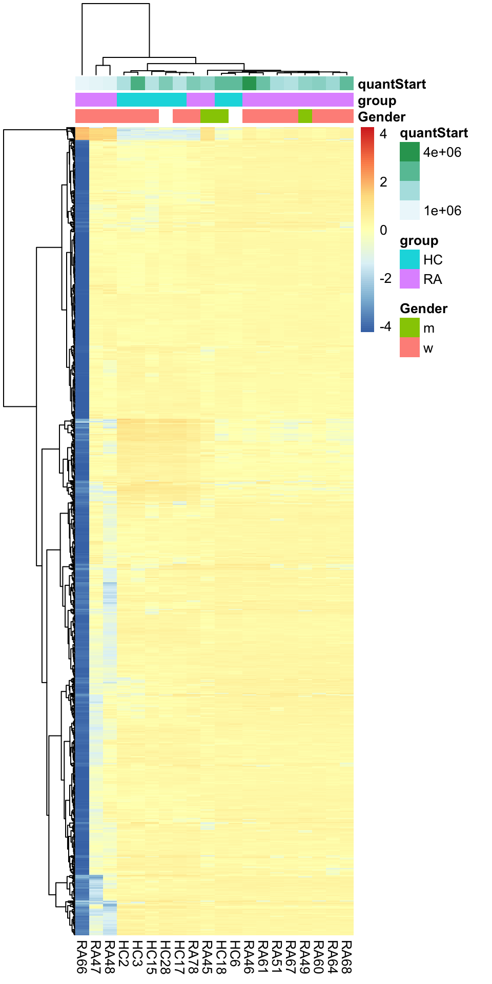

Buffer composition and startQuant could be potential counfunding factor

PCA

prRes <- prcomp(t(plotMat), scale. = FALSE, center = TRUE)
plotTab <- prRes$x %>% as_tibble(rownames = "sampleID") %>%
    left_join(as_tibble(colAnno, rownames = "sampleID"))
ggplot(plotTab, aes(x=PC1, y=PC2, col = group)) +
    geom_point() +
    ggrepel::geom_text_repel(aes(label = sampleID))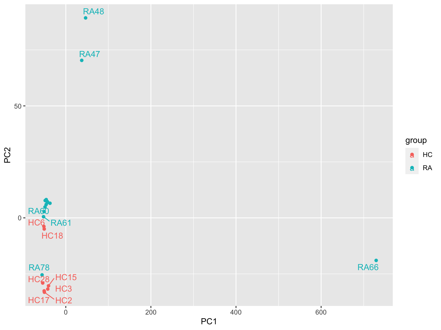

RA66, RA47 and RA48 looks like an outlier

Remove three potential outliers and redo the preprocessing

Subset

diaSub <- seDIA[,! seDIA$sampleID %in% c("RA66","RA47","RA48")]

#remove proteins with more than 50% missing values
diaSub <- diaSub[rowSums(is.na(assay(diaSub)))/ncol(diaSub)<=0.5,]
dim(diaSub)

[1] 5450   17

Vst

protMat <- assay(diaSub)
fitVsn <- vsn::vsnMatrix(protMat)
normMat <- vsn::predict(fitVsn, newdata = protMat)
protNorm <- diaSub
assay(protNorm) <- normMat

Imputation

protImp <- DEP::impute(protNorm, "bpca")
assays(diaSub)[["norm"]] <- normMat
assays(diaSub)[["imputed"]] <- assay(protImp)

Distribution after normalizaiton

countMat <- assays(diaSub)[["norm"]]
countTab <- countMat %>% as_tibble(rownames = "id") %>% 
    pivot_longer(-id) %>%
    filter(!is.na(value))
ggplot(countTab, aes(x=name, y=value)) +
    geom_boxplot() + geom_point()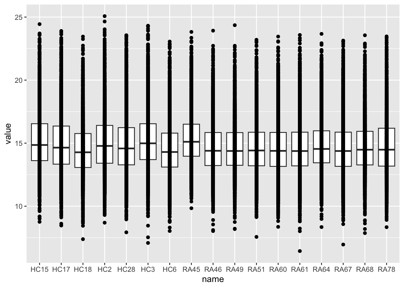

Redo pca

Color by group

plotMat <- assays(diaSub)[["imputed"]]
prRes <- prcomp(t(plotMat), scale. = TRUE, center = TRUE)
plotTab <- prRes$x %>% as_tibble(rownames = "sampleID") %>%
    left_join(as_tibble(colAnno, rownames = "sampleID"))
ggplot(plotTab, aes(x=PC1, y=PC2, col = group)) +
    geom_point() +
    ggrepel::geom_text_repel(aes(label = sampleID))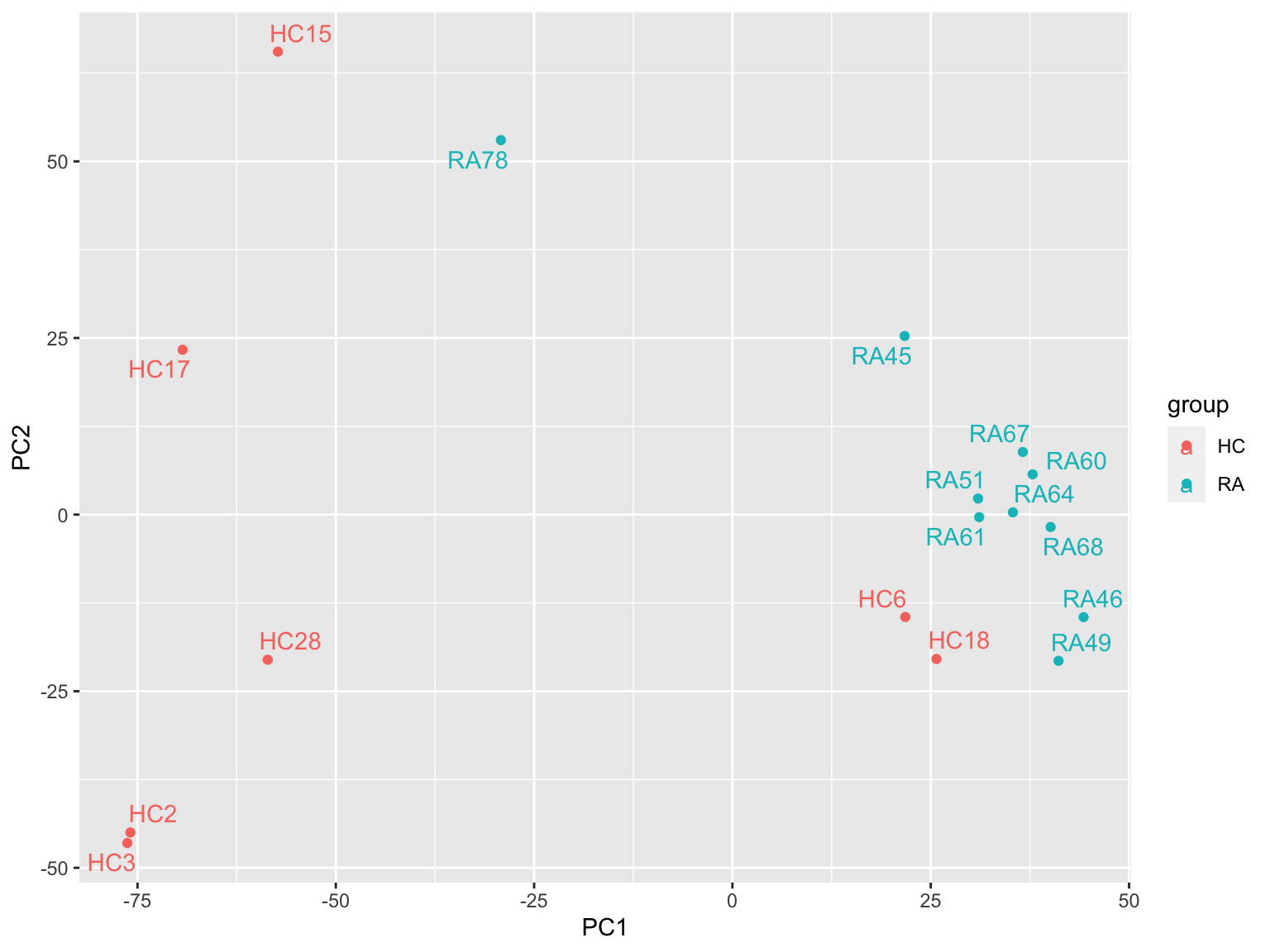

Looks better.

Color by quantStart

plotMat <- assays(diaSub)[["imputed"]]
prRes <- prcomp(t(plotMat), scale. = TRUE, center = TRUE)
plotTab <- prRes$x %>% as_tibble(rownames = "sampleID") %>%
    left_join(as_tibble(colAnno, rownames = "sampleID"))
ggplot(plotTab, aes(x=PC1, y=PC2, col = quantStart)) +
    geom_point() +
    ggrepel::geom_text_repel(aes(label = sampleID))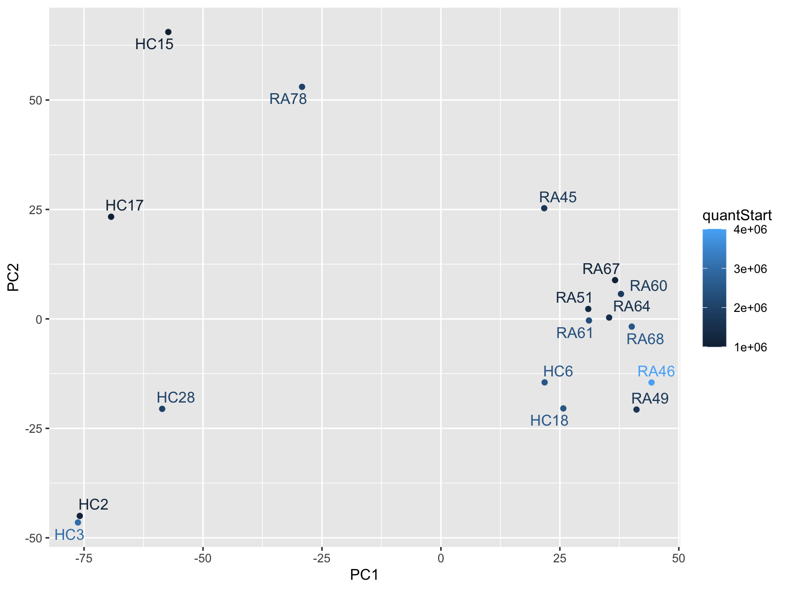

Assemble Multi-assay experiment object

library(MultiAssayExperiment)
maeObj <- MultiAssayExperiment(experiments = list(Metabolism = seMeta, Proteome = protSub, Proteome_DIA = diaSub,
                                                  Phosphoproteome = phosSub, PhosRatio = seRatio,
                                                  Methylation = methMat, FACS = seFacs),
                                colData = patTab %>% column_to_rownames("sampleID") %>% data.frame())
save(maeObj, file = "../output/maeObj.RData")

sessionInfo()

R version 4.2.0 (2022-04-22)
Platform: x86_64-apple-darwin17.0 (64-bit)
Running under: macOS Big Sur/Monterey 10.16

Matrix products: default
BLAS:   /Library/Frameworks/R.framework/Versions/4.2/Resources/lib/libRblas.0.dylib
LAPACK: /Library/Frameworks/R.framework/Versions/4.2/Resources/lib/libRlapack.dylib

locale:
[1] en_US.UTF-8/en_US.UTF-8/en_US.UTF-8/C/en_US.UTF-8/en_US.UTF-8

attached base packages:
[1] stats4    stats     graphics  grDevices utils     datasets  methods  
[8] base     

other attached packages:
 [1] MultiAssayExperiment_1.22.0 pheatmap_1.0.12            
 [3] forcats_0.5.1               stringr_1.4.1              
 [5] dplyr_1.1.4.9000            purrr_0.3.4                
 [7] readr_2.1.2                 tidyr_1.2.0                
 [9] tibble_3.2.1                ggplot2_3.4.1              
[11] tidyverse_1.3.2             SummarizedExperiment_1.26.1
[13] GenomicRanges_1.48.0        GenomeInfoDb_1.32.2        
[15] IRanges_2.30.0              S4Vectors_0.34.0           
[17] MatrixGenerics_1.8.1        matrixStats_0.62.0         
[19] jyluMisc_0.1.5              vsn_3.64.0                 
[21] Biobase_2.56.0              BiocGenerics_0.42.0        

loaded via a namespace (and not attached):
  [1] DEP_1.18.0             utf8_1.2.4             shinydashboard_0.7.2  
  [4] gmm_1.6-6              tidyselect_1.2.1       RSQLite_2.2.15        
  [7] AnnotationDbi_1.58.0   htmlwidgets_1.5.4      grid_4.2.0            
 [10] BiocParallel_1.30.3    norm_1.0-10.0          maxstat_0.7-25        
 [13] munsell_0.5.0          codetools_0.2-18       preprocessCore_1.58.0 
 [16] DT_0.23                withr_3.0.0            colorspace_2.0-3      
 [19] highr_0.9              knitr_1.39             rstudioapi_0.13       
 [22] ggsignif_0.6.3         mzID_1.34.0            labeling_0.4.2        
 [25] git2r_0.30.1           slam_0.1-50            GenomeInfoDbData_1.2.8
 [28] KMsurv_0.1-5           bit64_4.0.5            farver_2.1.1          
 [31] rprojroot_2.0.3        vctrs_0.6.5            generics_0.1.3        
 [34] TH.data_1.1-1          xfun_0.31              sets_1.0-21           
 [37] R6_2.5.1               doParallel_1.0.17      clue_0.3-61           
 [40] MsCoreUtils_1.8.0      bitops_1.0-7           cachem_1.0.6          
 [43] fgsea_1.22.0           DelayedArray_0.22.0    assertthat_0.2.1      
 [46] promises_1.2.0.1       scales_1.2.0           multcomp_1.4-19       
 [49] googlesheets4_1.0.0    gtable_0.3.0           Cairo_1.6-0           
 [52] affy_1.74.0            sandwich_3.0-2         workflowr_1.7.0       
 [55] rlang_1.1.3            genefilter_1.78.0      mzR_2.30.0            
 [58] GlobalOptions_0.1.2    splines_4.2.0          rstatix_0.7.0         
 [61] gargle_1.2.0           impute_1.70.0          broom_1.0.0           
 [64] BiocManager_1.30.18    yaml_2.3.5             abind_1.4-5           
 [67] modelr_0.1.8           crosstalk_1.2.0        backports_1.4.1       
 [70] httpuv_1.6.6           tools_4.2.0            relations_0.6-12      
 [73] affyio_1.66.0          ellipsis_0.3.2         gplots_3.1.3          
 [76] jquerylib_0.1.4        RColorBrewer_1.1-3     MSnbase_2.22.0        
 [79] plyr_1.8.7             Rcpp_1.0.9             visNetwork_2.1.0      
 [82] zlibbioc_1.42.0        RCurl_1.98-1.7         ggpubr_0.4.0          
 [85] GetoptLong_1.0.5       cowplot_1.1.1          zoo_1.8-10            
 [88] ggrepel_0.9.1          haven_2.5.0            cluster_2.1.3         
 [91] exactRankTests_0.8-35  fs_1.5.2               magrittr_2.0.3        
 [94] magick_2.7.3           data.table_1.14.8      circlize_0.4.15       
 [97] reprex_2.0.1           survminer_0.4.9        pcaMethods_1.88.0     
[100] googledrive_2.0.0      mvtnorm_1.1-3          ProtGenerics_1.28.0   
[103] hms_1.1.1              shinyjs_2.1.0          mime_0.12             
[106] evaluate_0.15          xtable_1.8-4           XML_3.99-0.10         
[109] readxl_1.4.0           gridExtra_2.3          shape_1.4.6           
[112] compiler_4.2.0         KernSmooth_2.23-20     ncdf4_1.19            
[115] crayon_1.5.2           htmltools_0.5.4        later_1.3.0           
[118] tzdb_0.3.0             lubridate_1.8.0        DBI_1.1.3             
[121] dbplyr_2.2.1           ComplexHeatmap_2.12.1  tmvtnorm_1.5          
[124] MASS_7.3-58            Matrix_1.5-4           car_3.1-0             
[127] cli_3.6.2              imputeLCMD_2.1         marray_1.74.0         
[130] parallel_4.2.0         igraph_1.3.4           pkgconfig_2.0.3       
[133] km.ci_0.5-6            piano_2.12.0           MALDIquant_1.21       
[136] xml2_1.3.3             foreach_1.5.2          annotate_1.74.0       
[139] bslib_0.4.1            XVector_0.36.0         drc_3.0-1             
[142] rvest_1.0.2            digest_0.6.30          Biostrings_2.64.0     
[145] rmarkdown_2.14         cellranger_1.1.0       fastmatch_1.1-3       
[148] survMisc_0.5.6         shiny_1.7.4            gtools_3.9.3          
[151] rjson_0.2.21           lifecycle_1.0.4        jsonlite_1.8.3        
[154] carData_3.0-5          limma_3.52.2           fansi_1.0.6           
[157] pillar_1.9.0           lattice_0.20-45        KEGGREST_1.36.3       
[160] fastmap_1.1.0          httr_1.4.3             plotrix_3.8-2         
[163] survival_3.4-0         glue_1.7.0             png_0.1-7             
[166] iterators_1.0.14       bit_4.0.4              stringi_1.7.8         
[169] sass_0.4.2             blob_1.2.3             memoise_2.0.1         
[172] caTools_1.18.2

Process each omics data of T cells

Junyan Lu

Load libraries

Load sample annotations

Process the the new metabolic table

QC

Feature distribution

Per-sample

Per feature

PCA

Raw scale

glog transformed

Process Proteomics data

Read data table

QA

Data completeness per sample

Data distribution

Imputation and normalization

Heatmap visualization

PCA

Remove one potential outlier, RA62 and redo the preprocessing

Redo pca

Phospho-proteomics

Read data table

QA

Data completeness per sample

Data distribution

Imputation and normalization

Heatmap visualization

PCA

Remove one potential outlier, RA62 and redo preprocessing

Redo pca

Phosphorylation normalized by protein expression

Methylation data

FACS data

QC

Measing value count

Per-feature

Per-sample

Missing value pattern

Feature distribution

Per-sample

Per feature

PCA

Raw scale

glog transformed

Compare reproducibility among replicates

Remove R2 samples

Cell population

Process new DIA Proteomics data received in March, 2024

Read data table

QA

Data completeness per sample

Data distribution

Imputation and normalization

Heatmap visualization

PCA

Remove three potential outliers and redo the preprocessing

Redo pca

Assemble Multi-assay experiment object