Last updated: 2024-11-25

Checks: 4 2

Knit directory: RA_Tcell_omics/analysis/

This reproducible R Markdown analysis was created with workflowr (version 1.7.0). The Checks tab describes the reproducibility checks that were applied when the results were created. The Past versions tab lists the development history.

Environment: empty

Great job! The global environment was empty. Objects defined in the global environment can affect the analysis in your R Markdown file in unknown ways. For reproduciblity it’s best to always run the code in an empty environment.

Seed: set.seed(20221110)

The command set.seed(20221110) was run prior to running the code in the R Markdown file. Setting a seed ensures that any results that rely on randomness, e.g. subsampling or permutations, are reproducible.

Session information: recorded

Great job! Recording the operating system, R version, and package versions is critical for reproducibility.

Cache: detected

The following chunks had caches available:

unnamed-chunk-10
unnamed-chunk-14
unnamed-chunk-15
unnamed-chunk-21
unnamed-chunk-22
unnamed-chunk-32
unnamed-chunk-9

To ensure reproducibility of the results, delete the cache directory singleOmic_analysis_cache and re-run the analysis. To have workflowr automatically delete the cache directory prior to building the file, set delete_cache = TRUE when running wflow_build() or wflow_publish().

File paths: relative

Great job! Using relative paths to the files within your workflowr project makes it easier to run your code on other machines.

Repository version: no version control

Tracking code development and connecting the code version to the results is critical for reproducibility. To start using Git, open the Terminal and type git init in your project directory.

This project is not being versioned with Git. To obtain the full reproducibility benefits of using workflowr, please see ?wflow_start.

Load libraries

Load processed data

load("../output/maeObj.RData")

Analysis of metabolomic data

seMeta <- maeObj[["Metabolism"]]
metaMat <- assay(seMeta)
metaTab <- sumToTidy(seMeta)

Features and numbers

dim(seMeta)

[1] 65 36

Visualize overall data distribution

Per sample

ggplot(metaTab, aes(x=colID, y=glog(count))) +
    geom_boxplot() + geom_point(aes(col = group)) +
    theme(axis.text = element_text(angle = 90, hjust = 1, vjust = 0.5))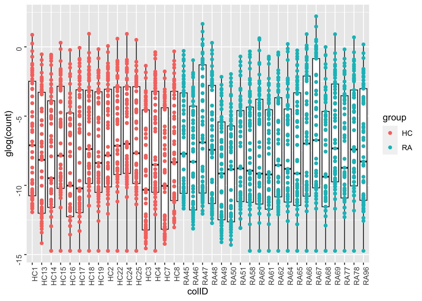

Color by experiment date

ggplot(metaTab, aes(x=colID, y=glog(count))) +
    geom_boxplot() + geom_point(aes(col = dateMeta)) +
    theme(axis.text = element_text(angle = 90, hjust = 1, vjust = 0.5))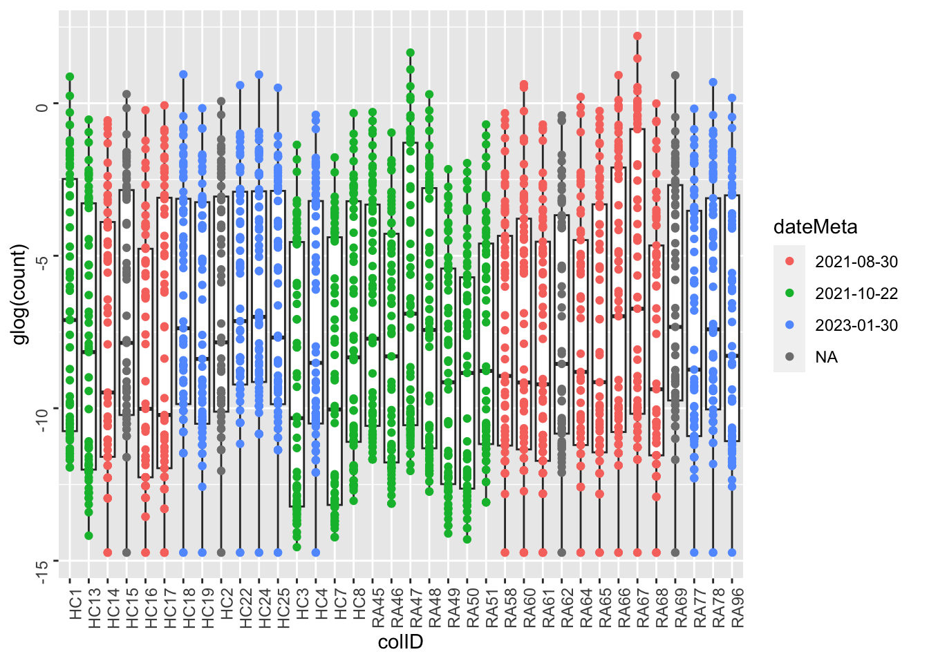

Per metabolite

ggplot(metaTab, aes(x=metabolite, y=glog(count))) +
    geom_boxplot() + geom_point(aes(col = group)) +
    theme(axis.text = element_text(angle = 90, hjust = 1, vjust = 0.5))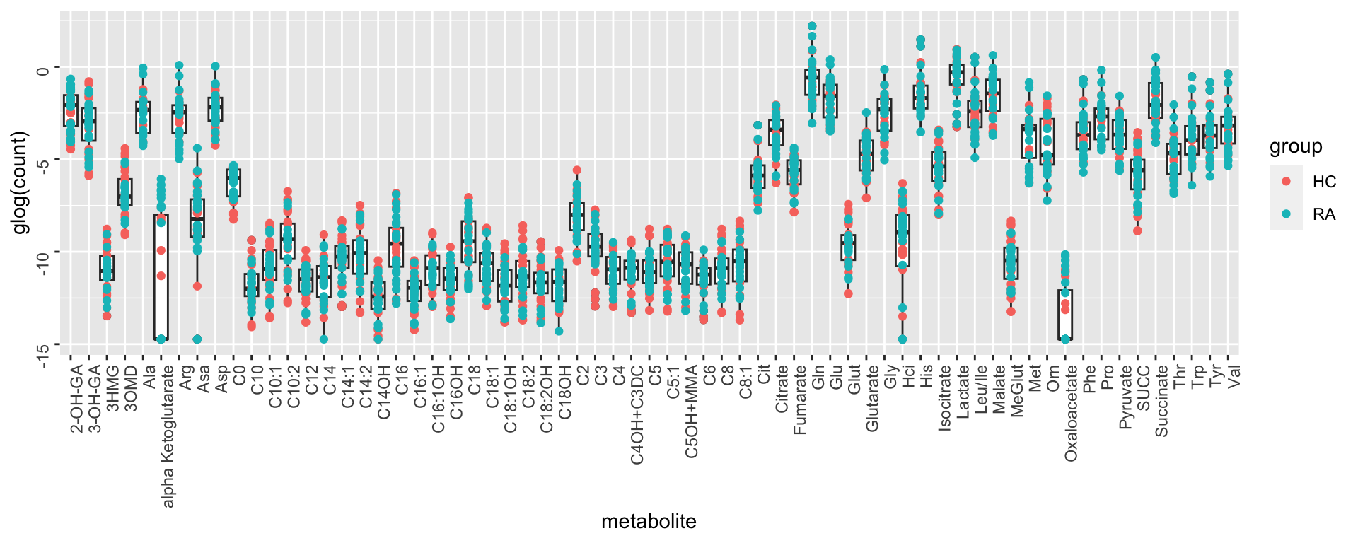

The abundance of different metabolites are very different. Transformation and Normalization may not be needed actually

PCA

By group

metaMat.scale <- glog(metaMat)
pcRes <- prcomp(t(metaMat.scale), scale. = TRUE, center = TRUE)$x
plotTab <- as_tibble(pcRes, rownames = "colID") %>%
    left_join(as.tibble(colData(seMeta), rownames = "colID"))
   
ggplot(plotTab, aes(x=PC1, y=PC2, col = group)) +
    geom_point()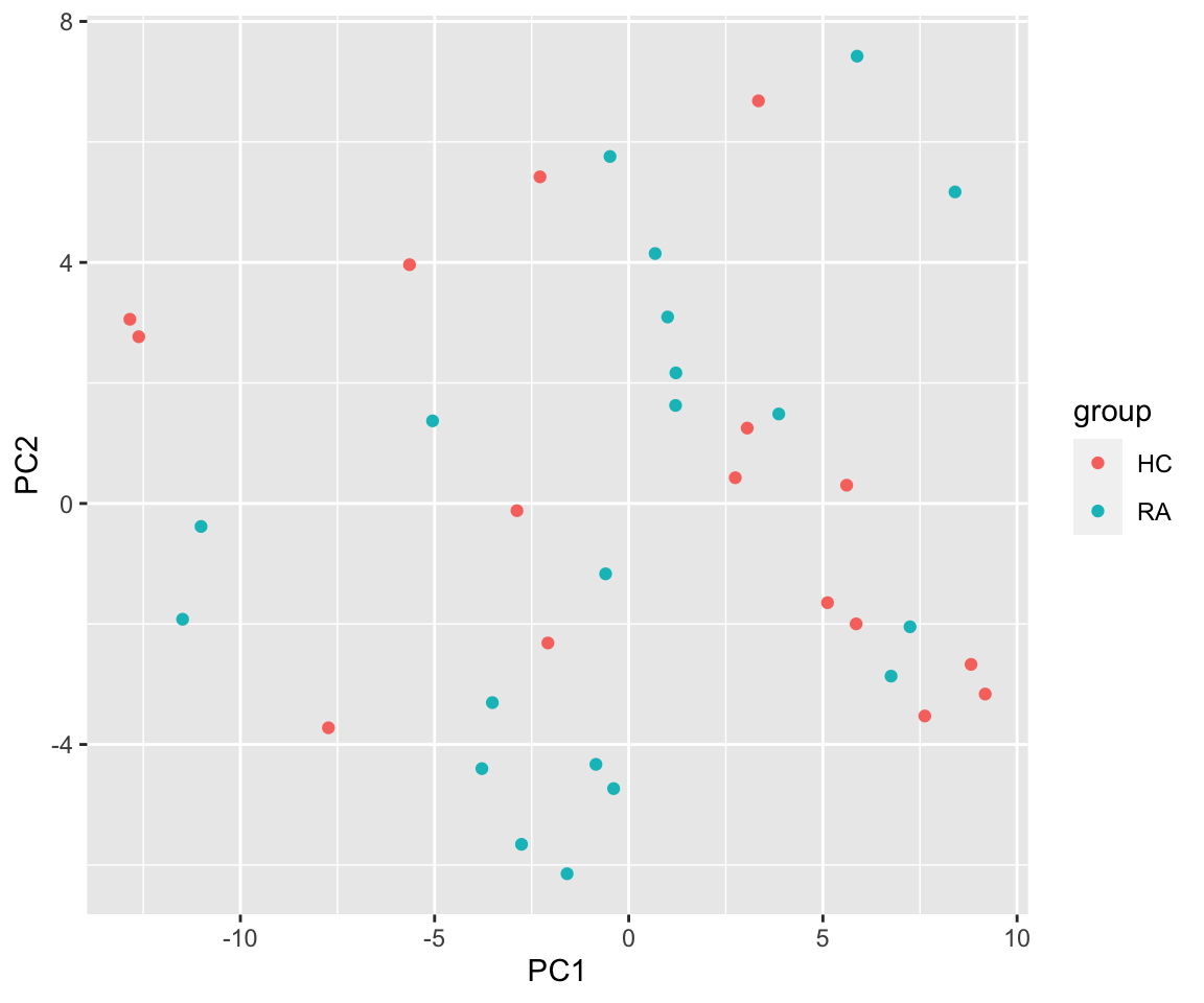

By date

metaMat.scale <- glog(metaMat)
pcRes <- prcomp(t(metaMat.scale), scale. = TRUE, center = TRUE)$x
plotTab <- as_tibble(pcRes, rownames = "colID") %>%
    left_join(as.tibble(colData(seMeta), rownames = "colID"))
   
ggplot(plotTab, aes(x=PC1, y=PC2, col = dateMeta)) +
    geom_point()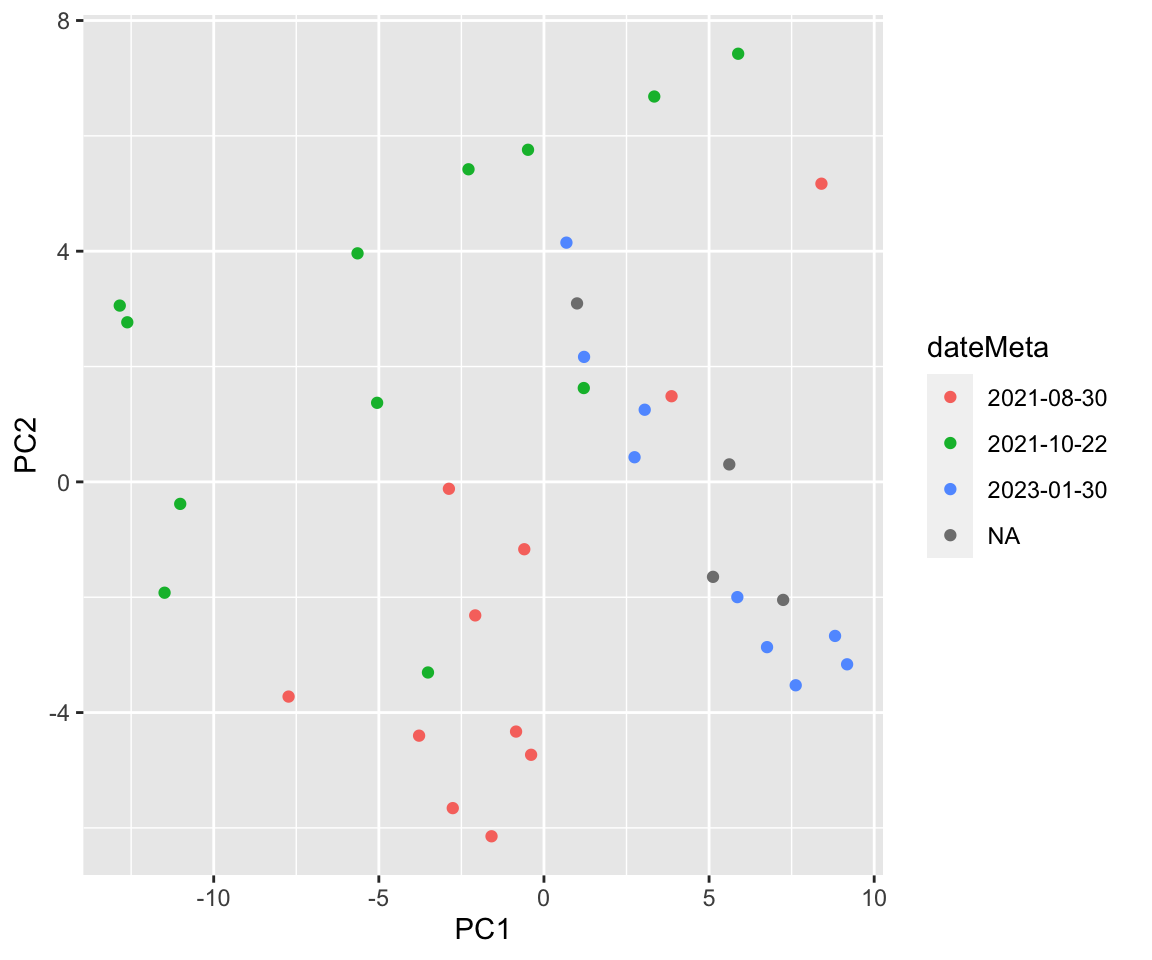

There are potentially some batch effect in the metabolic dataset

table(seMeta$group, seMeta$dateMeta)

    
     2021-08-30 2021-10-22 2023-01-30
  HC          3          5          6
  RA          8          7          3

Differential abundance test

With correction for batch effect. Two samples do not have date information

seMetaSub <- seMeta[,!is.na(seMeta$dateMeta)]
#assay(seMetaSub) <- glog(assay(seMetaSub))
assays(seMetaSub)[["combat"]] <- sva::ComBat(assay(seMetaSub), batch = seMetaSub$dateMeta)

Found 2 genes with uniform expression within a single batch (all zeros); these will not be adjusted for batch.

library(limma)
metaMat <- assays(seMetaSub)[["combat"]]
designMat <- model.matrix(~group, data = colData(seMetaSub))
lmFit <- lmFit(metaMat, design = designMat)
fit2 <- eBayes(lmFit)
resTab <- topTable(fit2, number = Inf) %>%
    as_tibble(rownames = "metabolite")
hist(resTab$P.Value)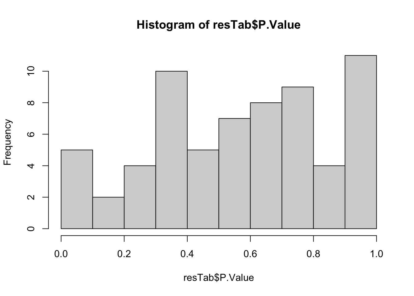

Plot significant associations

pList <- lapply(seq(nrow(filter(resTab, P.Value <= 0.1))), function(i) {
    rec <- resTab[i,]
    plotTab <- filter(metaTab, metabolite == rec$metabolite) %>%
      mutate(group=ifelse(group == "HC","Control",group))
    #plotTab <- tibble(colID = colnames(metaMat),
    #                  count = metaMat[rec$metabolite,]) %>%
    #  mutate(group = seMeta[,colID]$group)
    ggplot(plotTab, aes(x=group, y=count)) + 
        geom_boxplot(outlier.shape = NA, width =0.3) + 
        ggbeeswarm::geom_quasirandom(aes(color = group), size=3, width = 0.3) +
        ggtitle(sprintf("%s\n(P=%s)",rec$metabolite,formatC(rec$P.Value,digits = 2))) +
        scale_color_manual(values =c(Control = "blue", RA = "red")) +
        theme_classic() +
        theme(legend.position = "none",
              axis.text = element_text(face = "bold", size=14), axis.title = element_text(face = "bold",size=14),
              plot.title = element_text(hjust=.5, face = "bold")) +
      ylab("log (abundance)") + xlab("")
})
cowplot::plot_grid(plotlist = pList,ncol=3)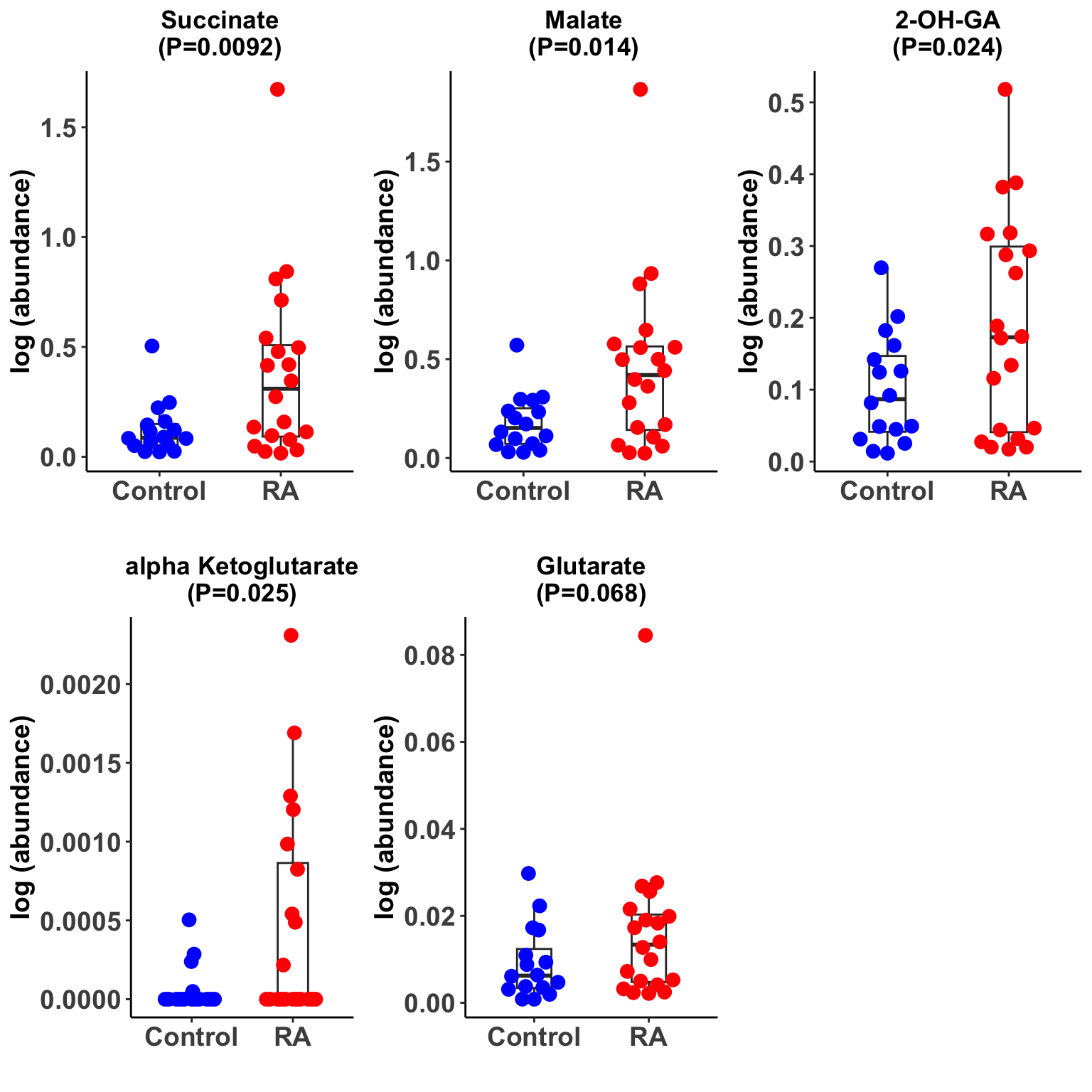

ggsave("../docs/meta_sig_boxplot.pdf", height = 8, width = 8)

Heatmap visualization

All features

library(pheatmap)
#select top 1000 most variant
colAnno <- colData(seMeta)[,"group",drop=FALSE] %>% 
  data.frame()

colAnno$group <- str_replace(colAnno$group, "HC","Control")

seMetaSub <- seMeta[,!is.na(seMeta$dateMeta)]
assay(seMetaSub) <- glog(assay(seMetaSub))
assays(seMetaSub)[["combat"]] <- sva::ComBat(assay(seMetaSub), batch = seMetaSub$dateMeta)

plotMat <- assays(seMetaSub)[["combat"]]

annoColor <- list(group = c(Control = "blue", RA = "red"))

pdf("../docs/meta_heatmap_all.pdf",height = 10, width = 10)
pheatmap(plotMat, scale = "row", 
         annotation_col = colAnno, 
         cluster_rows = T, cluster_cols = FALSE,
         color = colorRampPalette(c("navy", "white", "firebrick"))(100), 
         breaks = seq(-3,3,length.out=100),
         annotation_colors = annoColor, annotation_names_col = FALSE, fontsize_row = 11)
dev.off()

meta_heatmap_all.pdf

Only features with p-value < 0.25

library(pheatmap)
#select top 1000 most variant
#colAnno <- colData(seMeta)[,"group",drop=FALSE] %>% data.frame()

plotMat <- metaMat[filter(resTab, P.Value < 0.25)$metabolite,]

pdf("../docs/meta_heatmap_sig.pdf",height = 4, width = 10)

pheatmap(plotMat, scale = "row", 
         annotation_col = colAnno, 
         cluster_rows = T, cluster_cols = FALSE,
         color = colorRampPalette(c("navy", "white", "firebrick"))(100), 
         breaks = seq(-3,3,length.out=100),
         annotation_colors = annoColor, annotation_names_col = FALSE, fontsize_row = 12)
dev.off()

meta_heatmap_sig.pdf

Write CSV output

write_csv2(select(resTab, metabolite, logFC, P.Value, adj.P.Val), "./metabolite_P_values.csv")
write_csv2(as_tibble(metaMat, rownames = "metabolite"), "./metabolite_normalized_abundance.csv")

Analysis of the proteomic dataset

seProt <- maeObj[["Proteome"]]
dim(seProt)

[1] 2460   12

Heatmap visualization

library(pheatmap)
#select top 1000 most variant
colAnno <- colData(seProt)[,c(1:13,19:22)] %>% data.frame()

protMat <- assays(seProt)[["imputed"]]
sds <- genefilter::rowSds(protMat)
protMat <- protMat[order(sds, decreasing = T)[1:1000],]

pheatmap(protMat, show_rownames = FALSE, scale = "row", 
         annotation_col = colAnno,
         clustering_method = "ward.D2")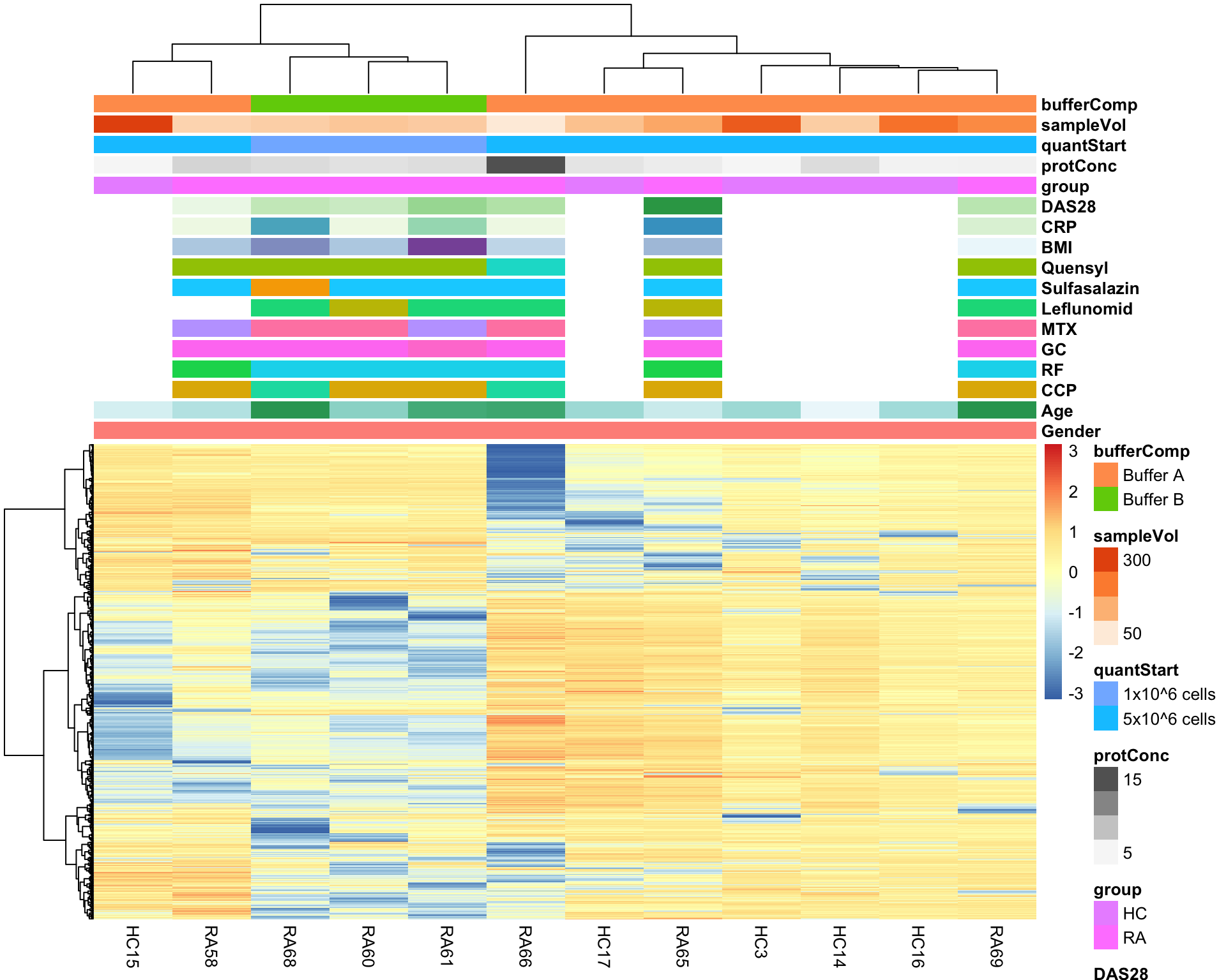

PCA

prRes <- prcomp(t(protMat), scale. = TRUE, center = TRUE)
plotTab <- prRes$x %>% as_tibble(rownames = "sampleID") %>%
    left_join(as_tibble(colAnno, rownames = "sampleID"))

ggplot(plotTab, aes(x=PC1, y=PC2, col = group, shape = bufferComp)) +
    geom_point(size=5) +
    ggrepel::geom_text_repel(aes(label = sampleID))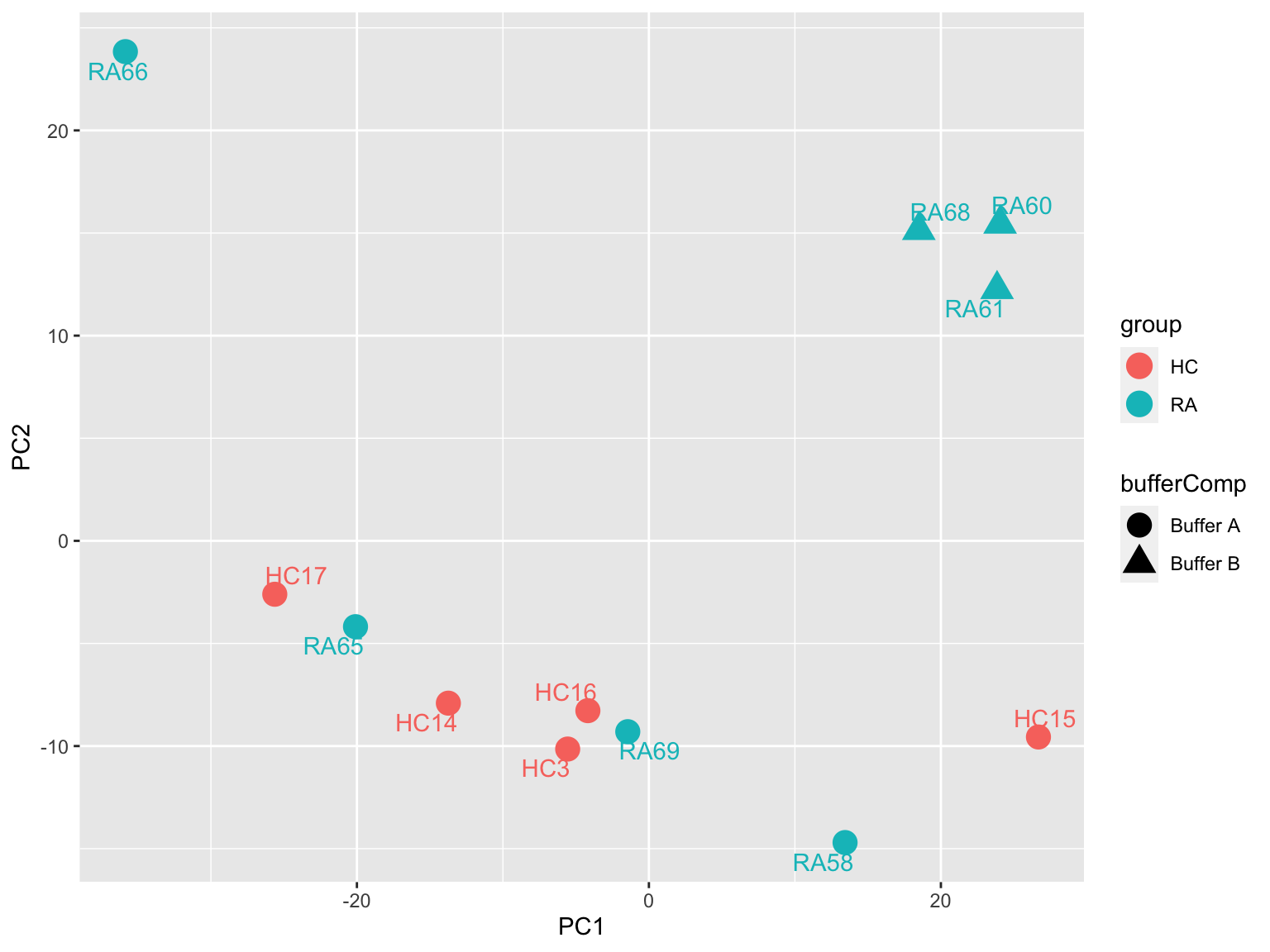

Differential expression using proDA

Differential protein expression using proDA, blocked for buffer condition

library(proDA)
protMat <- assays(seProt)[["norm"]]
designMat <- model.matrix(~ bufferComp + group , colData(seProt))
fit <- proDA(protMat, design = designMat)

resTab <- test_diff(fit, contrast = "groupRA") %>%
  arrange(pval) %>%
  mutate(symbol = rowData(seProt[name,])$symbol)
resTab_prot <- resTab

Warning: The above code chunk cached its results, but it won’t be re-run if previous chunks it depends on are updated. If you need to use caching, it is highly recommended to also set knitr::opts_chunk$set(autodep = TRUE) at the top of the file (in a chunk that is not cached). Alternatively, you can customize the option dependson for each individual chunk that is cached. Using either autodep or dependson will remove this warning. See the knitr cache options for more details.

hist(resTab$pval)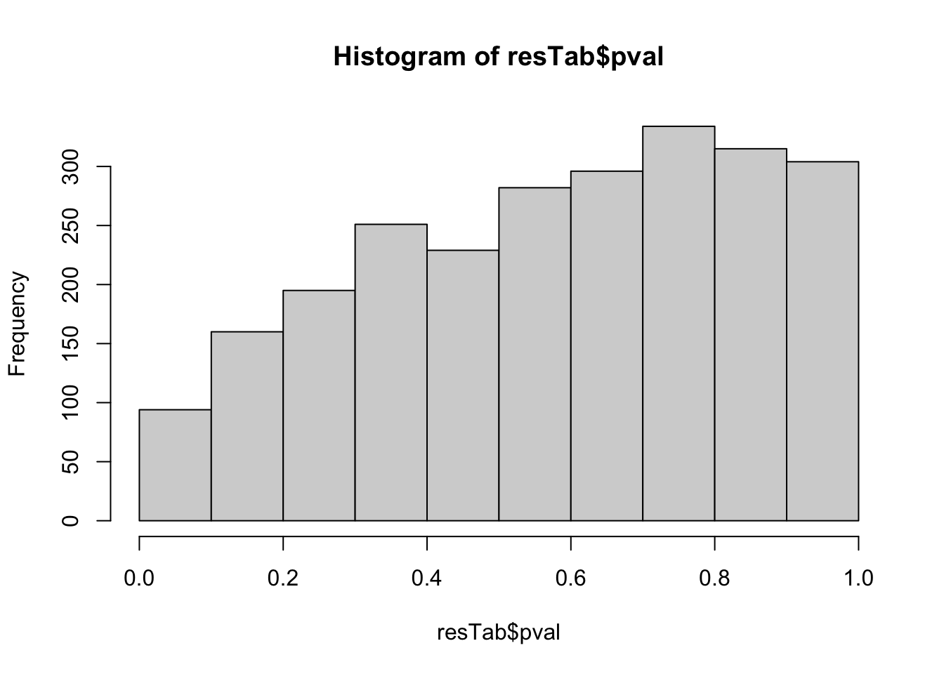

Not strong difference

Proteins with p-value < 0.05

resTab.sig <- filter(resTab, pval < 0.05)
resTab.sig %>% select(symbol, pval, adj_pval, diff) %>%
  mutate_if(is.numeric, formatC, digits=1) %>%
  DT::datatable()

Plot top 9 examples

pList <- lapply(seq(9), function(i) {
  rec <- resTab.sig[i,]
  plotTab <- tibble(expr = protMat[rec$name,],
                    group = seProt$group,
                    bufferComp = seProt$bufferComp) 
  ggplot(plotTab, aes(x=group, y=expr)) +
    geom_boxplot(outlier.shape = NA) +
    ggbeeswarm::geom_quasirandom(aes(color = group, shape = bufferComp), size=3) +
    ggtitle(rec$symbol) +
    theme_bw()
})

cowplot::plot_grid(plotlist = pList,ncol=3)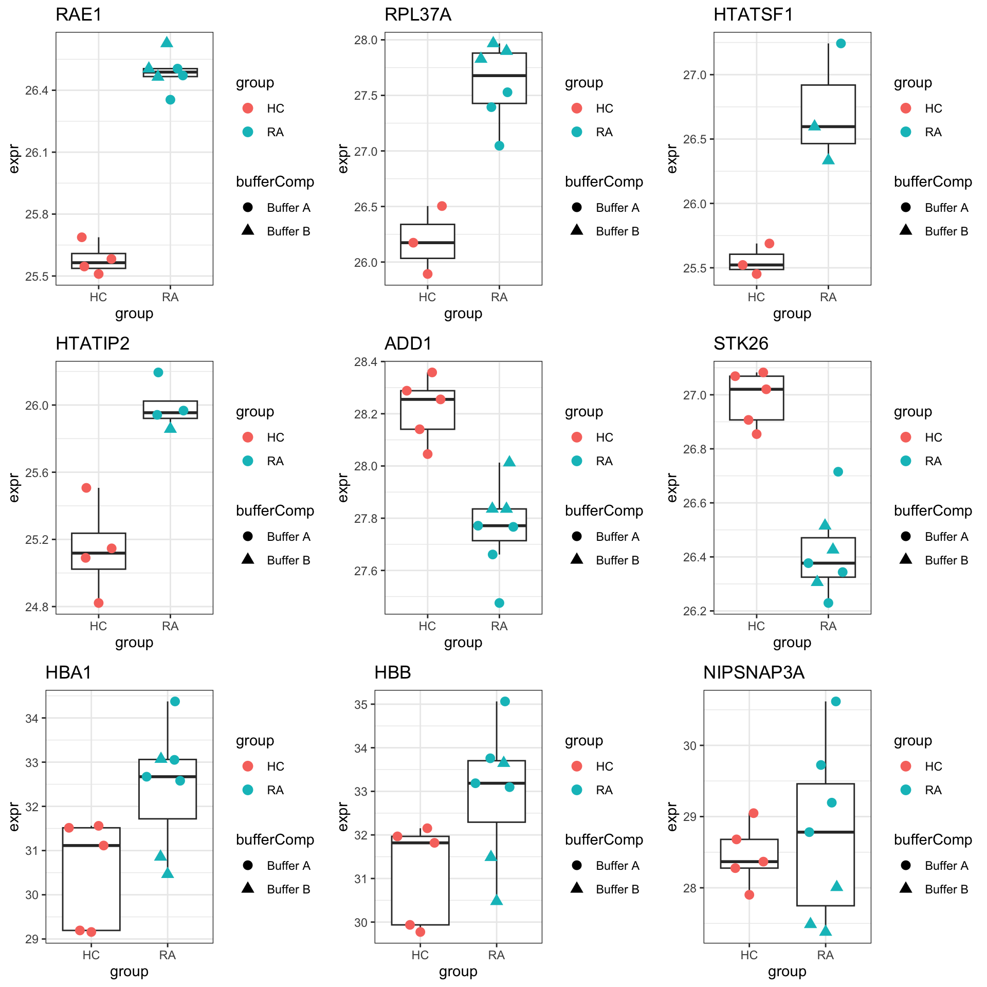

Enrichment analysis

gmts = list(H= "~/EMBL_projects/data/commonFiles/h.all.v6.2.symbols.gmt",
            KEGG = "~/EMBL_projects/data/commonFiles/c2.cp.kegg.v6.2.symbols.gmt",
            C6 = "~/EMBL_projects/data/commonFiles/c6.all.v6.2.symbols.gmt",
            GOBP = "~/EMBL_projects/data/commonFiles/c5.bp.v6.2.symbols.gmt")
inputTab <- resTab %>% filter(pval < 0.1) %>%
  distinct(symbol, .keep_all = TRUE) %>%
  select(symbol, t_statistic) %>% data.frame() %>% column_to_rownames("symbol")
enRes <- list()
enRes[["Hallmark"]] <- runGSEA(inputTab, gmts$H, "page")
enRes[["KEGG"]] <- runGSEA(inputTab, gmts$KEGG,"page")
enRes[["Perturbation"]] <- runGSEA(inputTab, gmts$C6,"page")
enRes[["GOBP"]] <- runGSEA(inputTab, gmts$GOBP,"page")
p <- plotEnrichmentBar(enRes, pCut =0.05, ifFDR= FALSE)
cowplot::plot_grid(p)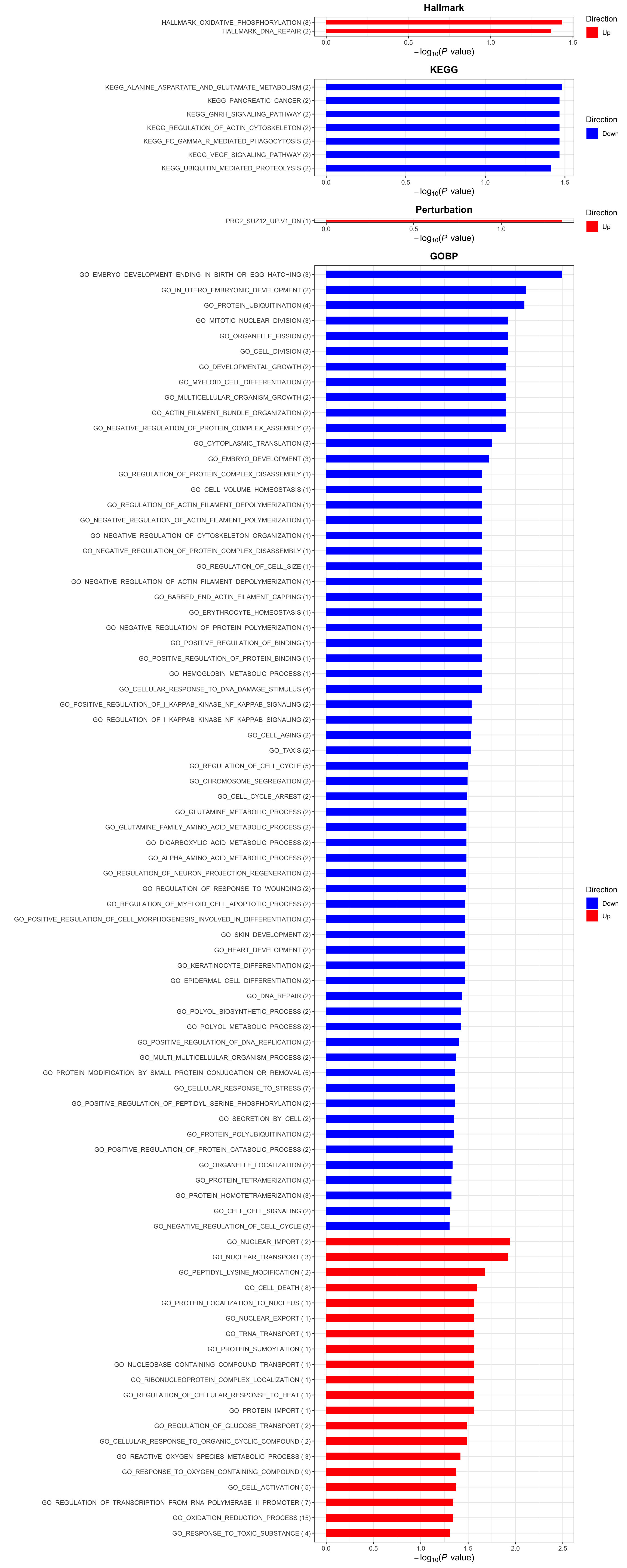

Association between protein expression and enhancer methylation levels

Are there any overlap between differential expressed proteins and differential methylated enhancer CpGs for the same protein?

#get significant protiens
resTab_prot <- resTab_prot %>%
  filter(pval < 0.05) %>%
  dplyr::rename(fc.prot = diff, p.prot = pval, padj.prot = adj_pval, protID = name) %>%
  select(protID, symbol, fc.prot, p.prot, padj.prot)

#get significant enhancer CpGs list
load("../output/resTab_enhancerCpG.RData")
resTab_enhancerCpG <- filter(resTab_enhancerCpG, P.Value < 0.01) %>%
  select(-B, -symbol) %>% dplyr::rename(p.cpg = P.Value, padj.cpg = adj.P.Val, fc.cpg = logFC, fc.cpg.beta = logFC_beta, symbol = gene)

#Get DMR regions
dmrRes <- readxl::read_xlsx("../docs/DMR_GeneHancer.xlsx") %>% filter(p.value < 0.01) %>%
  dplyr::rename(fc.dmr = estimate, p.dmr = p.value, padj.dmr = p.adjust, symbol = gene) %>%
  select(-c(enhancerId, feature, chr, start, end)) %>%
  arrange(p.dmr) %>% distinct(symbol,.keep_all = TRUE)

resTab.com <- resTab_enhancerCpG %>% left_join(resTab_prot, by ="symbol") %>%
  left_join(dmrRes, by = "symbol") %>%
  filter(!is.na(p.prot), !is.na(p.cpg))

Overlapped proteins

unique(sort(resTab.com$symbol))

[1] "FABP5"  "MAP2K1"

Only two proteins

Write CSV output

write_csv2(select(resTab, symbol, diff, pval, adj_pval) %>% dplyr::rename(logFC = diff), "../docs/protein_P_values.csv")
write_csv2(as_tibble(protMat, rownames = "id") %>%
             mutate(symbol = rowData(seProt)[id,]$symbol) %>%
             select(-id), "../docs/protein_normalized_abundance.csv")

P value table

Protein expression table

Analysis of phospho dataset

sePhos <- maeObj[["Phosphoproteome"]]

Heatmap visualization

library(pheatmap)
#select top 1000 most variant
colAnno <- colData(seProt)[,c(1:13,19:22)] %>% data.frame()

protMat <- assays(sePhos)[["imputed"]]
sds <- genefilter::rowSds(protMat)
protMat <- protMat[order(sds, decreasing = T)[1:1000],]

pheatmap(protMat, show_rownames = FALSE, scale = "row", 
         annotation_col = colAnno,
         clustering_method = "ward.D2")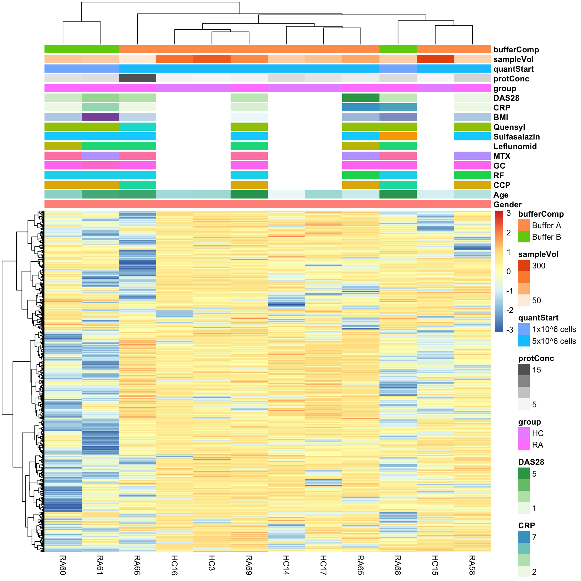

PCA

prRes <- prcomp(t(protMat), scale. = TRUE, center = TRUE)
plotTab <- prRes$x %>% as_tibble(rownames = "sampleID") %>%
    left_join(as_tibble(colAnno, rownames = "sampleID"))

ggplot(plotTab, aes(x=PC1, y=PC2, col = group, shape  = bufferComp)) +
    geom_point(size=5) +
    ggrepel::geom_text_repel(aes(label = sampleID))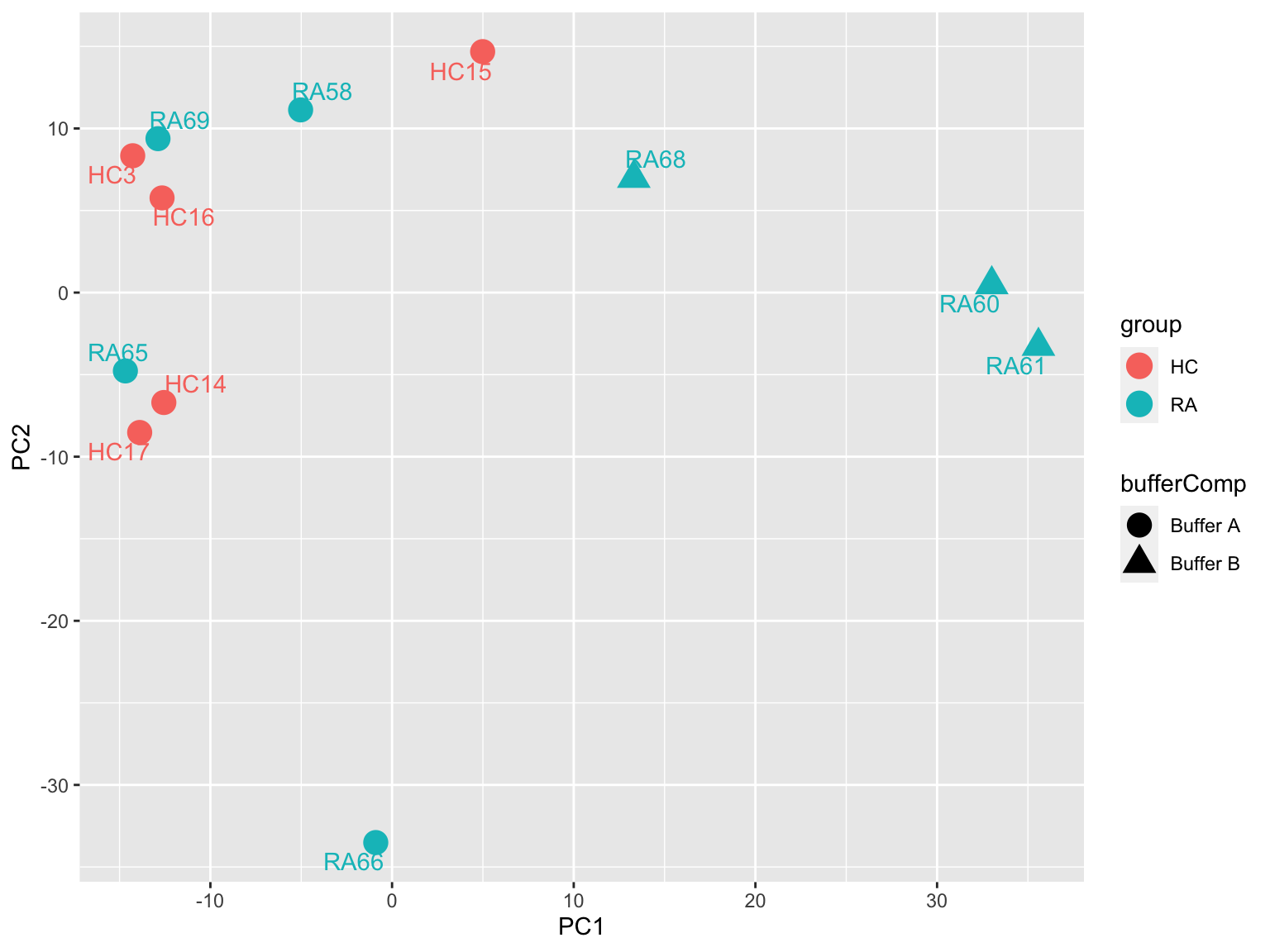

Buffer composition may act as a confounding factor. One sample, RA62 may be outlier.

Differential expression using proDA

Differential protein expression using proDA

protMat <- assays(sePhos)[["norm"]]
designMat <- model.matrix(~ group + bufferComp , colData(sePhos))
fit <- proDA(protMat, design = designMat)

resTab <- test_diff(fit, contrast = "groupRA") %>%
  arrange(pval) %>%
  mutate(symbol = rowData(sePhos)[name,]$symbol,
         site = rowData(sePhos)[name,]$site)

hist(resTab$pval)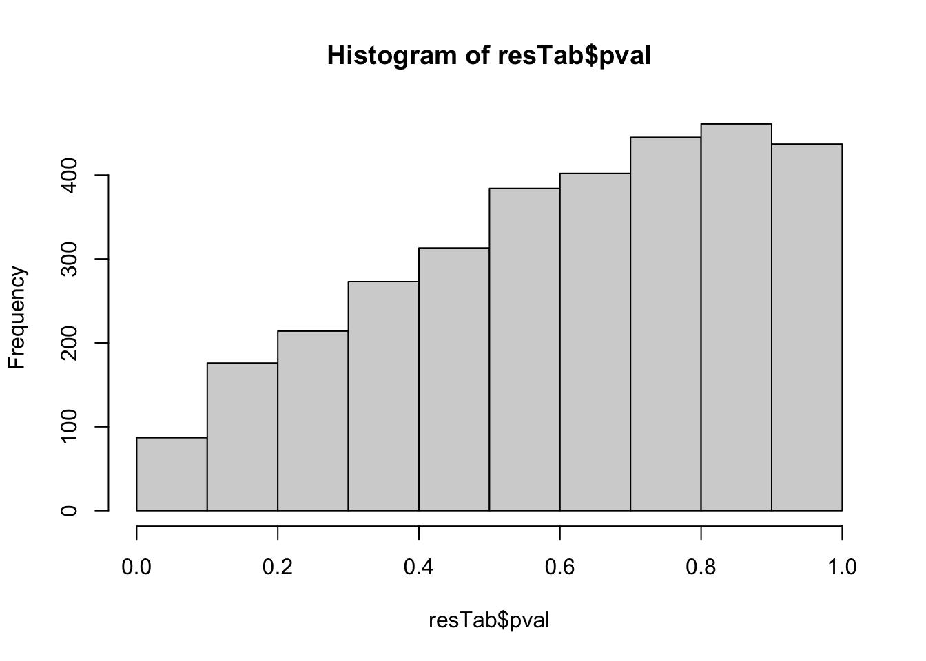

Not strong difference

Proteins with p-value < 0.05

resTab.sig <- filter(resTab, pval < 0.05)
resTab.sig %>% select(symbol, site, pval, adj_pval, diff) %>%
  mutate_if(is.numeric, formatC, digits=1) %>%
  DT::datatable()

Plot top 9 examples

pList <- lapply(seq(9), function(i) {
  rec <- resTab.sig[i,]
  plotTab <- tibble(expr = protMat[rec$name,],
                    group = sePhos$group,
                    bufferComp = sePhos$bufferComp) 
  ggplot(plotTab, aes(x=group, y=expr)) +
    geom_boxplot(outlier.shape = NA) +
    ggbeeswarm::geom_quasirandom(aes(color = group, shape = bufferComp), size=3) +
    ggtitle(rec$site) +
    theme_bw()
})

cowplot::plot_grid(plotlist = pList,ncol=3)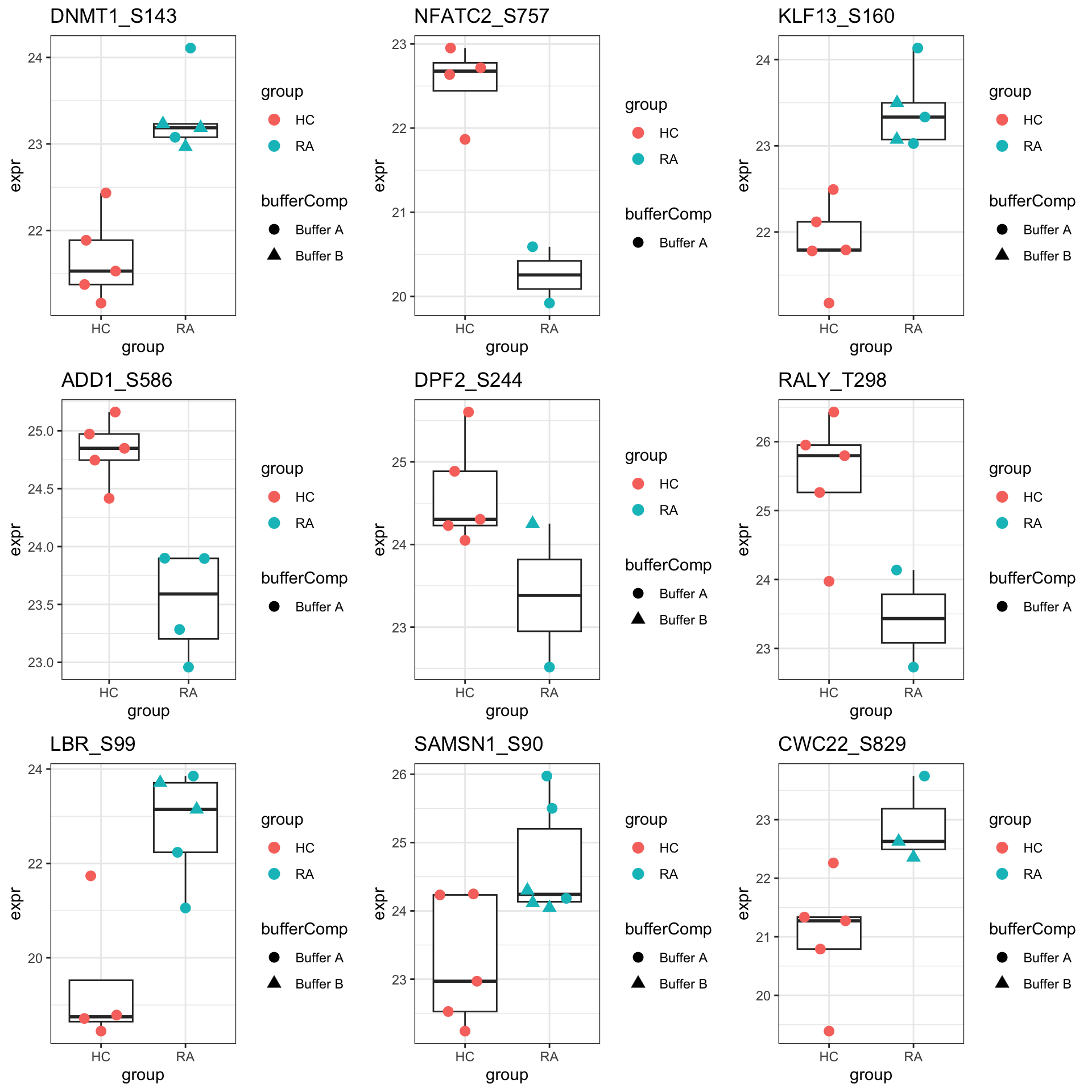

Enrichment analysis

inputTab <- resTab %>% filter(pval < 0.1) %>%
  distinct(symbol, .keep_all = TRUE) %>%
  select(symbol, t_statistic) %>% data.frame() %>% column_to_rownames("symbol")
enRes <- list()
enRes[["Hallmark"]] <- runGSEA(inputTab, gmts$H, "page")
enRes[["KEGG"]] <- runGSEA(inputTab, gmts$KEGG,"page")
enRes[["Perturbation"]] <- runGSEA(inputTab, gmts$C6,"page")
enRes[["GOBP"]] <- runGSEA(inputTab, gmts$GOBP,"page")
p <- plotEnrichmentBar(enRes, pCut =0.05, ifFDR= FALSE)

[1] "No sets passed the criteria"

cowplot::plot_grid(p)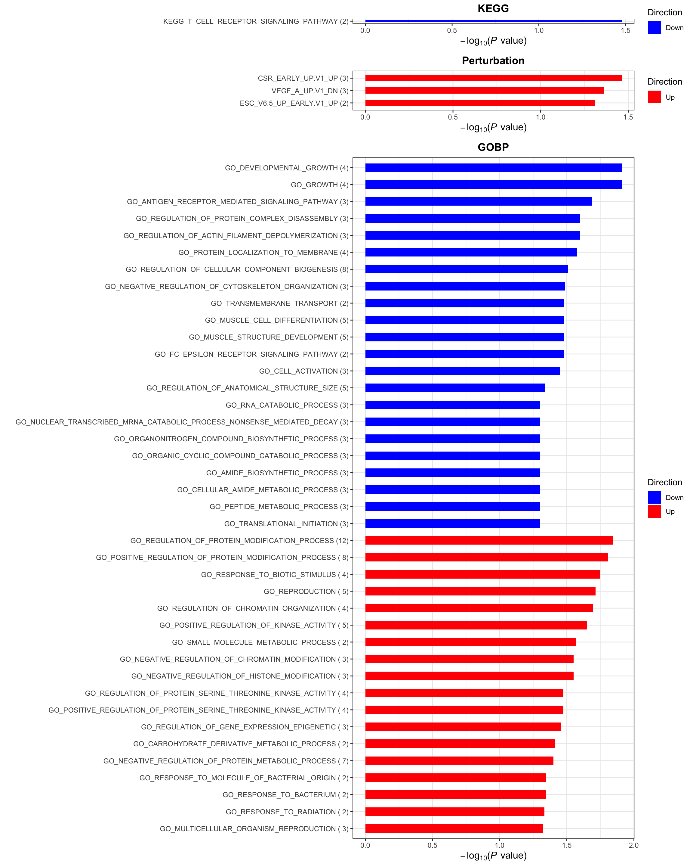

Write CSV output

write_csv2(select(resTab, symbol, site, diff, pval, adj_pval) %>% dplyr::rename(logFC = diff), "../docs/phos_P_values.csv")
write_csv2(as_tibble(protMat, rownames = "id") %>%
             mutate(symbol = rowData(sePhos)[id,]$symbol,
                    site = rowData(sePhos)[id,]$site) %>%
             select(-id), "../docs/phosphorylation_normalized_abundance.csv")

P value table
Phospho abundance table

Kinase activity analysis using decoupler

library(PHONEMeS)
library(decoupleR)

#get decoupler network
decoupler_network <- phonemesPKN %>% 
  dplyr::rename("mor" = interaction) %>% 
  tibble::add_column("likelihood" = 1)

#define decoupler input
decoupler_input <- resTab %>% 
  dplyr::filter(site %in% decoupler_network$target) %>%
  distinct(site, .keep_all = TRUE) %>%
  tibble::column_to_rownames("site") %>% 
  dplyr::select(t_statistic)

#filter deoupler network
decoupler_network <- decoupleR::intersect_regulons(mat = decoupler_input, 
                                                   network = decoupler_network, 
                                                   .source = source, 
                                                   .target = target, 
                                                   minsize = 5)

#remove overlapped regulons
correlated_regulons <- decoupleR::check_corr(decoupler_network) %>% 
  dplyr::filter(correlation >= 0.9)

decoupler_network <- decoupler_network %>% 
  dplyr::filter(!source %in% correlated_regulons$source.2)

# run mlm to estimate kinase activities
kinase_activity <- decoupleR::run_mlm(mat = decoupler_input, 
                                      network = decoupler_network)

head(kinase_activity)

# A tibble: 6 × 5
  statistic source condition     score p_value
  <chr>     <chr>  <chr>         <dbl>   <dbl>
1 mlm       SGK1   t_statistic  1.74    0.0832
2 mlm       CHEK1  t_statistic -0.244   0.807 
3 mlm       AURKA  t_statistic -1.04    0.301 
4 mlm       PDPK1  t_statistic -1.04    0.300 
5 mlm       PRKY   t_statistic -0.0912  0.927 
6 mlm       ROCK2  t_statistic -0.593   0.554

Analysis of phospho dataset (normalized by protein expression)

sePhos <- maeObj[["PhosRatio"]]
sePhos$group <- maeObj[,sePhos$colID]$group
#colData(sePhos) <- colData(maeObj[,colnames(sePhos)])

Differential expression using proDA

Differential protein expression using proDA

protMat <- assays(sePhos)[["ratio"]]
designMat <- model.matrix(~ group + bufferComp, colData(sePhos))
fit <- proDA(protMat, design = designMat)

resTab <- test_diff(fit, contrast = "groupRA") %>%
  arrange(pval) %>%
  mutate(symbol = rowData(sePhos)[name,]$symbol,
         site = rowData(sePhos)[name,]$site)

hist(resTab$pval)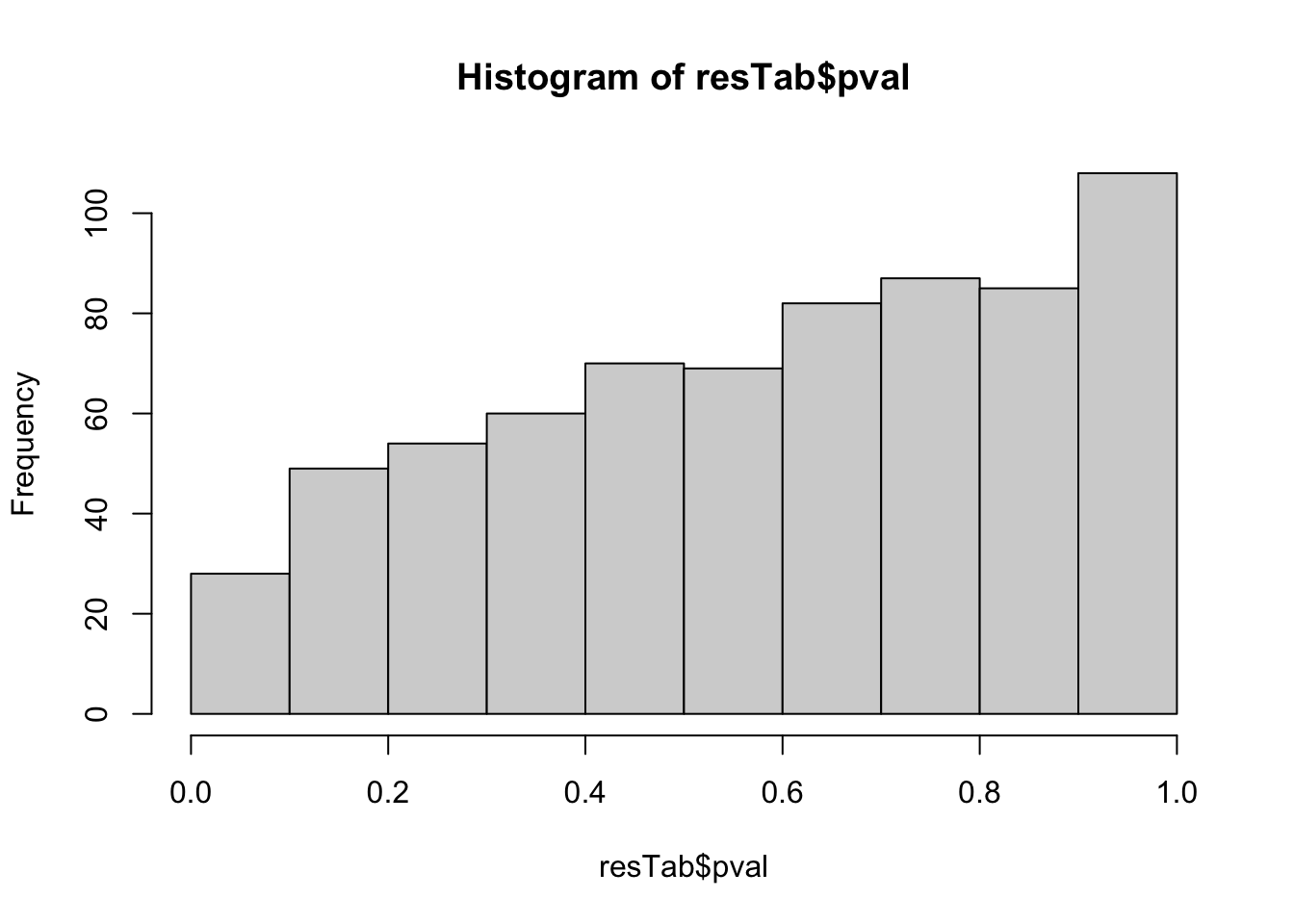

Not strong difference

Proteins with p-value < 0.05

resTab.sig <- filter(resTab, pval < 0.05)
resTab.sig %>% select(symbol, site, pval, adj_pval, diff) %>%
  mutate_if(is.numeric, formatC, digits=1) %>%
  DT::datatable()

Plot top 9 examples

pList <- lapply(seq(9), function(i) {
  rec <- resTab.sig[i,]
  plotTab <- tibble(expr = protMat[rec$name,],
                    group = sePhos$group,
                    bufferComp = sePhos$bufferComp) 
  ggplot(plotTab, aes(x=group, y=expr)) +
    geom_boxplot(outlier.shape = NA) +
    ggbeeswarm::geom_quasirandom(aes(color = group, shape = bufferComp), size=3) +
    ggtitle(rec$site) +
    theme_bw()
})

cowplot::plot_grid(plotlist = pList,ncol=3)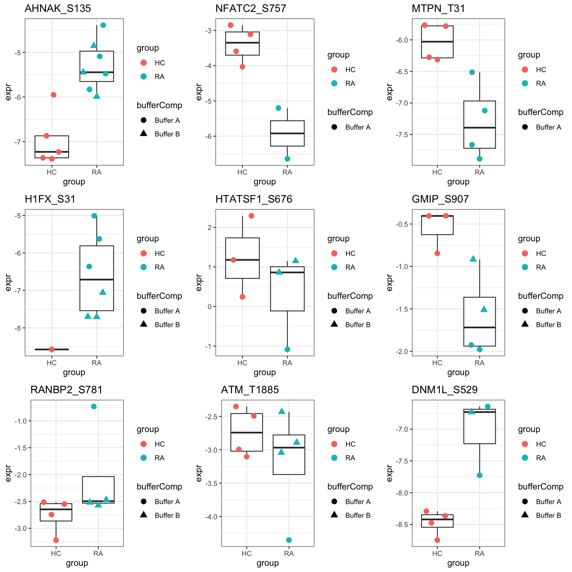

Enrichment analysis

inputTab <- resTab %>% filter(pval < 0.1) %>%
  distinct(symbol, .keep_all = TRUE) %>%
  select(symbol, t_statistic) %>% data.frame() %>% column_to_rownames("symbol")
enRes <- list()
enRes[["Hallmark"]] <- runGSEA(inputTab, gmts$H, "page")
enRes[["KEGG"]] <- runGSEA(inputTab, gmts$KEGG,"page")
enRes[["Perturbation"]] <- runGSEA(inputTab, gmts$C6,"page")
enRes[["GOBP"]] <- runGSEA(inputTab, gmts$GOBP,"page")
p <- plotEnrichmentBar(enRes, pCut =0.05, ifFDR= FALSE)

[1] "No sets passed the criteria"

cowplot::plot_grid(p)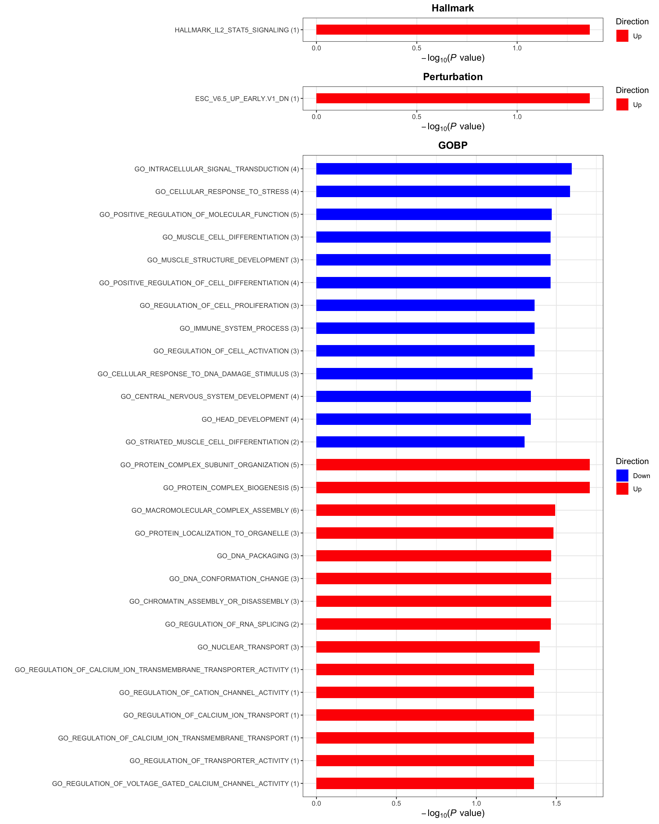

Write CSV output

write_csv2(select(resTab, symbol, site, diff, pval, adj_pval) %>% dplyr::rename(logFC = diff), "../docs/phos_P_values_protNorm.csv")
write_csv2(as_tibble(protMat, rownames = "id") %>%
             mutate(symbol = rowData(sePhos)[id,]$symbol,
                    site = rowData(sePhos)[id,]$site) %>%
             select(-id), "../docs/phosphorylation_ProtNormalized_abundance.csv")

P value table
Phospho abundance table

Kinase activity analysis using decoupler

#get decoupler network
decoupler_network <- phonemesPKN %>% 
  dplyr::rename("mor" = interaction) %>% 
  tibble::add_column("likelihood" = 1)

#define decoupler input
decoupler_input <- resTab %>% 
  dplyr::filter(site %in% decoupler_network$target) %>%
  distinct(site, .keep_all = TRUE) %>%
  tibble::column_to_rownames("site") %>% 
  dplyr::select(t_statistic)

#filter deoupler network
decoupler_network <- decoupleR::intersect_regulons(mat = decoupler_input, 
                                                   network = decoupler_network, 
                                                   .source = source, 
                                                   .target = target, 
                                                   minsize = 5)

#remove overlapped regulons
correlated_regulons <- decoupleR::check_corr(decoupler_network) %>% 
  dplyr::filter(correlation >= 0.9)

decoupler_network <- decoupler_network %>% 
  dplyr::filter(!source %in% correlated_regulons$source.2)

# run mlm to estimate kinase activities
kinase_activity <- decoupleR::run_mlm(mat = decoupler_input, 
                                      network = decoupler_network)

head(kinase_activity)

# A tibble: 6 × 5
  statistic source condition    score p_value
  <chr>     <chr>  <chr>        <dbl>   <dbl>
1 mlm       PRKY   t_statistic  0.145   0.885
2 mlm       PRKCG  t_statistic -0.464   0.643
3 mlm       PRKCB  t_statistic  0.198   0.843
4 mlm       CDK1   t_statistic  0.384   0.701
5 mlm       PRKCA  t_statistic  0.108   0.914
6 mlm       PRKACA t_statistic -0.120   0.905

FACS data

seFacs <- maeObj[["FACS"]]
facsTab <- sumToTidy(seFacs, rowID = "id", colID = "sampleID")
facsMat <- assay(seFacs)

Vsn

facsMat.vst <- vsn::justvsn(facsMat)
#meanSdPlot(facsMat.vst)

PCA

Perform PCA

pcMat <- facsMat.vst
pcMat <- pcMat[complete.cases(pcMat),]
pcRes <- prcomp(t(pcMat), scale. = TRUE, center = TRUE)$x
plotTab <- as_tibble(pcRes, rownames = "colID") %>%
    left_join(as.tibble(colData(seFacs), rownames = "colID"))
   
ggplot(plotTab, aes(x=PC1, y=PC2, col = group, label = sampleID)) +
    geom_point() +
    ggrepel::geom_text_repel()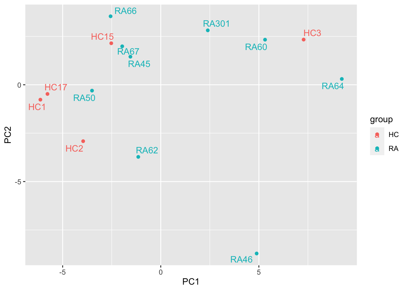

Differential test

designMat <- model.matrix(~group, data = colData(seFacs))
lmFit <- lmFit(facsMat.vst, design = designMat)
fit2 <- eBayes(lmFit)
resTab <- topTable(fit2, number = Inf) %>%
    as_tibble(rownames = "id") %>%
    mutate(feature = rowData(seFacs[id,])$feature)
hist(resTab$P.Value)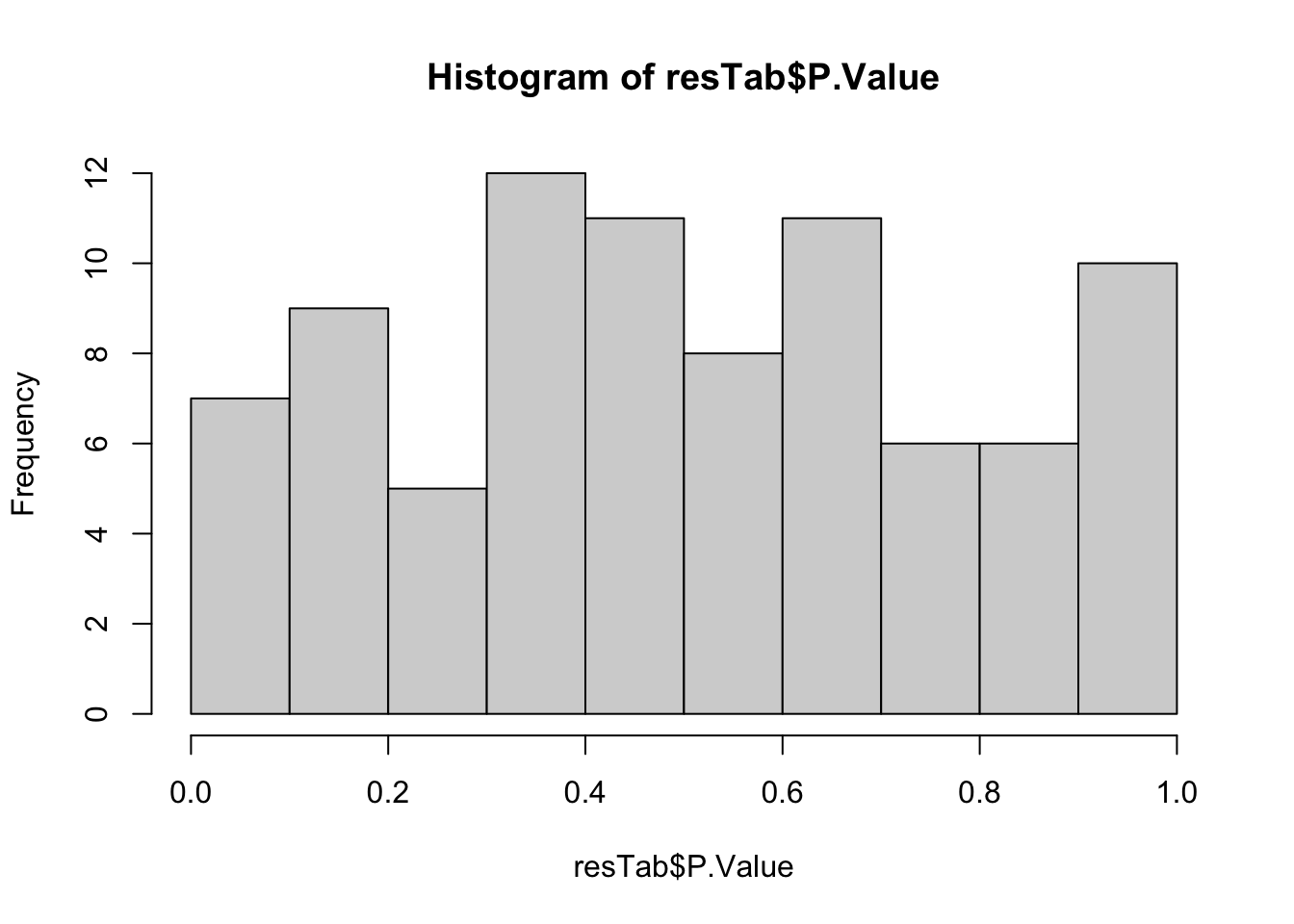

head(resTab)

# A tibble: 6 × 8
  id     logFC AveExpr     t P.Value adj.P.Val     B feature              
  <chr>  <dbl>   <dbl> <dbl>   <dbl>     <dbl> <dbl> <chr>                
1 f36    0.910    9.49  2.30  0.0351     0.910 -4.51 effector memory PD1  
2 f29   -0.910    5.07 -2.18  0.0444     0.910 -4.52 effector memory CTLA4
3 f49   -0.634    5.42 -2.06  0.0556     0.910 -4.53 effector TEMRA CTLA4 
4 f56    0.945    9.08  2.02  0.0604     0.910 -4.53 effector TEMRA PD1   
5 f74   -0.826   13.1  -1.91  0.0746     0.910 -4.54 naive LDHA           
6 f17   -0.932   13.3  -1.86  0.0807     0.910 -4.54 central memory LDHA

Plot significant associations

pList <- lapply(seq(nrow(filter(resTab, P.Value <= 0.05))), function(i) {
    rec <- resTab[i,]
    plotTab <- filter(facsTab, id == rec$id)
    ggplot(plotTab, aes(x=group, y=count, label = sampleID)) + 
        geom_boxplot(outlier.shape = NA) + 
        ggbeeswarm::geom_quasirandom(aes(color = group), size=3) +
        ggtitle(sprintf("%s (P=%s)",rec$feature,formatC(rec$P.Value,digits = 2))) +
        ggrepel::geom_text_repel() +
        theme_bw() +
        theme(legend.position = "none")
})
cowplot::plot_grid(plotlist = pList,ncol=3)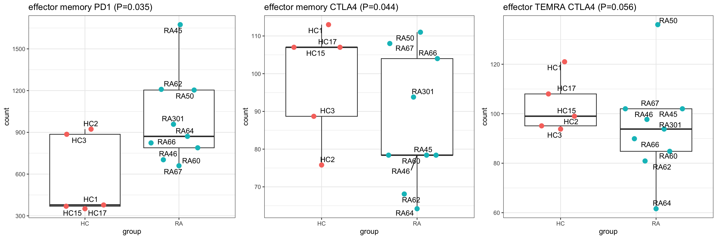

sessionInfo()

R version 4.2.0 (2022-04-22)
Platform: x86_64-apple-darwin17.0 (64-bit)
Running under: macOS Big Sur/Monterey 10.16

Matrix products: default
BLAS:   /Library/Frameworks/R.framework/Versions/4.2/Resources/lib/libRblas.0.dylib
LAPACK: /Library/Frameworks/R.framework/Versions/4.2/Resources/lib/libRlapack.dylib

locale:
[1] en_US.UTF-8/en_US.UTF-8/en_US.UTF-8/C/en_US.UTF-8/en_US.UTF-8

attached base packages:
[1] stats4    stats     graphics  grDevices utils     datasets  methods  
[8] base     

other attached packages:
 [1] decoupleR_2.2.2             PHONEMeS_2.0.1             
 [3] piano_2.12.0                pheatmap_1.0.12            
 [5] limma_3.52.2                forcats_0.5.1              
 [7] stringr_1.4.1               dplyr_1.1.4.9000           
 [9] purrr_0.3.4                 readr_2.1.2                
[11] tidyr_1.2.0                 tibble_3.2.1               
[13] ggplot2_3.4.1               tidyverse_1.3.2            
[15] proDA_1.10.0                MultiAssayExperiment_1.22.0
[17] SummarizedExperiment_1.26.1 Biobase_2.56.0             
[19] GenomicRanges_1.48.0        GenomeInfoDb_1.32.2        
[21] IRanges_2.30.0              S4Vectors_0.34.0           
[23] BiocGenerics_0.42.0         MatrixGenerics_1.8.1       
[25] matrixStats_0.62.0          jyluMisc_0.1.5             

loaded via a namespace (and not attached):
  [1] utf8_1.2.4             shinydashboard_0.7.2   tidyselect_1.2.1      
  [4] RSQLite_2.2.15         AnnotationDbi_1.58.0   htmlwidgets_1.5.4     
  [7] grid_4.2.0             BiocParallel_1.30.4    maxstat_0.7-25        
 [10] munsell_0.5.0          preprocessCore_1.58.0  ragg_1.2.2            
 [13] codetools_0.2-18       DT_0.23                withr_3.0.0           
 [16] colorspace_2.0-3       highr_0.9              knitr_1.39            
 [19] rstudioapi_0.13        ggsignif_0.6.3         labeling_0.4.2        
 [22] git2r_0.30.1           slam_0.1-50            GenomeInfoDbData_1.2.8
 [25] KMsurv_0.1-5           bit64_4.0.5            farver_2.1.1          
 [28] rprojroot_2.0.3        vctrs_0.6.5            generics_0.1.3        
 [31] TH.data_1.1-1          xfun_0.31              sets_1.0-21           
 [34] R6_2.5.1               ggbeeswarm_0.6.0       locfit_1.5-9.6        
 [37] bitops_1.0-7           cachem_1.0.6           fgsea_1.22.0          
 [40] DelayedArray_0.22.0    assertthat_0.2.1       vroom_1.5.7           
 [43] promises_1.2.0.1       scales_1.2.0           multcomp_1.4-26       
 [46] googlesheets4_1.0.0    beeswarm_0.4.0         gtable_0.3.0          
 [49] extraDistr_1.9.1       affy_1.74.0            sva_3.44.0            
 [52] sandwich_3.0-2         workflowr_1.7.0        rlang_1.1.3           
 [55] genefilter_1.78.0      systemfonts_1.0.4      splines_4.2.0         
 [58] rstatix_0.7.0          gargle_1.2.0           broom_1.0.0           
 [61] BiocManager_1.30.18    yaml_2.3.5             abind_1.4-5           
 [64] modelr_0.1.8           crosstalk_1.2.0        backports_1.4.1       
 [67] httpuv_1.6.6           tools_4.2.0            relations_0.6-12      
 [70] affyio_1.66.0          ellipsis_0.3.2         gplots_3.1.3          
 [73] RColorBrewer_1.1-3     jquerylib_0.1.4        Rcpp_1.0.11           
 [76] visNetwork_2.1.0       zlibbioc_1.42.0        RCurl_1.98-1.7        
 [79] ggpubr_0.4.0           cowplot_1.1.1          zoo_1.8-10            
 [82] ggrepel_0.9.1          haven_2.5.0            cluster_2.1.3         
 [85] exactRankTests_0.8-35  fs_1.5.2               magrittr_2.0.3        
 [88] data.table_1.14.10     reprex_2.0.1           survminer_0.4.9       
 [91] googledrive_2.0.0      mvtnorm_1.1-3          hms_1.1.1             
 [94] shinyjs_2.1.0          mime_0.12              evaluate_0.15         
 [97] xtable_1.8-4           XML_3.99-0.10          readxl_1.4.0          
[100] gridExtra_2.3          compiler_4.2.0         KernSmooth_2.23-20    
[103] crayon_1.5.2           htmltools_0.5.4        mgcv_1.8-40           
[106] later_1.3.0            tzdb_0.3.0             lubridate_1.8.0       
[109] DBI_1.1.3              dbplyr_2.2.1           MASS_7.3-58           
[112] Matrix_1.5-4           car_3.1-0              cli_3.6.2             
[115] vsn_3.64.0             marray_1.74.0          parallel_4.2.0        
[118] igraph_1.3.4           pkgconfig_2.0.3        km.ci_0.5-6           
[121] xml2_1.3.3             annotate_1.74.0        vipor_0.4.5           
[124] bslib_0.4.1            XVector_0.36.0         drc_3.0-1             
[127] rvest_1.0.2            digest_0.6.30          Biostrings_2.64.0     
[130] rmarkdown_2.14         cellranger_1.1.0       fastmatch_1.1-3       
[133] survMisc_0.5.6         edgeR_3.38.1           shiny_1.7.4           
[136] gtools_3.9.3           lifecycle_1.0.4        nlme_3.1-158          
[139] jsonlite_1.8.3         carData_3.0-5          fansi_1.0.6           
[142] pillar_1.9.0           lattice_0.20-45        KEGGREST_1.36.3       
[145] fastmap_1.1.0          httr_1.4.3             plotrix_3.8-2         
[148] survival_3.4-0         glue_1.7.0             png_0.1-7             
[151] bit_4.0.4              stringi_1.7.8          sass_0.4.2            
[154] blob_1.2.3             textshaping_0.3.6      caTools_1.18.2        
[157] memoise_2.0.1

Explore and analyze each individual single omic dataset

Junyan Lu

Load libraries

Load processed data

Analysis of metabolomic data

Visualize overall data distribution

Per sample

Per metabolite

PCA

Differential abundance test

Heatmap visualization

All features

Only features with p-value < 0.25

Write CSV output

Analysis of the proteomic dataset

Heatmap visualization

PCA

Differential expression using proDA

Proteins with p-value < 0.05

Plot top 9 examples

Enrichment analysis

Association between protein expression and enhancer methylation levels

Are there any overlap between differential expressed proteins and differential methylated enhancer CpGs for the same protein?

Overlapped proteins

Write CSV output

Analysis of phospho dataset

Heatmap visualization

PCA

Differential expression using proDA

Proteins with p-value < 0.05

Plot top 9 examples

Enrichment analysis

Write CSV output

Kinase activity analysis using decoupler

Analysis of phospho dataset (normalized by protein expression)

Differential expression using proDA

Proteins with p-value < 0.05

Plot top 9 examples

Enrichment analysis

Write CSV output

Kinase activity analysis using decoupler

FACS data

Vsn

PCA

Differential test