Exploratory analysis the AML CART-T drug screen project
Junyan Lu
Last updated: 2023-06-06
Checks: 5 1
Knit directory: combiCART/analysis/
This reproducible R Markdown analysis was created with workflowr (version 1.7.0). The Checks tab describes the reproducibility checks that were applied when the results were created. The Past versions tab lists the development history.
Great job! The global environment was empty. Objects defined in the global environment can affect the analysis in your R Markdown file in unknown ways. For reproduciblity it’s best to always run the code in an empty environment.
The command set.seed(20221110) was run prior to running
the code in the R Markdown file. Setting a seed ensures that any results
that rely on randomness, e.g. subsampling or permutations, are
reproducible.
Great job! Recording the operating system, R version, and package versions is critical for reproducibility.
Nice! There were no cached chunks for this analysis, so you can be confident that you successfully produced the results during this run.
Great job! Using relative paths to the files within your workflowr project makes it easier to run your code on other machines.
Tracking code development and connecting the code version to the
results is critical for reproducibility. To start using Git, open the
Terminal and type git init in your project directory.
This project is not being versioned with Git. To obtain the full
reproducibility benefits of using workflowr, please see
?wflow_start.
Load packages and dataset
library(readxl)
library(tidyverse)
knitr::opts_chunk$set(warning = FALSE, message = FALSE)
source("../code/helper.R")
load("../output/screenData.RData")
Compare the effect of Control, CAR-T only and NT only treatment on viability
plotTab <- filter(screenData, Drug == "DMSO")
ggplot(plotTab, aes(x=donorConstruct, y=normVal,dodge = Tcell)) +
  geom_boxplot(position = position_dodge(width = 0.8)) +
  geom_point(aes(col=Tcell), position = position_dodge(width = 0.8)) +
  facet_wrap(~cellTime, scale = "free",ncol=2) +
  theme(axis.text.x = element_text(angle = 90, hjust = 1, vjust = 0.5)) +
  ylab("Viability")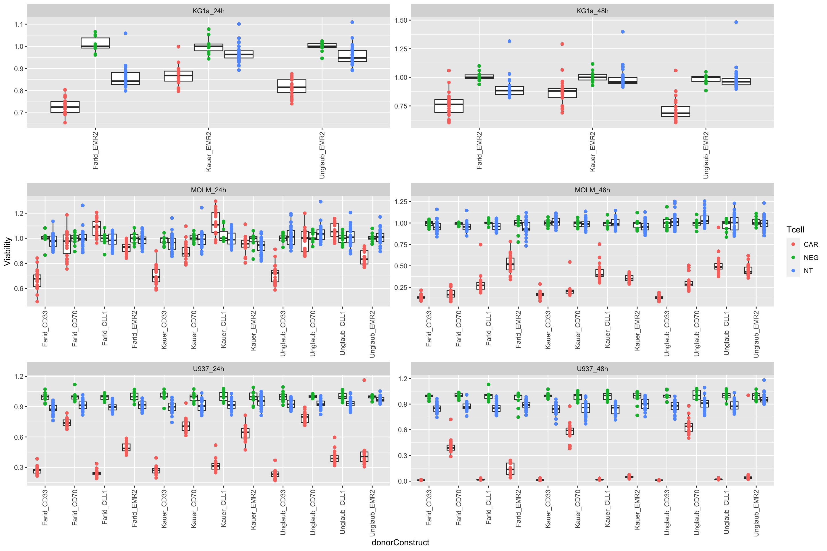
Visualize difference among T cell donors
Compare the trend of cell line with different donors
**Do cells cultured with T-cells from different donors show consistent changes?
donorTab <- filter(screenData, Drug == "DMSO", Tcell != "NEG") %>%
  mutate(cellTimeConst = paste0(cellTime,"_",construct)) %>%
  group_by(Tcell, cellTimeConst, donor) %>%
  summarise(medVal = median(normVal))
ggplot(donorTab, aes(x=cellTimeConst, y=medVal, color = donor)) +
  geom_point() +
  geom_line(aes(group = donor)) +
  facet_wrap(~Tcell, ncol=1) + theme(axis.text.x = element_text(angle = 90, hjust = 1, vjust = 0.5)) +
  ylab("Median viability") + xlab("Cell")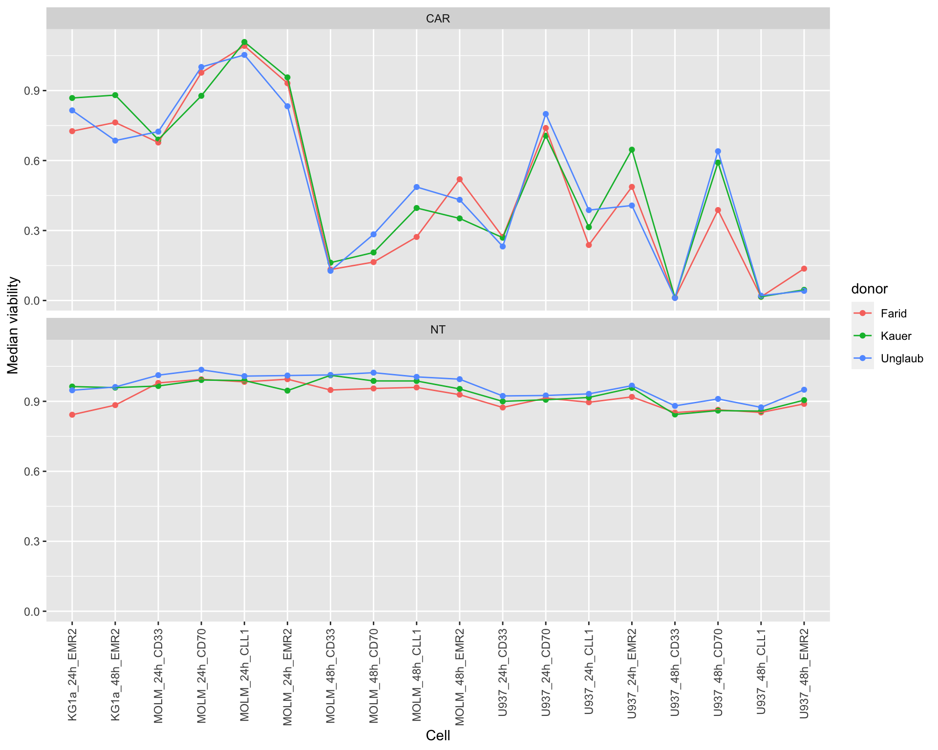
PCA
**Do cells cultured with T-cells from different donors show consistent changes?
viabMat <- filter(screenData, Tcell!="NEG", Drug != "DMSO") %>%
mutate(nameConc = paste0(name,"_",conc)) %>%
group_by(nameConc, plateID) %>% summarise(val = mean(normVal)) %>%
pivot_wider(names_from = nameConc, values_from = val) %>%
column_to_rownames("plateID") %>% as.matrix()
pcTab <- prcomp(viabMat)$x %>%
as_tibble(rownames= "plateID") %>%
left_join(distinct(screenData, plateID, donor, cell, time, construct)) %>%
mutate(celLTimeConst = paste0(cell,time,construct))
ggplot(pcTab, aes(x=PC1, y=PC2)) +
geom_point(aes(col = cell, shape = construct, size = time)) +
geom_line(aes(group = celLTimeConst), linetype = "dashed")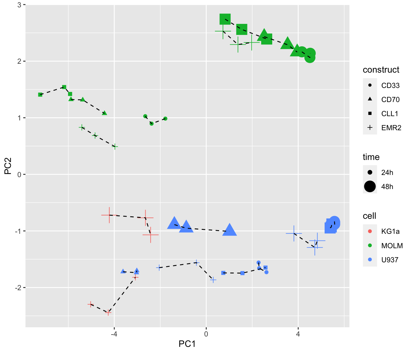 Dotted lines connect the cell models (cellline + time +
construct) with the same T-cell donor. It can be seen that the cell
models with the same donors are loosely grouped together. Indicating
there’s some similarity in their response profile
Dotted lines connect the cell models (cellline + time +
construct) with the same T-cell donor. It can be seen that the cell
models with the same donors are loosely grouped together. Indicating
there’s some similarity in their response profile
Visualize Drug effect
Normalized by tumor only wells
Dose-response curves
plotTab <- filter(screenData, Drug != "DMSO", Tcell == "NT")

pList <- lapply(unique(sort(plotTab$cellTime)),function(nn) {
  eachTab <- filter(plotTab, cellTime == nn)
  ggplot(eachTab, aes(x=conc, y=normVal)) +
    geom_point() +
    geom_line(aes(group = donorConstruct, color = donorConstruct)) +
    facet_wrap(~Drug, scale = "free_x", ncol=4) +
    scale_x_log10() +
    xlab("Concentration") + ylab("Viability") +
    ggtitle(nn)
})

jyluMisc::makepdf(pList, "../docs/drugNT_doseResponse.pdf", ncol=1, nrow=1, height = 15, width = 10)Heatmap of the summarised AUC of drug effect
aucTab <- filter(screenData, Drug != "DMSO", Tcell == "NT") %>%
  group_by(cell, time, donor, construct, Drug, plateID) %>%
  summarise(auc = calcAUC(normVal, conc)) %>% ungroup()

colAnno <- distinct(aucTab, plateID, cell, time, donor, construct) %>%
  column_to_rownames("plateID") %>% data.frame()

viabMat <- aucTab %>% select(plateID, auc, Drug) %>%
  pivot_wider(names_from = plateID, values_from = auc) %>%
  column_to_rownames("Drug") %>% as.matrix()
Without row normalization, colores indicate viability
pheatmap::pheatmap(viabMat, annotation_col = colAnno, show_colnames = TRUE, clustering_method = "ward.D2")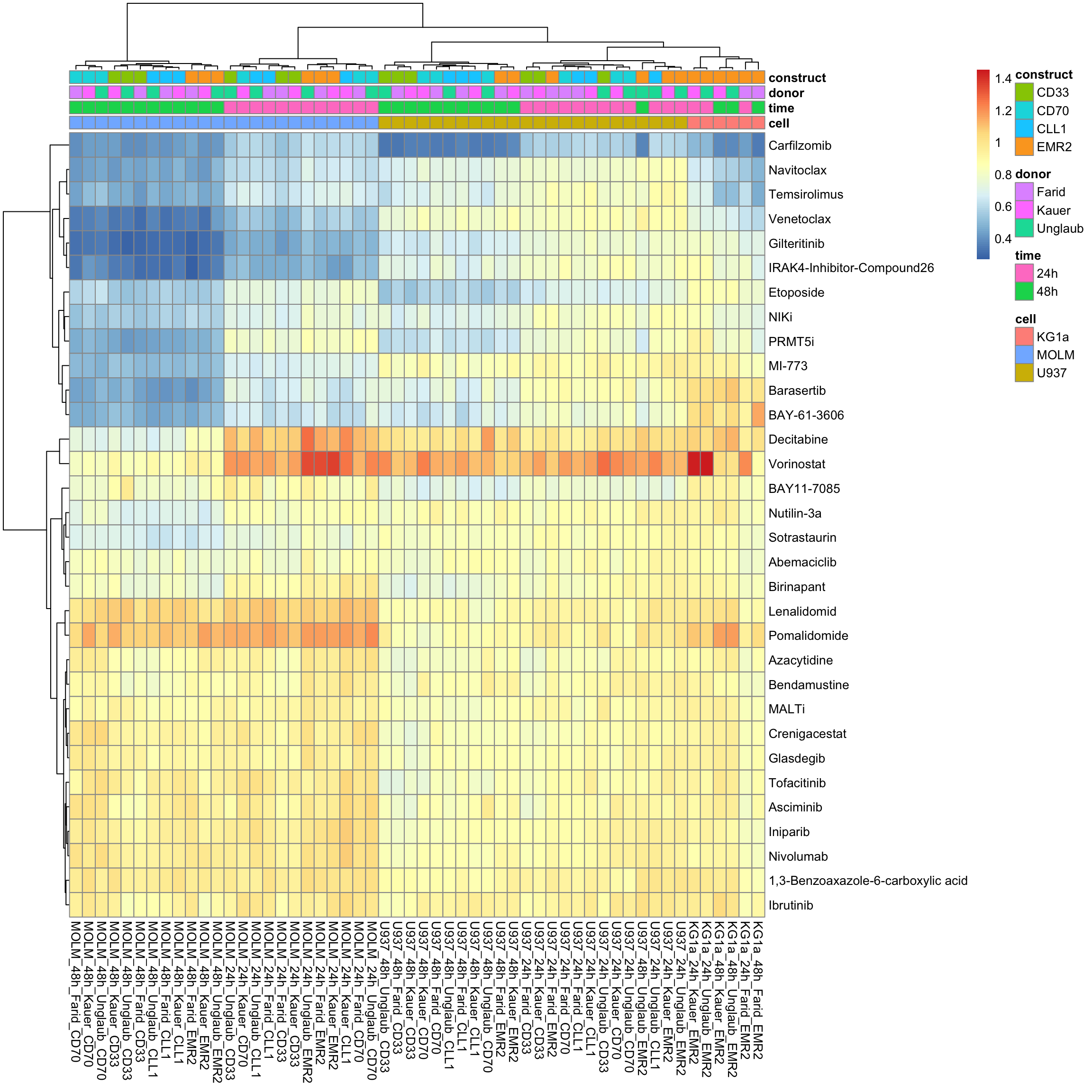
With row normalization, colores indicate row-wise z-scores
pheatmap::pheatmap(viabMat, annotation_col = colAnno, show_colnames = TRUE, clustering_method = "ward.D2", scale = "row")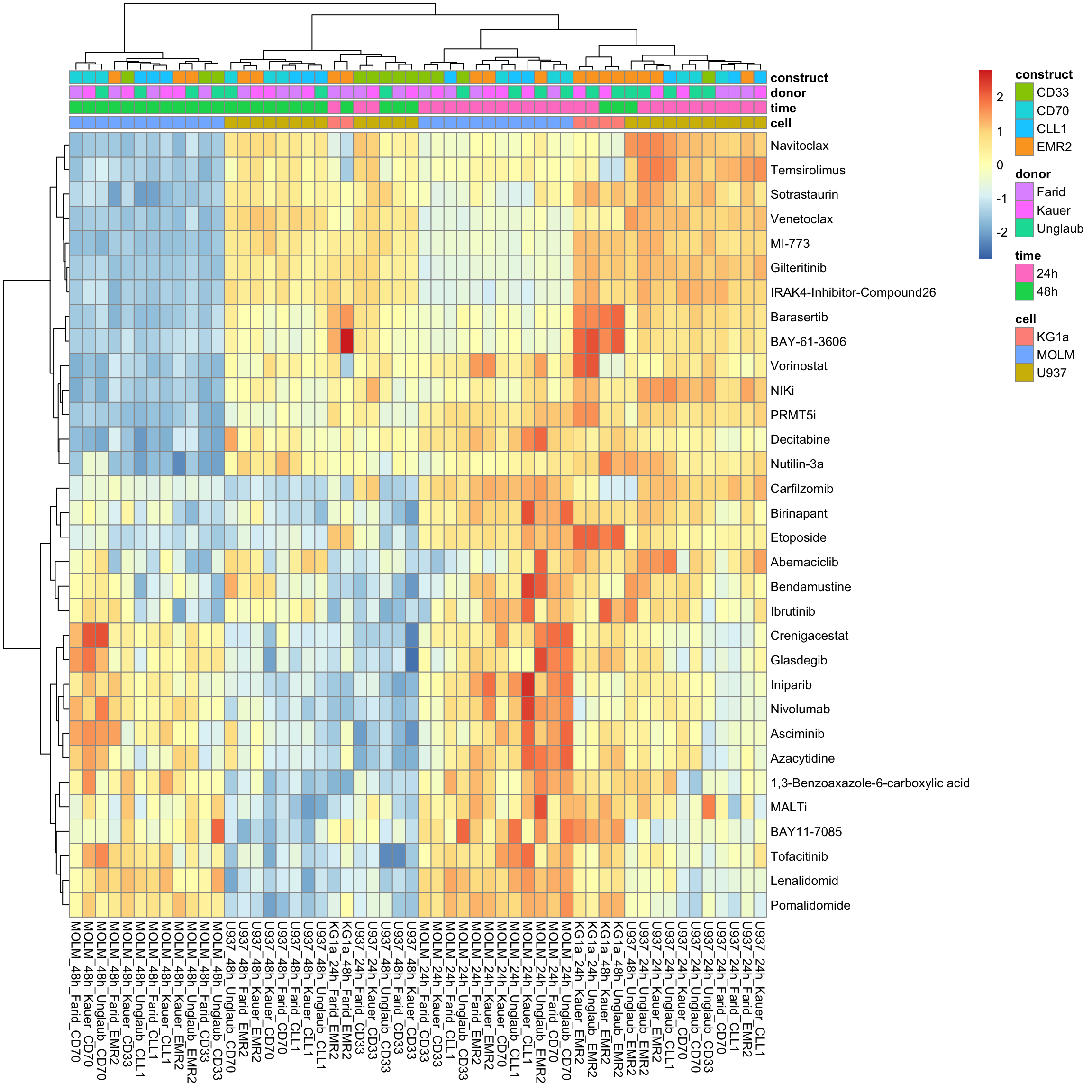
Normalized by NT only wells
Dose-response curves
plotTab <- filter(screenData, Drug != "DMSO", Tcell == "NT")

pList <- lapply(unique(sort(plotTab$cellTime)),function(nn) {
  eachTab <- filter(plotTab, cellTime == nn)
  ggplot(eachTab, aes(x=conc, y=normVal.NT)) +
    geom_point() +
    geom_line(aes(group = donorConstruct, color = donorConstruct)) +
    facet_wrap(~Drug, scale = "free_x", ncol=4) +
    scale_x_log10() +
    xlab("Concentration") + ylab("Viability") +
    ggtitle(nn)
})

jyluMisc::makepdf(pList, "../docs/drugNT_doseResponse_NTnorm.pdf", ncol=1, nrow=1, height = 15, width = 10)
drugNT_doseResponse_NTnorm.pdf
It seems normalization by NT only wells decreased variation among samples.
Heatmap of the summarised AUC of drug effect
aucTab <- filter(screenData, Drug != "DMSO", Tcell == "NT") %>%
  group_by(cell, time, donor, construct, Drug, plateID) %>%
  summarise(auc = calcAUC(normVal.NT, conc)) %>% ungroup()

colAnno <- distinct(aucTab, plateID, cell, time, donor, construct) %>%
  column_to_rownames("plateID") %>% data.frame()

viabMat <- aucTab %>% select(plateID, auc, Drug) %>%
  pivot_wider(names_from = plateID, values_from = auc) %>%
  column_to_rownames("Drug") %>% as.matrix()
Without row normalization, colores indicate viability
pheatmap::pheatmap(viabMat, annotation_col = colAnno, show_colnames = TRUE, clustering_method = "ward.D2")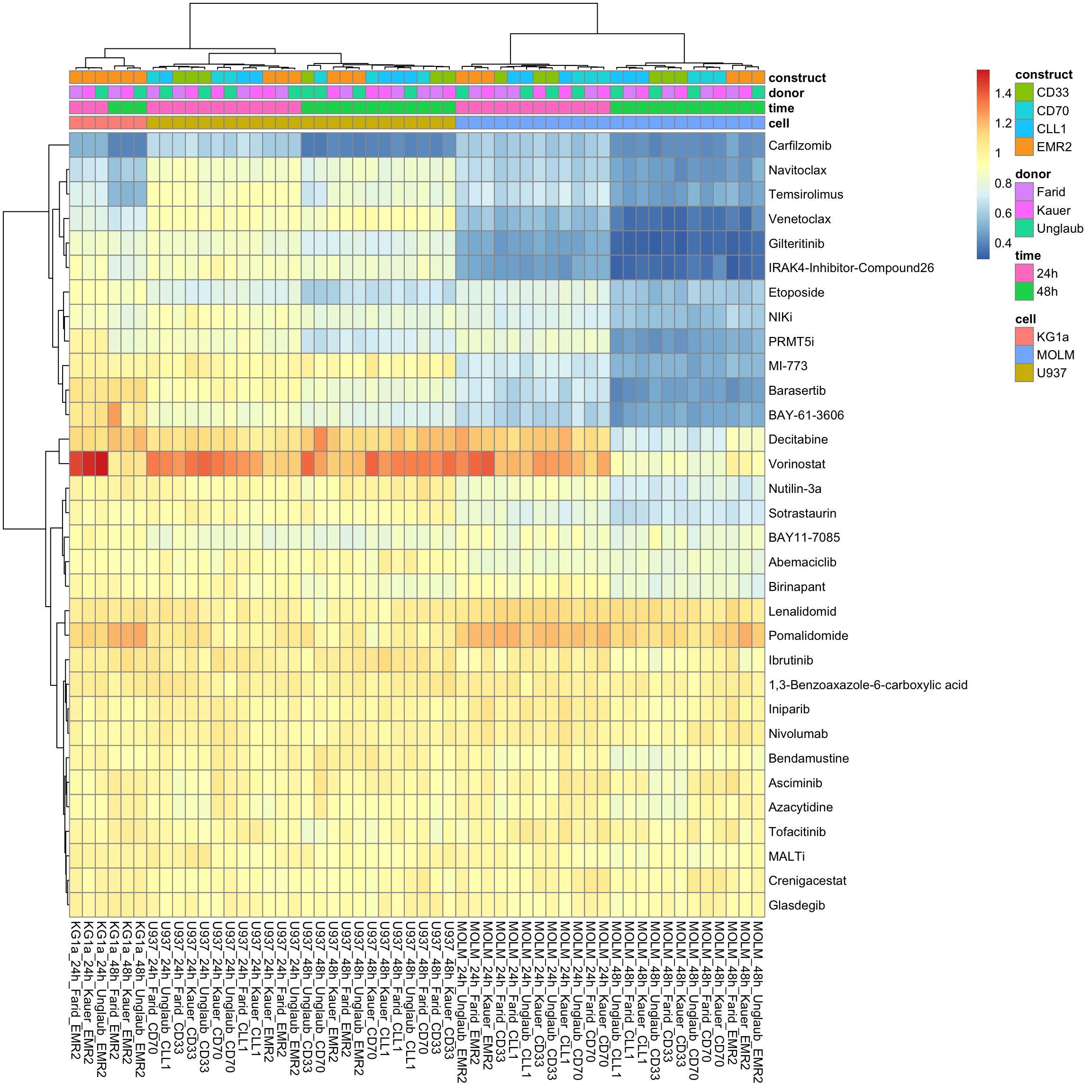
With row normalization, colores indicate row-wise z-scores
pheatmap::pheatmap(viabMat, annotation_col = colAnno, show_colnames = TRUE, clustering_method = "ward.D2", scale = "row")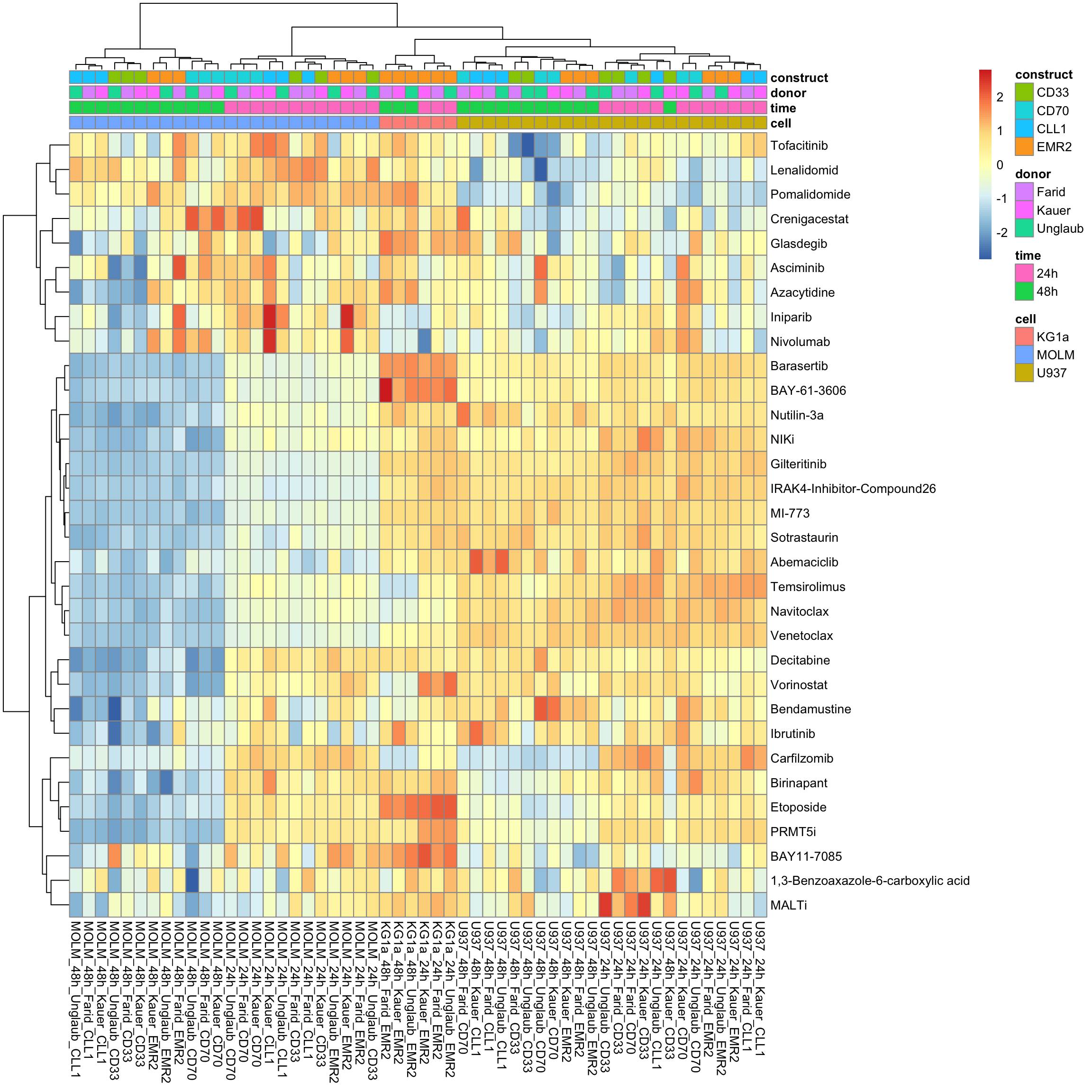
Visualize Drug + CAR effect
Dose-response curves
plotTab <- filter(screenData, Drug != "DMSO", Tcell == "CAR")

pList <- lapply(unique(sort(plotTab$cellTime)),function(nn) {
  eachTab <- filter(plotTab, cellTime == nn)
  ggplot(eachTab, aes(x=conc, y=normVal)) +
    geom_point() +
    geom_line(aes(group = donorConstruct, color = donorConstruct)) +
    facet_wrap(~Drug, scale = "free_x", ncol=4) +
    scale_x_log10() +
    xlab("Concentration") + ylab("Viability") +
    ggtitle(nn)
})

jyluMisc::makepdf(pList, "../docs/drugCAR_doseResponse.pdf", ncol=1, nrow=1, height = 15, width = 10)Heatmap of AUC of drug effect
aucTab <- filter(screenData, Drug != "DMSO", Tcell == "CAR") %>%
  group_by(cell, time, donor, construct, Drug, plateID) %>%
  summarise(auc = calcAUC(normVal, conc)) %>% ungroup()

colAnno <- distinct(aucTab, plateID, cell, time, donor, construct) %>%
  column_to_rownames("plateID") %>% data.frame()

viabMat <- aucTab %>% select(plateID, auc, Drug) %>%
  pivot_wider(names_from = plateID, values_from = auc) %>%
  column_to_rownames("Drug") %>% as.matrix()
Without row normalization, colores indicate viability
pheatmap::pheatmap(viabMat, annotation_col = colAnno, show_colnames = TRUE, clustering_method = "ward.D2")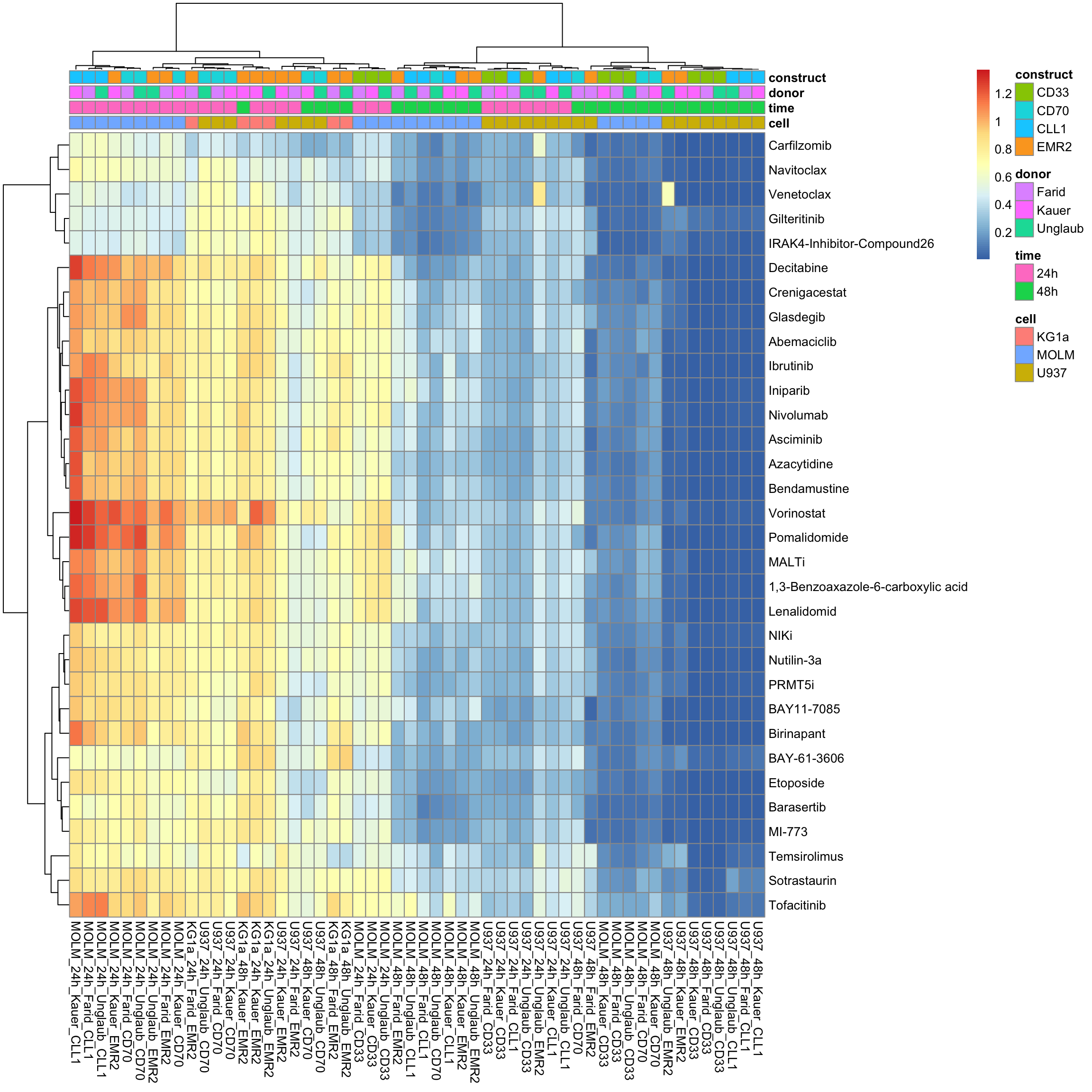
With row normalization, colores indicate row-wise z-scores
pheatmap::pheatmap(viabMat, annotation_col = colAnno, show_colnames = TRUE, clustering_method = "ward.D2", scale = "row")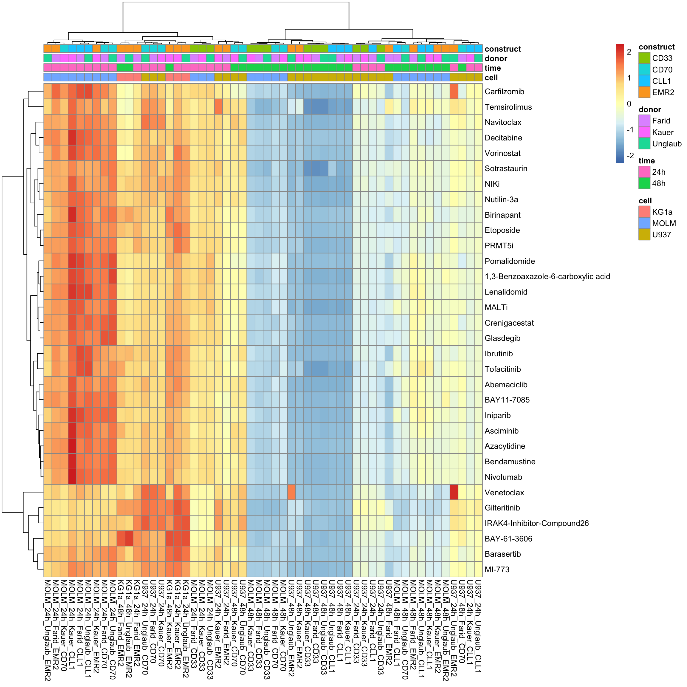
sessionInfo()R version 4.2.0 (2022-04-22)
Platform: x86_64-apple-darwin17.0 (64-bit)
Running under: macOS Big Sur/Monterey 10.16
Matrix products: default
BLAS: /Library/Frameworks/R.framework/Versions/4.2/Resources/lib/libRblas.0.dylib
LAPACK: /Library/Frameworks/R.framework/Versions/4.2/Resources/lib/libRlapack.dylib
locale:
[1] en_US.UTF-8/en_US.UTF-8/en_US.UTF-8/C/en_US.UTF-8/en_US.UTF-8
attached base packages:
[1] stats graphics grDevices utils datasets methods base
other attached packages:
[1] gridExtra_2.3 forcats_0.5.1 stringr_1.4.1 dplyr_1.0.9
[5] purrr_0.3.4 readr_2.1.2 tidyr_1.2.0 tibble_3.1.8
[9] ggplot2_3.4.1 tidyverse_1.3.2 readxl_1.4.0
loaded via a namespace (and not attached):
[1] backports_1.4.1 fastmatch_1.1-3
[3] drc_3.0-1 jyluMisc_0.1.5
[5] workflowr_1.7.0 igraph_1.3.4
[7] shinydashboard_0.7.2 splines_4.2.0
[9] BiocParallel_1.30.3 GenomeInfoDb_1.32.2
[11] TH.data_1.1-1 digest_0.6.30
[13] htmltools_0.5.4 fansi_1.0.3
[15] magrittr_2.0.3 googlesheets4_1.0.0
[17] cluster_2.1.3 tzdb_0.3.0
[19] limma_3.52.2 modelr_0.1.8
[21] matrixStats_0.62.0 sandwich_3.0-2
[23] piano_2.12.0 colorspace_2.0-3
[25] rvest_1.0.2 haven_2.5.0
[27] xfun_0.31 crayon_1.5.2
[29] RCurl_1.98-1.7 jsonlite_1.8.3
[31] survival_3.4-0 zoo_1.8-10
[33] glue_1.6.2 survminer_0.4.9
[35] gtable_0.3.0 gargle_1.2.0
[37] zlibbioc_1.42.0 XVector_0.36.0
[39] DelayedArray_0.22.0 car_3.1-0
[41] BiocGenerics_0.42.0 abind_1.4-5
[43] scales_1.2.0 pheatmap_1.0.12
[45] mvtnorm_1.1-3 DBI_1.1.3
[47] relations_0.6-12 rstatix_0.7.0
[49] Rcpp_1.0.9 plotrix_3.8-2
[51] xtable_1.8-4 km.ci_0.5-6
[53] stats4_4.2.0 DT_0.23
[55] htmlwidgets_1.5.4 httr_1.4.3
[57] fgsea_1.22.0 RColorBrewer_1.1-3
[59] gplots_3.1.3 ellipsis_0.3.2
[61] pkgconfig_2.0.3 farver_2.1.1
[63] sass_0.4.2 dbplyr_2.2.1
[65] utf8_1.2.2 tidyselect_1.1.2
[67] labeling_0.4.2 rlang_1.0.6
[69] later_1.3.0 munsell_0.5.0
[71] cellranger_1.1.0 tools_4.2.0
[73] visNetwork_2.1.0 cachem_1.0.6
[75] cli_3.4.1 generics_0.1.3
[77] broom_1.0.0 evaluate_0.15
[79] fastmap_1.1.0 yaml_2.3.5
[81] knitr_1.39 fs_1.5.2
[83] survMisc_0.5.6 caTools_1.18.2
[85] mime_0.12 slam_0.1-50
[87] xml2_1.3.3 compiler_4.2.0
[89] rstudioapi_0.13 ggsignif_0.6.3
[91] marray_1.74.0 reprex_2.0.1
[93] bslib_0.4.1 stringi_1.7.8
[95] highr_0.9 lattice_0.20-45
[97] Matrix_1.5-4 KMsurv_0.1-5
[99] shinyjs_2.1.0 vctrs_0.5.2
[101] pillar_1.8.0 lifecycle_1.0.3
[103] jquerylib_0.1.4 data.table_1.14.8
[105] cowplot_1.1.1 bitops_1.0-7
[107] httpuv_1.6.6 GenomicRanges_1.48.0
[109] R6_2.5.1 promises_1.2.0.1
[111] KernSmooth_2.23-20 IRanges_2.30.0
[113] codetools_0.2-18 MASS_7.3-58
[115] gtools_3.9.3 exactRankTests_0.8-35
[117] assertthat_0.2.1 SummarizedExperiment_1.26.1
[119] rprojroot_2.0.3 withr_2.5.0
[121] multcomp_1.4-19 S4Vectors_0.34.0
[123] GenomeInfoDbData_1.2.8 parallel_4.2.0
[125] hms_1.1.1 grid_4.2.0
[127] rmarkdown_2.14 MatrixGenerics_1.8.1
[129] carData_3.0-5 googledrive_2.0.0
[131] ggpubr_0.4.0 git2r_0.30.1
[133] maxstat_0.7-25 sets_1.0-21
[135] Biobase_2.56.0 shiny_1.7.4
[137] lubridate_1.8.0