Identify additive effect between drug and CAR-T treatment using highest single agent model (with highly toxic single angent effect removed)
Junyan Lu
Last updated: 2023-06-15
Checks: 5 1
Knit directory: combiCART/analysis/
This reproducible R Markdown analysis was created with workflowr (version 1.7.0). The Checks tab describes the reproducibility checks that were applied when the results were created. The Past versions tab lists the development history.
Great job! The global environment was empty. Objects defined in the global environment can affect the analysis in your R Markdown file in unknown ways. For reproduciblity it’s best to always run the code in an empty environment.
The command set.seed(20221110) was run prior to running
the code in the R Markdown file. Setting a seed ensures that any results
that rely on randomness, e.g. subsampling or permutations, are
reproducible.
Great job! Recording the operating system, R version, and package versions is critical for reproducibility.
Nice! There were no cached chunks for this analysis, so you can be confident that you successfully produced the results during this run.
Great job! Using relative paths to the files within your workflowr project makes it easier to run your code on other machines.
Tracking code development and connecting the code version to the
results is critical for reproducibility. To start using Git, open the
Terminal and type git init in your project directory.
This project is not being versioned with Git. To obtain the full
reproducibility benefits of using workflowr, please see
?wflow_start.
Here, additive means if a observed combination effect is stronger than the highest effect of either of drug or CAR-T alone, it will be considered as candidate. The model is less stringent than Bliss independence model, where only true synergism will be considered. This model will identify both synergism and simple additive effect
Load packages and dataset
library(readxl)
library(tidyverse)
knitr::opts_chunk$set(warning = FALSE, message = FALSE)
source("../code/helper.R")
load("../output/screenData.RData")
Use drug effect normalized by NT only wells for the down-stream analysis
screenData <- mutate(screenData, normVal = normVal.NT)Calculate combination index using highest agent model
Get combination effect
comTab <- filter(screenData, Drug !="DMSO", Tcell == "CAR") %>%
  select(plateID, Drug, conc, normVal) %>%
  dplyr::rename(viabObs = normVal)

drugTab <- filter(screenData, Drug != "DMSO", Tcell == "NT") %>%
  select(plateID, Drug, conc, normVal) %>%
  dplyr::rename(viabDrug = normVal)

carTab <- filter(screenData, Drug == "DMSO", Tcell == "CAR") %>%
  select(plateID, normVal) %>% group_by(plateID) %>%
  summarise(viabCar = median(normVal))
synTab <- comTab %>% left_join(drugTab, by =c("plateID","Drug","conc")) %>%
left_join(carTab, by = "plateID") %>%
mutate(viabExp = ifelse(viabDrug < viabCar, viabDrug, viabCar)) %>%
mutate(CI = viabObs-viabExp,
logCI = log10(viabObs/viabExp))Remove combination if single agent effect (either drug or CAR) is already very strong (viability < 0.2) if all three donors
excludeTab <- synTab %>% mutate(toxic = (viabDrug < 0.2 | viabCar < 0.2)) %>%
  left_join(distinct(screenData, plateID, construct, cellTime), by = "plateID") %>%
  group_by(cellTime, construct, Drug, conc) %>% summarise(n=sum(toxic)) %>% ungroup()
synTab <- left_join(synTab, distinct(screenData, plateID, construct, cellTime), by = "plateID") %>%
  left_join(excludeTab, by =c("cellTime","construct","Drug","conc")) %>%
  filter(n<3) %>%
  dplyr::select(-cellTime, -construct, -n)
Visualize synergistic index per concentration in a heatmap
24 hours
plotTab <- left_join(synTab, distinct(screenData, plateID, time, construct)) %>%
filter(time == "24h") %>%
arrange(construct, plateID) %>%
mutate(plateID = factor(plateID, levels = unique(plateID)))
ggplot(plotTab, aes(x=factor(conc), y=plateID, fill = CI)) +
geom_tile() +
facet_wrap(~Drug, ncol=4, scale = "free_x") +
scale_fill_gradient2(low ="red",high="blue",mid="white") 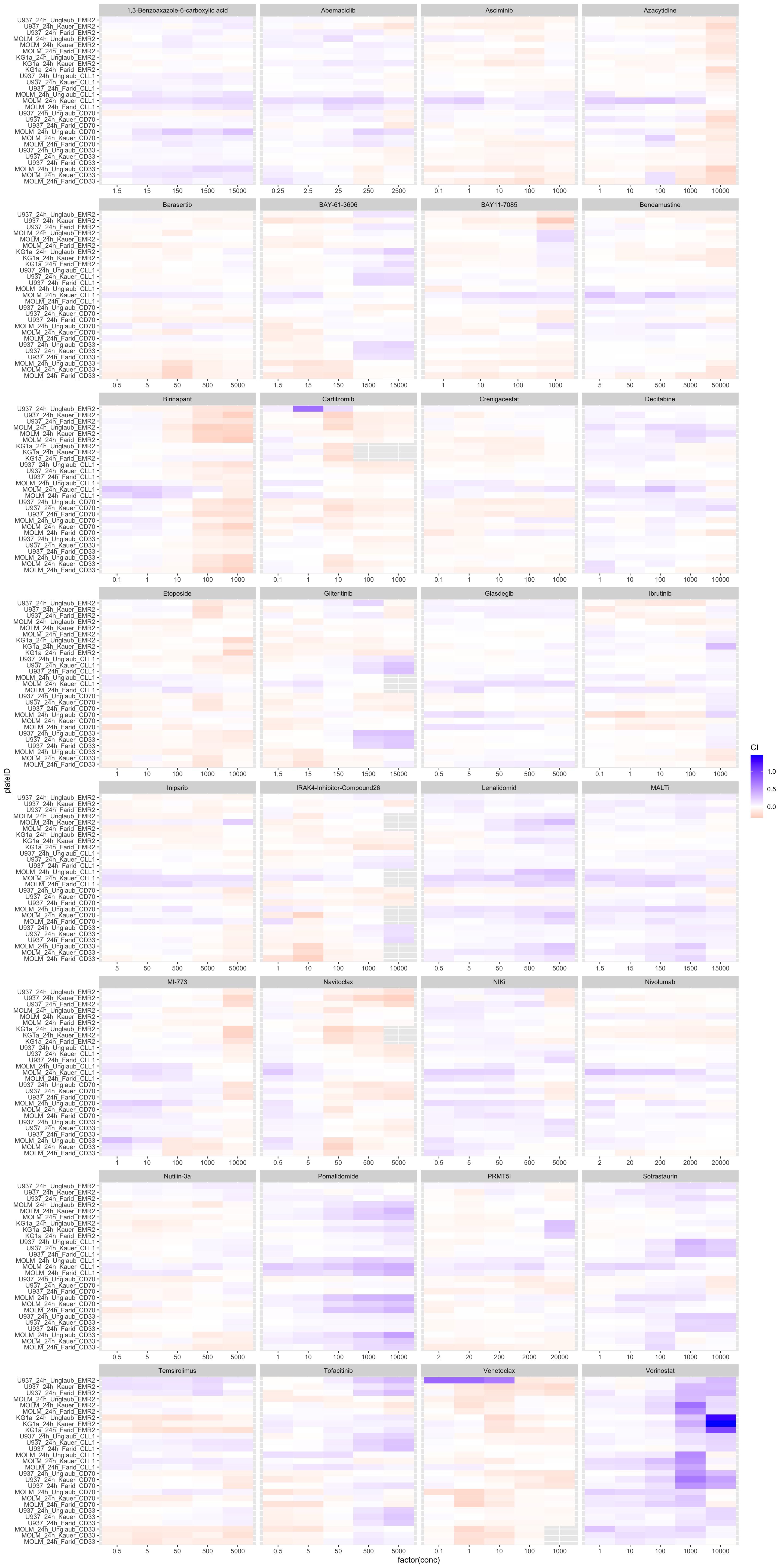 **Positive CI indicates antagonistic effect and negative CI indicates
synergistic effect)
**Positive CI indicates antagonistic effect and negative CI indicates
synergistic effect)
48 hours
plotTab <- left_join(synTab, distinct(screenData, plateID, time, construct)) %>%
  filter(time == "48h") %>%
  arrange(construct, plateID) %>%
  mutate(plateID = factor(plateID, levels = unique(plateID)))

ggplot(plotTab, aes(x=factor(conc), y=plateID, fill = CI)) +
  geom_tile() +
  facet_wrap(~Drug, ncol=4, scale = "free_x") +
scale_fill_gradient2(low ="red",high="blue",mid="white") 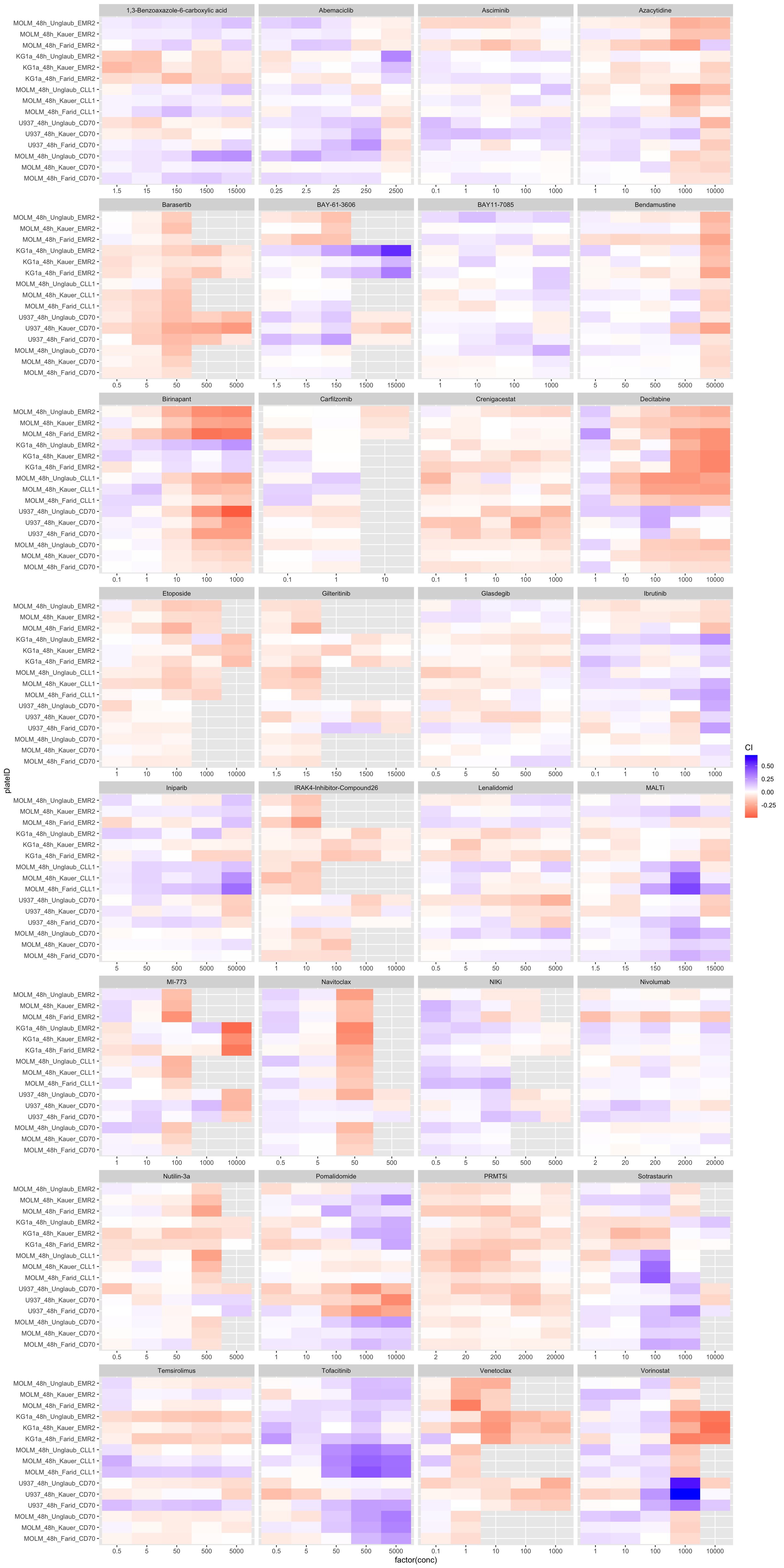
Rank drugs based on their median combination index (for every concentration)
Only drugs with median CI < 0 (synergistic or additive) are shown
24 hours
plotTab <- left_join(synTab, distinct(screenData, plateID, time, construct)) %>%
  left_join(distinct(screenData, Drug, conc, concStep), by = c("Drug","conc")) %>%
  filter(time == "24h") %>%
  mutate(drugConc = paste0(Drug,"_", conc)) %>%
  group_by(drugConc) %>% mutate(medVal = median(CI)) %>% arrange(medVal) %>%
  ungroup()%>%
  mutate(drugConc = factor(drugConc, levels = unique(drugConc))) %>%
  filter(medVal < 0)

ggplot(plotTab, aes(x=drugConc, y=CI, fill = concStep)) +
  ggbeeswarm::geom_quasirandom(shape = 21, alpha =0.5) +
  stat_summary(fun.y = median, fun.ymin = median, fun.ymax = median, color = "darkred",
          geom = "crossbar", width = 0.5) +
  coord_cartesian(ylim=c(-0.5,0.5)) +
  geom_hline(yintercept = 0, linetype = "dashed") +
theme(axis.text.x = element_text(angle = 90, hjust = 1, vjust = 0.5)) 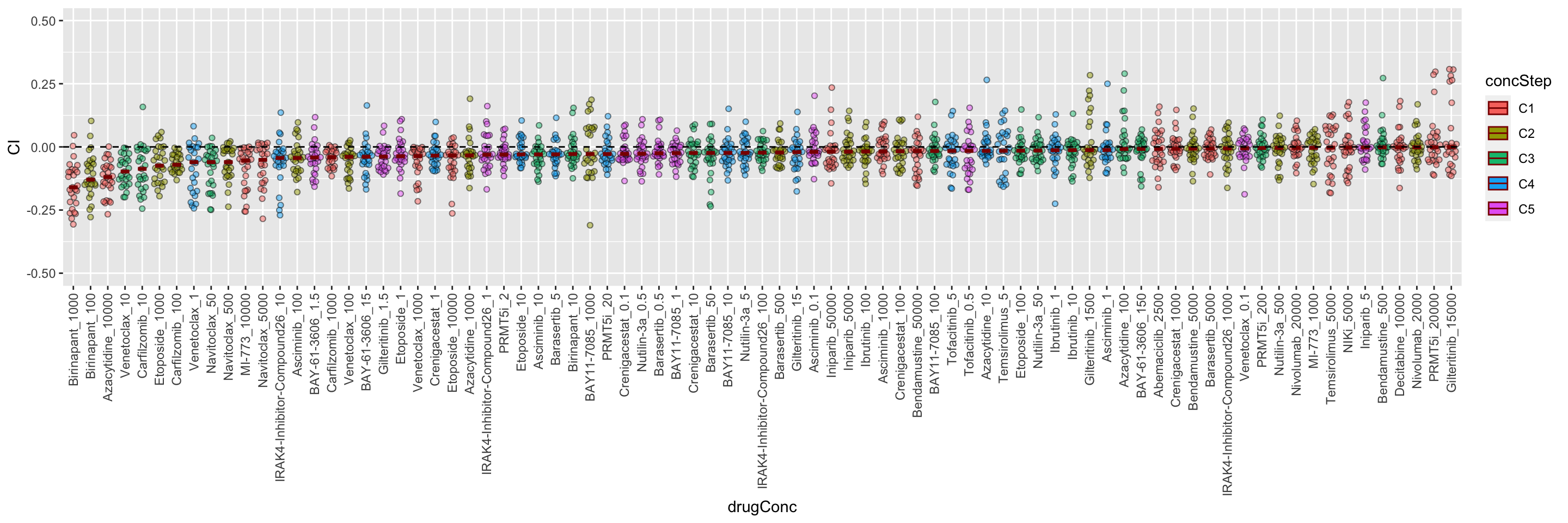
48 hours
plotTab <- left_join(synTab, distinct(screenData, plateID, time, construct)) %>%
  left_join(distinct(screenData, Drug, conc, concStep), by = c("Drug","conc")) %>%
  filter(time == "48h") %>%
  mutate(drugConc = paste0(Drug,"_", conc)) %>%
  group_by(drugConc) %>% mutate(medVal = median(CI)) %>% arrange(medVal) %>%
  ungroup()%>%
  mutate(drugConc = factor(drugConc, levels = unique(drugConc))) %>%
  filter(medVal < 0)

ggplot(plotTab, aes(x=drugConc, y=CI, fill = concStep)) +
  ggbeeswarm::geom_quasirandom(shape = 21, alpha =0.5) +
  stat_summary(fun.y = median, fun.ymin = median, fun.ymax = median, color = "darkred",
          geom = "crossbar", width = 0.5) +
  coord_cartesian(ylim=c(-0.5,0.5)) +
  geom_hline(yintercept = 0, linetype = "dashed") +
theme(axis.text.x = element_text(angle = 90, hjust = 1, vjust = 0.5)) 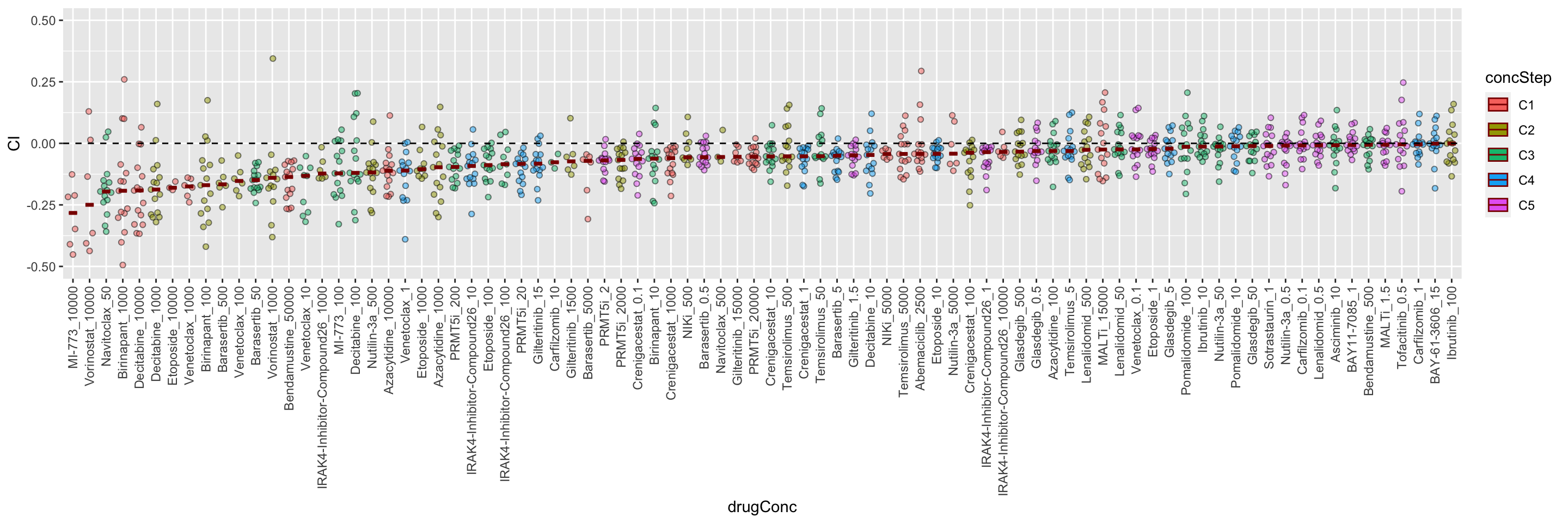
Summarise CI
Calculate synergistic and antagonistic effect separately, using a similar way as bayesyngergy package
sumSyn <- function(viabExp, viabObs) {
  tab <- tibble(viabExp=viabExp, viabObs = viabObs) %>%
    mutate(syn = min(0, viabObs - viabExp),
           anta = max(0, viabObs - viabExp))
  return(tibble(syn = sum(tab$syn,na.rm = TRUE), anta = sum(tab$anta,na.rm = TRUE)))
}

ciTabSum <- group_by(synTab, plateID, Drug) %>% nest() %>%
  mutate(res = map(data, ~sumSyn(.$viabExp, .$viabObs))) %>%
  unnest(res) %>% select(-data)
Visualization of additive and antagoistic effect
plotSynScatter <- function(plotTab, labelPercent = 0.05) {

  synCut <-  quantile(plotTab$syn, labelPercent)
  antaCut <- quantile(plotTab$anta, 1-labelPercent)

  plotTabSyn <- plotTab %>% mutate(labelText = ifelse(syn < synCut, plateID,""), type = "Additive effect") %>%
    mutate(score = syn)
  plotTabAnta <- plotTab %>% mutate(labelText = ifelse(anta > antaCut, plateID,""), type = "Antagonistic effect") %>%
    mutate(score = anta)
  plotComb <- bind_rows(plotTabSyn, plotTabAnta)

  p <- ggplot(plotComb, aes(x=Drug, y=score, label = labelText)) +
    geom_point(aes(col= type), alpha=0.5) + ggrepel::geom_text_repel(max.overlaps = Inf) +
    theme_bw() +
    theme(axis.text.x = element_text(angle = 90, hjust=1, vjust = 0.5)) +
    scale_color_manual(values = c("Additive effect" = "red", "Antagonistic effect" = "blue")) +
    #facet_wrap(~type, ncol=2)
    ylab("Combination Score") + xlab("") +
    theme(legend.position = "bottom")
  return(p)
}
Scatter plot
Top 5% synergistics or antagonistic effect are labelled.
plotSynScatter(ciTabSum,0.01)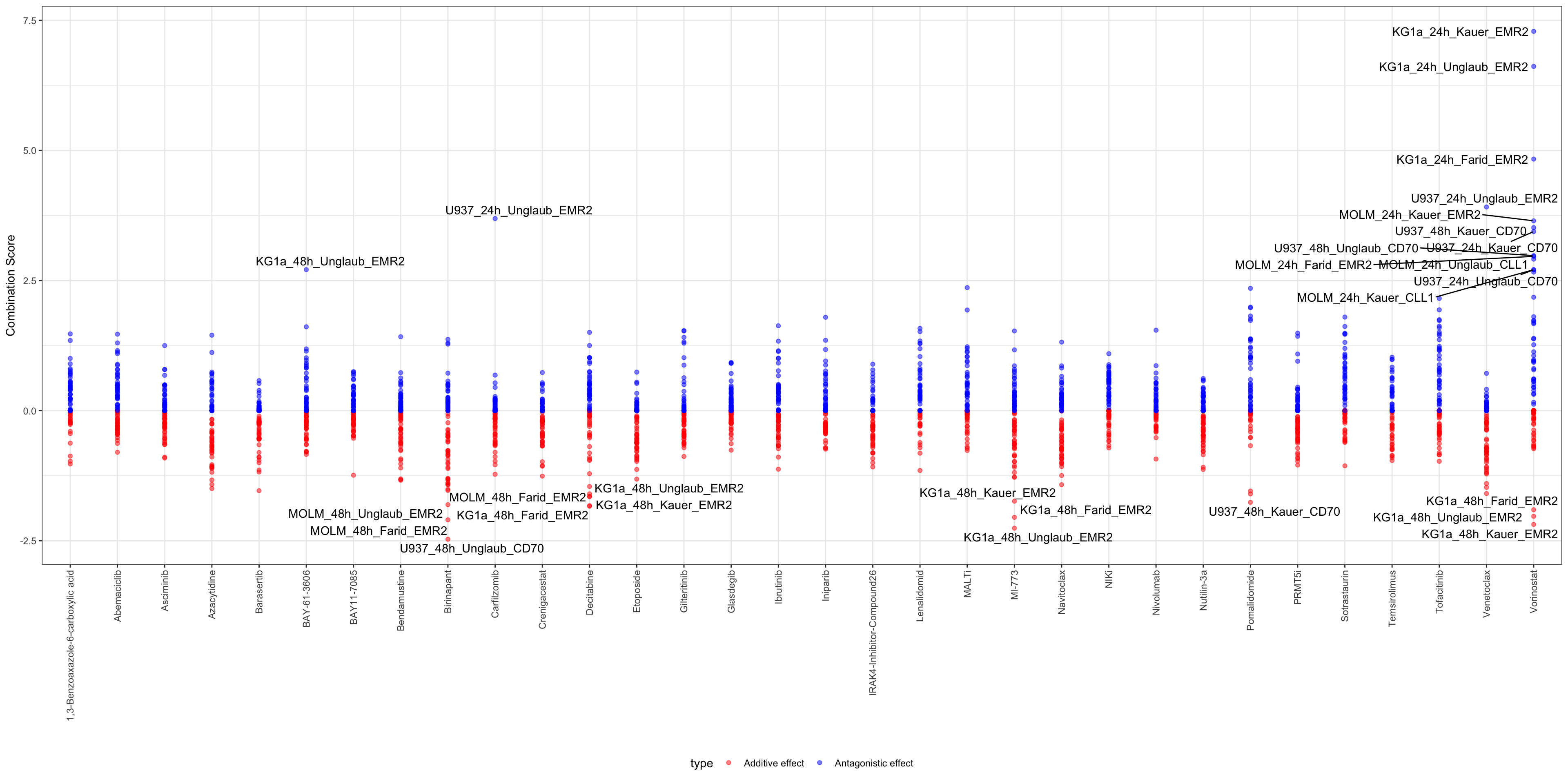
Matrix visualization
plotSynMatrix <- function(ciTabSum, cut1 = 0.1, cut2 = 0.2) {
  synCut1 <-  quantile(ciTabSum$syn, cut1)
  antaCut1 <- quantile(ciTabSum$anta, 1-cut1)
  synCut2 <-  quantile(ciTabSum$syn, cut2)
  antaCut2 <- quantile(ciTabSum$anta, 1-cut2)

  synOrder <- hcOrder(ciTabSum$Drug, ciTabSum$plateID, ciTabSum$syn)
  antaOrder <- hcOrder(ciTabSum$Drug, ciTabSum$plateID, ciTabSum$anta)

  plotTabSyn <- ciTabSum %>% mutate(degree = case_when(
    syn <= synCut1 ~ "**",
    syn <= synCut2 ~ "*",
    TRUE ~ ""
  )) %>% mutate(Drug = factor(Drug, levels = synOrder$row),
                plateID = factor(plateID, levels = synOrder$col))

  plotTabAnta <- ciTabSum %>% mutate(degree = case_when(
    anta >= antaCut1 ~ "**",
    anta >= antaCut2 ~ "*",
    TRUE ~ ""
  )) %>% mutate(Drug = factor(Drug, levels = antaOrder$row),
                plateID = factor(plateID, levels = antaOrder$col))

  p1 <- ggplot(plotTabSyn, aes(x=Drug, y=plateID, label = degree)) +
    geom_tile(aes(fill = syn)) +
    scale_fill_gradient(low="red", high="white", name = "syngergy") +
    geom_text() + ggtitle("Additive effect") +
    theme(axis.text.x = element_text(angle = 90, hjust=1, vjust=0.5))

  p2 <- ggplot(plotTabAnta, aes(x=Drug, y=plateID, label = degree)) +
    geom_tile(aes(fill = anta)) +
    scale_fill_gradient(low="white", high="blue", name = "antagonism") +
    geom_text() + ggtitle("Antagonistic effect") +
    theme(axis.text.x = element_text(angle = 90, hjust=1, vjust=0.5))

  p <- cowplot::plot_grid(p2, p1, ncol=2)
  return(p)
}
plotSynMatrix(ciTabSum, 0.01, 0.05)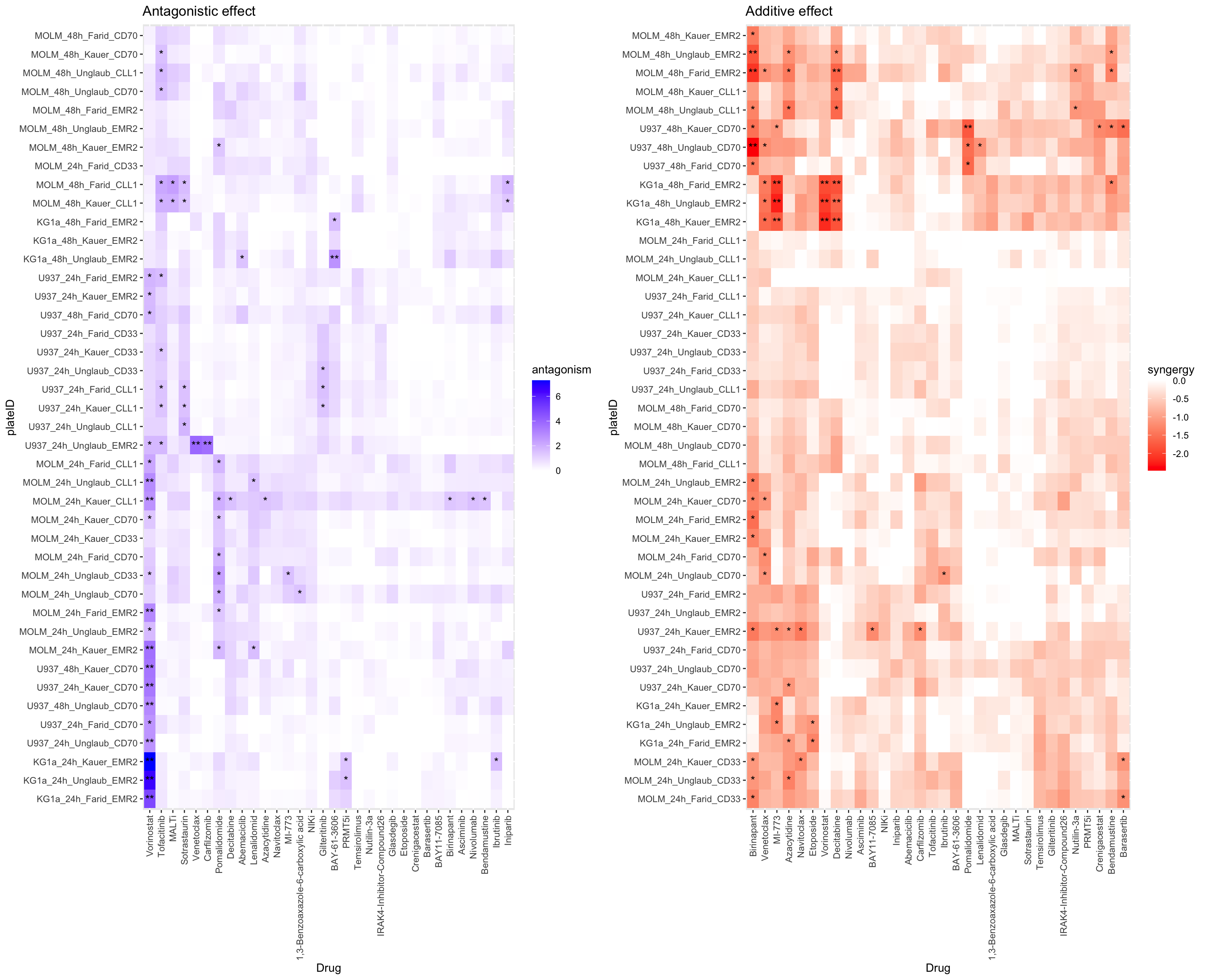
Plot combination curve for each drug, witin each drug, cell models are ranked based on CI
drugs <- sort(unique(synTab$Drug))

pList <- lapply(drugs, function(eachDrug) {
  ciRank <- filter(ciTabSum, Drug==eachDrug) %>%
    arrange(syn)

  plotTab <- filter(synTab, Drug == eachDrug) %>%
    select(plateID, Drug, conc, viabDrug, viabCar, viabObs) %>%
    pivot_longer(-c("plateID","Drug","conc"), names_to = "type", values_to = "viab") %>%
    mutate(plateID = factor(plateID, levels = ciRank$plateID)) %>%
    mutate(type = factor(type, levels = c("viabDrug","viabCar","viabObs")))

  ggplot(plotTab, aes(x=factor(conc), y=viab, group=type)) +
    geom_line(aes(col = type)) +
    facet_wrap(~plateID,ncol=5) +
    #scale_linetype_manual(values = c(combine = "solid", `single` = "dotted"), name = "combination") +
    scale_color_manual(values =c(viabDrug = "orange", viabCar="darkgreen",
                                 viabObs="blue"),
                       labels=c("drug only ","Car only", "observed effect"),
                       name = "treatment") +
    ggtitle(eachDrug) +
    ylab("Viability") + xlab("Concentration")
})
jyluMisc::makepdf(pList, "../docs/combo_effect_additive_noToxic.pdf",nrow = 1, ncol = 1, height = 18, width = 12)Test for significant combination effect in cells using paired t-test (consider donors as replicates)
Test for each individual concentration
testTab <- synTab %>%
  left_join(distinct(screenData, plateID, cell, time, construct, donor), by = "plateID") %>%
  mutate(cellTimeConst = paste0(cell,"_",time,"_",construct))

resTab <- group_by(testTab, cell, time, construct, Drug, conc, cellTimeConst) %>% nest() %>%
  mutate(m = map(data, ~t.test(.$viabObs, .$viabExp, paired=TRUE))) %>%
  mutate(res = map(m, broom::tidy)) %>%
  unnest(res) %>%
  select(Drug, conc, cell, time, construct, cellTimeConst, estimate, p.value) %>%
  arrange(p.value) %>% ungroup() %>%
  mutate(p.adj = p.adjust(p.value, method ="BH"))
P-value heatmap for summarising the results
24 hours
Heatmaps
resSub <- filter(resTab, time == "24h")
pList <- lapply(unique(resSub$Drug), function(dd) {
plotTab <- filter(resSub, Drug == dd) %>%
mutate(effect = ifelse(estimate >0, "antagonisim","synergy"),
ifSig = case_when(p.value <= 0.01 & p.adj > 0.1 ~ "*",
p.adj <= 0.1 ~ "**",
p.value > 0.01 ~ "")) %>%
arrange(construct,cellTimeConst) %>%
mutate(cellTimeConst = factor(cellTimeConst, levels = unique(cellTimeConst)))
pHeat <- ggplot(plotTab, aes(x=factor(conc),y=cellTimeConst, fill = estimate)) +
geom_tile() +
geom_text(aes(label = ifSig), vjust =0.5) +
scale_x_discrete(expand = c(0,0)) + scale_y_discrete(expand = c(0,0)) +
scale_fill_gradient2(low ="red",high="blue",mid="white", midpoint = 0, name = "CI") +
theme_minimal() +
ggtitle(dd) +theme(plot.title = element_text(size = 14, face = "bold", hjust = 0.5),
axis.text.x = element_blank(), panel.grid = element_blank(),
axis.title.x = element_blank()) +
ylab("")
pBox <- ggplot(plotTab, aes(x=factor(conc), y=estimate)) +
geom_point(shape =1,size=2) +
stat_summary(fun.y = median, fun.ymin = median, fun.ymax = median, color = "darkred",
geom = "crossbar", width = 0.5) +
geom_hline(yintercept = 0, linetype = "dashed") +
ylab("Average CI") + xlab("Concentration")+
theme_bw()
cowplot::plot_grid(pHeat, pBox, align = "v", axis ="lr",ncol=1, rel_heights = c(1,0.6))
})
cowplot::plot_grid(plotlist = pList, ncol=4)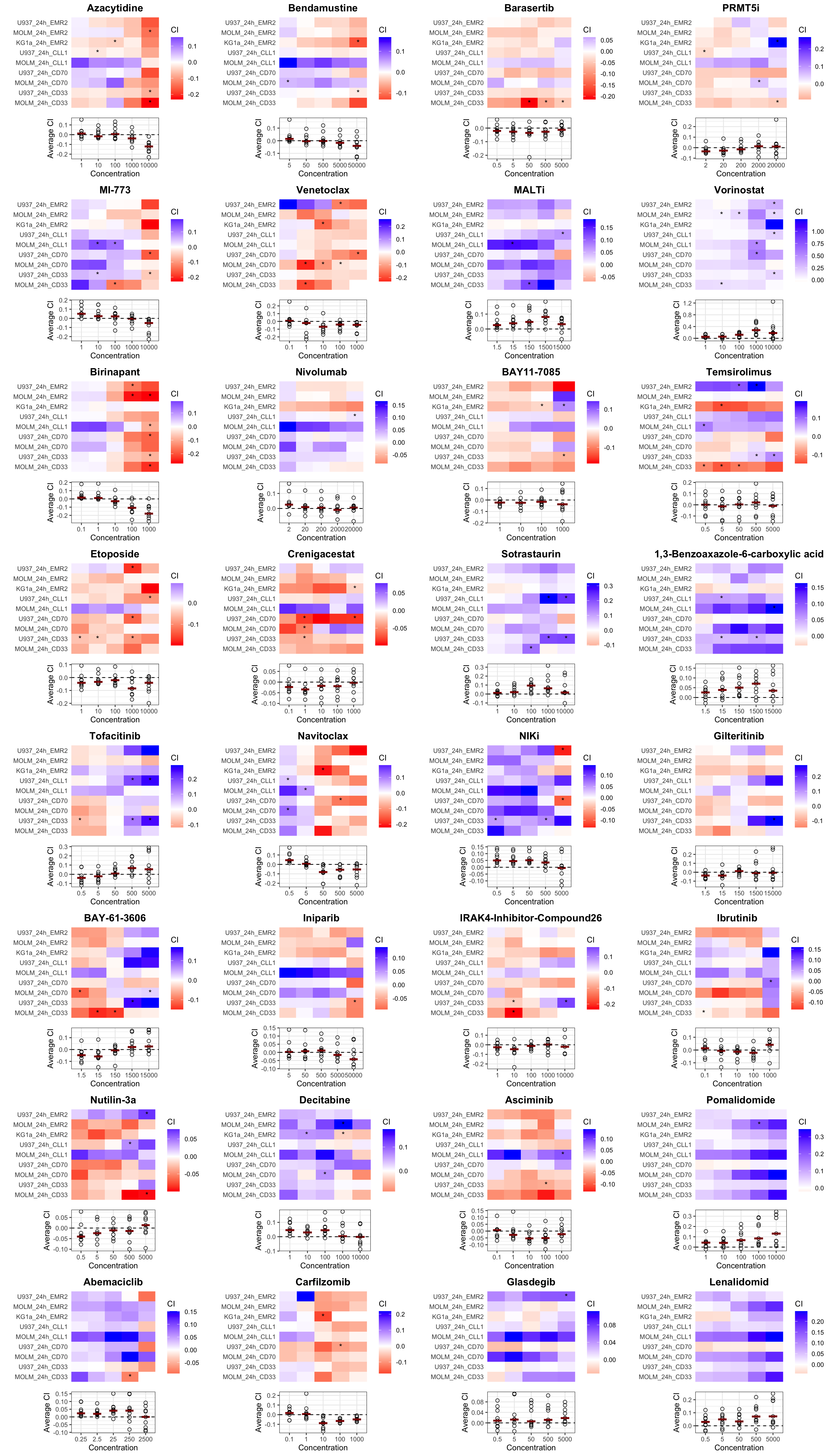 one star indicates P value < 0.01, two starts indicate FDR
< 10%
one star indicates P value < 0.01, two starts indicate FDR
< 10%
negative CI indicates synergy, positive CI indicates
antagonism
The plot below the heatmap shows the median CI for each
concentration
48 hours
Heatmaps
resSub <- filter(resTab, time == "48h")

pList <- lapply(unique(resSub$Drug), function(dd) {
  plotTab <- filter(resSub, Drug == dd) %>%
    mutate(effect = ifelse(estimate >0, "antagonisim","synergy"),
           ifSig = case_when(p.value <= 0.01 & p.adj > 0.1 ~ "*",
                             p.adj <= 0.1 ~ "**",
                             p.value > 0.01 ~ "")) %>%
    arrange(construct,cellTimeConst) %>%
    mutate(cellTimeConst = factor(cellTimeConst, levels = unique(cellTimeConst)))

  pHeat <- ggplot(plotTab, aes(x=factor(conc),y=cellTimeConst, fill = estimate)) +
    geom_tile() +
    geom_text(aes(label = ifSig), vjust =0.5) +
    scale_x_discrete(expand = c(0,0)) + scale_y_discrete(expand = c(0,0)) +
    scale_fill_gradient2(low ="red",high="blue",mid="white", midpoint = 0, name = "CI") +
    theme_minimal() +
    ggtitle(dd) +theme(plot.title = element_text(size = 14, face = "bold", hjust = 0.5),
                       axis.text.x = element_blank(), panel.grid = element_blank(),
                       axis.title.x = element_blank()) +
    ylab("")


  pBox <- ggplot(plotTab, aes(x=factor(conc), y=estimate)) +
    geom_point(shape =1,size=2) +
    stat_summary(fun.y = median, fun.ymin = median, fun.ymax = median, color = "darkred",
                 geom = "crossbar", width = 0.5) +
    geom_hline(yintercept = 0, linetype = "dashed") +
    ylab("Average CI") + xlab("Concentration")+
    theme_bw()

  cowplot::plot_grid(pHeat, pBox, align = "v", axis ="lr",ncol=1, rel_heights = c(1,0.6))
})

cowplot::plot_grid(plotlist = pList, ncol=4)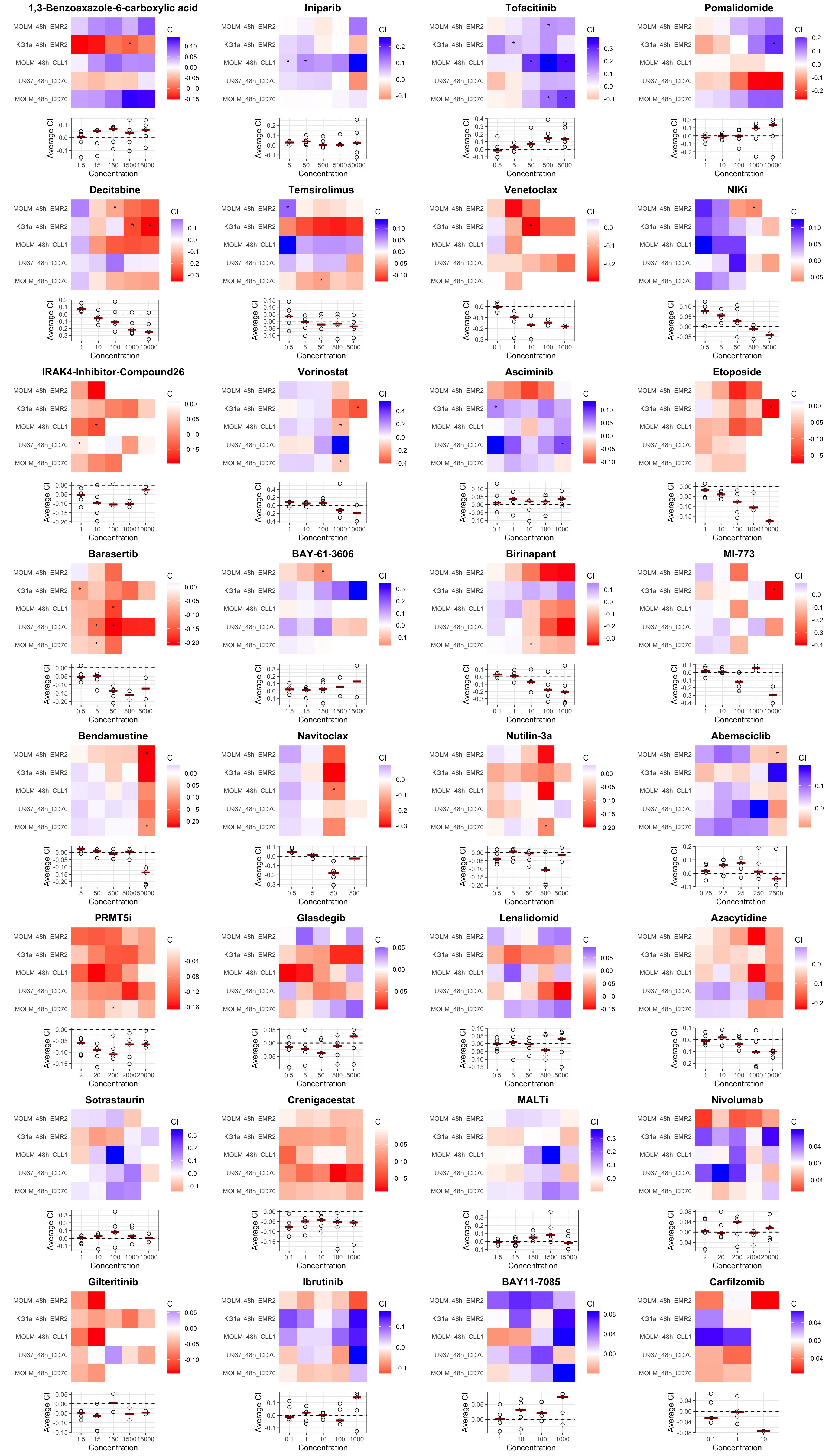
Test for AUC of summarise effect across concentrations
testTab <- synTab %>%
  left_join(distinct(screenData, plateID, cell, time, construct, donor), by = "plateID") %>%
  mutate(cellTimeConst = paste0(cell,"_",time,"_",construct)) %>%
  group_by(Drug, cellTimeConst, donor) %>%
  summarise(viabObs = calcAUC(viabObs, conc),
            viabExp = calcAUC(viabExp, conc))

resTab <- group_by(testTab, Drug, cellTimeConst) %>% nest() %>%
  mutate(m = map(data, ~t.test(.$viabObs, .$viabExp, paired=TRUE))) %>%
  mutate(res = map(m, broom::tidy)) %>%
  unnest(res) %>%
  select(Drug, cellTimeConst, estimate, p.value) %>%
  arrange(p.value) %>% ungroup() %>%
  mutate(p.adj = p.adjust(p.value, method ="BH"))
P-value heatmap for summarising the results
plotTab <- resTab %>%
mutate(effect = ifelse(estimate >0, "antagonism","synergy"),
ifSig = case_when(p.value <= 0.01 & p.adj > 0.1 ~ "*",
p.adj <= 0.1 ~ "**",
p.value > 0.01 ~ ""))
ggplot(plotTab, aes(x=Drug ,y=cellTimeConst, fill = estimate)) +
geom_tile() +
geom_text(aes(label = ifSig), vjust =0.5) +
scale_fill_gradient2(low ="red",high="blue",mid="white", midpoint = 0, name = "CI") +
theme(axis.text.x = element_text(angle = 90, hjust=1, vjust = 0.5))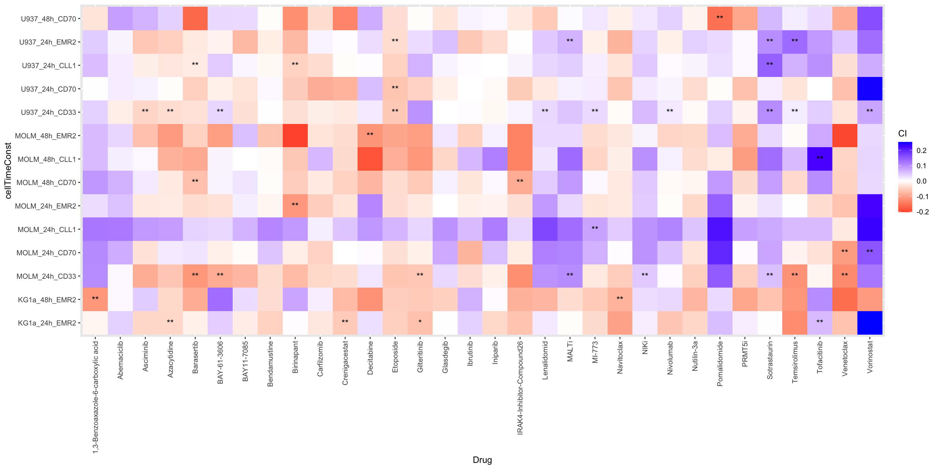 one star indicates P value < 0.01, two starts indicate FDR
< 10% (adj P value < 0.1)
one star indicates P value < 0.01, two starts indicate FDR
< 10% (adj P value < 0.1)
negative CI indicates synergy, positive CI indicates
antagonism
Volcano plot
plotTab <- resTab %>%
mutate(effect = ifelse(p.adj <= 0.1,
ifelse(estimate > 0, "antagonism","synergy"),
"n.s.")) %>%
mutate(labText = cellTimeConst)
ggplot(plotTab, aes(x=estimate ,y=-log10(p.value), color = effect)) +
geom_point() +
ggrepel::geom_text_repel(data = filter(plotTab, p.adj <=0.1, estimate <0), aes(label = labText), max.overlaps = Inf) +
scale_color_manual(values = c(synergy = "red", antagonism = "blue", "n.s." = "grey50")) +
theme_bw() +
xlab("Average CI") +
facet_wrap(~Drug)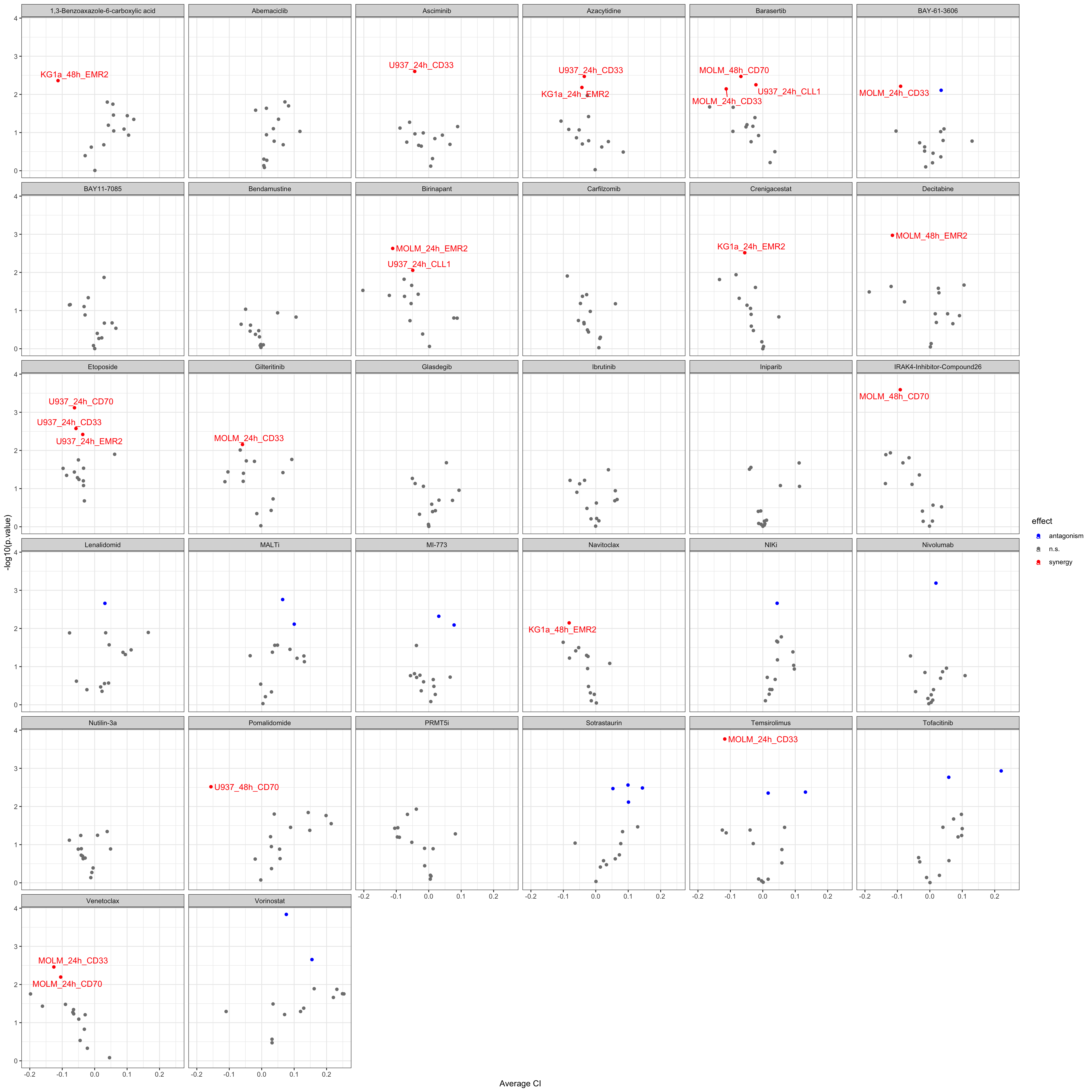 adj P-value < 0.05 (5% FDR) are colored
Line plots of significant pairs (10% FDR)
resTab.sig <- filter(plotTab, estimate < 0, p.adj < 0.1)

pList <- lapply(seq(nrow(resTab.sig)), function(i) {
  rec <- resTab.sig[i,]
  eachTab <- filter(testTab, Drug == rec$Drug, cellTimeConst == rec$cellTimeConst) %>%
    pivot_longer(c("viabObs","viabExp"), names_to = "type", values_to = "value") %>%
    mutate(type = ifelse(type == "viabObs", "observed","expected"))
  ggplot(eachTab, aes(x=type, y=value, col = donor)) +
    geom_point() +
    geom_line(aes(group =donor, col = donor)) +
    xlab("") + ylab("Viability") +
    ggtitle(sprintf("%s in %s", rec$Drug, rec$cellTimeConst)) +
    theme(legend.position = "bottom")
})

cowplot::plot_grid(plotlist = pList, ncol=4)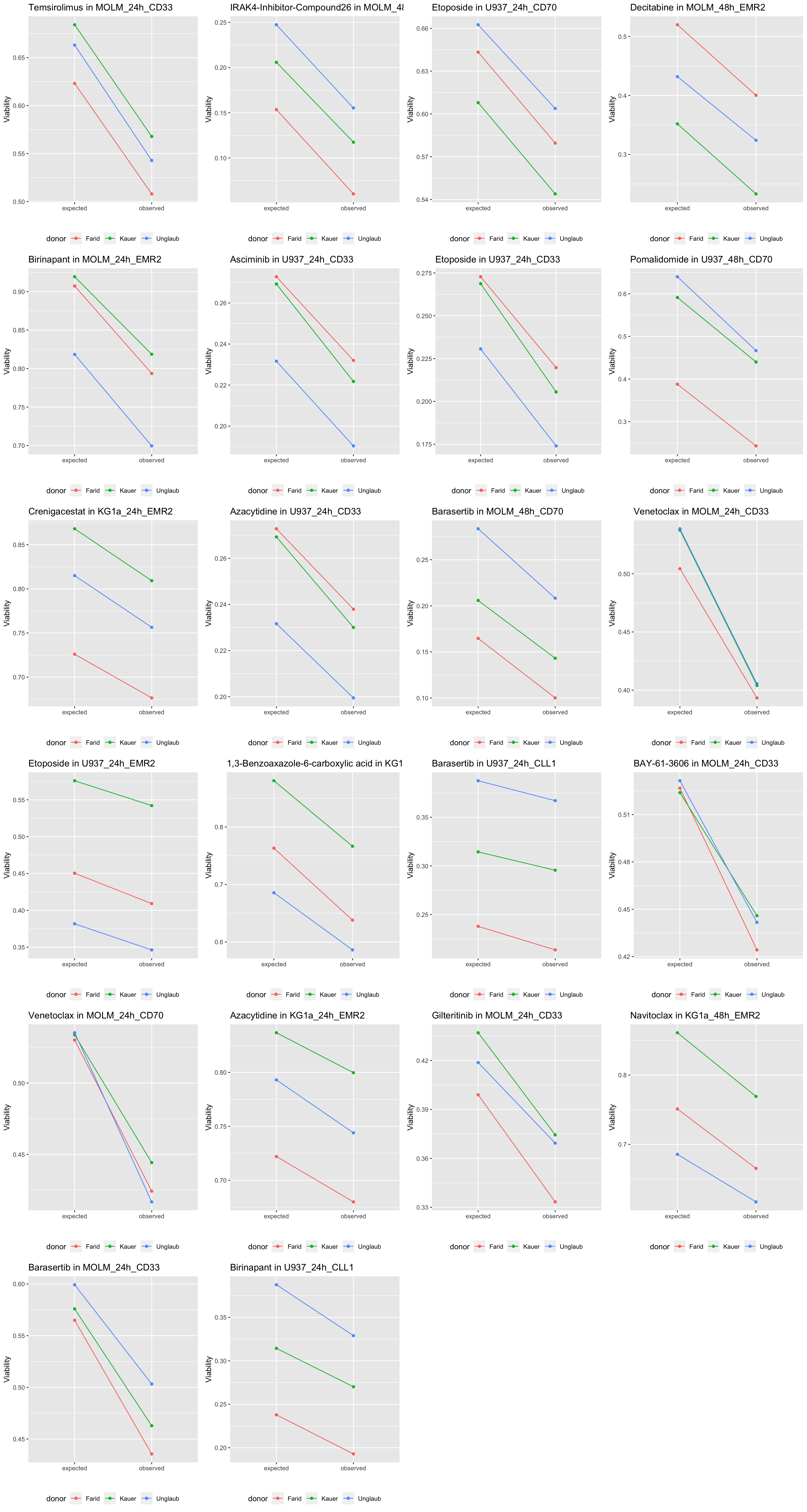
sessionInfo()R version 4.2.0 (2022-04-22)
Platform: x86_64-apple-darwin17.0 (64-bit)
Running under: macOS Big Sur/Monterey 10.16
Matrix products: default
BLAS: /Library/Frameworks/R.framework/Versions/4.2/Resources/lib/libRblas.0.dylib
LAPACK: /Library/Frameworks/R.framework/Versions/4.2/Resources/lib/libRlapack.dylib
locale:
[1] en_US.UTF-8/en_US.UTF-8/en_US.UTF-8/C/en_US.UTF-8/en_US.UTF-8
attached base packages:
[1] stats graphics grDevices utils datasets methods base
other attached packages:
[1] gridExtra_2.3 forcats_0.5.1 stringr_1.4.1 dplyr_1.0.9
[5] purrr_0.3.4 readr_2.1.2 tidyr_1.2.0 tibble_3.1.8
[9] ggplot2_3.4.1 tidyverse_1.3.2 readxl_1.4.0
loaded via a namespace (and not attached):
[1] backports_1.4.1 fastmatch_1.1-3
[3] drc_3.0-1 jyluMisc_0.1.5
[5] workflowr_1.7.0 igraph_1.3.4
[7] shinydashboard_0.7.2 splines_4.2.0
[9] BiocParallel_1.30.3 GenomeInfoDb_1.32.2
[11] TH.data_1.1-1 digest_0.6.30
[13] htmltools_0.5.4 fansi_1.0.3
[15] magrittr_2.0.3 googlesheets4_1.0.0
[17] cluster_2.1.3 tzdb_0.3.0
[19] limma_3.52.2 modelr_0.1.8
[21] matrixStats_0.62.0 sandwich_3.0-2
[23] piano_2.12.0 colorspace_2.0-3
[25] rvest_1.0.2 ggrepel_0.9.1
[27] haven_2.5.0 xfun_0.31
[29] crayon_1.5.2 RCurl_1.98-1.7
[31] jsonlite_1.8.3 survival_3.4-0
[33] zoo_1.8-10 glue_1.6.2
[35] survminer_0.4.9 gtable_0.3.0
[37] gargle_1.2.0 zlibbioc_1.42.0
[39] XVector_0.36.0 DelayedArray_0.22.0
[41] car_3.1-0 BiocGenerics_0.42.0
[43] abind_1.4-5 scales_1.2.0
[45] mvtnorm_1.1-3 DBI_1.1.3
[47] relations_0.6-12 rstatix_0.7.0
[49] Rcpp_1.0.9 plotrix_3.8-2
[51] xtable_1.8-4 km.ci_0.5-6
[53] stats4_4.2.0 DT_0.23
[55] htmlwidgets_1.5.4 httr_1.4.3
[57] fgsea_1.22.0 gplots_3.1.3
[59] ellipsis_0.3.2 pkgconfig_2.0.3
[61] farver_2.1.1 sass_0.4.2
[63] dbplyr_2.2.1 utf8_1.2.2
[65] tidyselect_1.1.2 labeling_0.4.2
[67] rlang_1.0.6 later_1.3.0
[69] visNetwork_2.1.0 munsell_0.5.0
[71] cellranger_1.1.0 tools_4.2.0
[73] cachem_1.0.6 cli_3.4.1
[75] generics_0.1.3 broom_1.0.0
[77] evaluate_0.15 fastmap_1.1.0
[79] yaml_2.3.5 knitr_1.39
[81] fs_1.5.2 survMisc_0.5.6
[83] caTools_1.18.2 mime_0.12
[85] slam_0.1-50 xml2_1.3.3
[87] compiler_4.2.0 rstudioapi_0.13
[89] beeswarm_0.4.0 ggsignif_0.6.3
[91] marray_1.74.0 reprex_2.0.1
[93] bslib_0.4.1 stringi_1.7.8
[95] highr_0.9 lattice_0.20-45
[97] Matrix_1.5-4 KMsurv_0.1-5
[99] shinyjs_2.1.0 vctrs_0.5.2
[101] pillar_1.8.0 lifecycle_1.0.3
[103] jquerylib_0.1.4 data.table_1.14.8
[105] cowplot_1.1.1 bitops_1.0-7
[107] httpuv_1.6.6 GenomicRanges_1.48.0
[109] R6_2.5.1 promises_1.2.0.1
[111] KernSmooth_2.23-20 vipor_0.4.5
[113] IRanges_2.30.0 codetools_0.2-18
[115] MASS_7.3-58 gtools_3.9.3
[117] exactRankTests_0.8-35 assertthat_0.2.1
[119] SummarizedExperiment_1.26.1 rprojroot_2.0.3
[121] withr_2.5.0 multcomp_1.4-19
[123] S4Vectors_0.34.0 GenomeInfoDbData_1.2.8
[125] parallel_4.2.0 hms_1.1.1
[127] grid_4.2.0 rmarkdown_2.14
[129] MatrixGenerics_1.8.1 carData_3.0-5
[131] googledrive_2.0.0 ggpubr_0.4.0
[133] git2r_0.30.1 maxstat_0.7-25
[135] sets_1.0-21 Biobase_2.56.0
[137] shiny_1.7.4 lubridate_1.8.0
[139] ggbeeswarm_0.6.0