Pre-processing and quality control of the AML CART-T drug screen project
Junyan Lu
Last updated: 2023-06-06
Checks: 5 1
Knit directory: combiCART/analysis/
This reproducible R Markdown analysis was created with workflowr (version 1.7.0). The Checks tab describes the reproducibility checks that were applied when the results were created. The Past versions tab lists the development history.
Great job! The global environment was empty. Objects defined in the global environment can affect the analysis in your R Markdown file in unknown ways. For reproduciblity it’s best to always run the code in an empty environment.
The command set.seed(20221110) was run prior to running
the code in the R Markdown file. Setting a seed ensures that any results
that rely on randomness, e.g. subsampling or permutations, are
reproducible.
Great job! Recording the operating system, R version, and package versions is critical for reproducibility.
Nice! There were no cached chunks for this analysis, so you can be confident that you successfully produced the results during this run.
Great job! Using relative paths to the files within your workflowr project makes it easier to run your code on other machines.
Tracking code development and connecting the code version to the
results is critical for reproducibility. To start using Git, open the
Terminal and type git init in your project directory.
This project is not being versioned with Git. To obtain the full
reproducibility benefits of using workflowr, please see
?wflow_start.
Load packages
library(readxl)
library(DrugScreenExplorer)
library(tidyverse)
knitr::opts_chunk$set(warning = FALSE, message = FALSE)
Read screen data
Prepare well annotation file
wellAnno <- readxl::read_excel("../data/wellAnno_AGSauer.xlsx") %>%
  dplyr::rename(Tcell = `Drug_A (T cells)`, Drug = Drug_B, conc = Drug_B.Conc, concStep = Drug_B.ConcStep) %>%
  select(wellID, name, Tcell, Drug, conc, concStep) %>%
  mutate(rowID = str_sub(wellID, 1,2), colID = str_sub(wellID, 3, 4)) %>%
  mutate(ifEdge = rowID %in% c("A0", "P0") | colID %in% c("01","24")) %>% #define only the most outside layer as edge
  select(-rowID, -colID)
Fix some typos in the well annotation file
MI-774,775,776,777 should all be MI-773
wellAnno <- mutate(wellAnno, Drug = ifelse(Drug %in% paste0("MI-", seq(774,777)), "MI-773", Drug))Iburtinib -> Ibrutinib
wellAnno <- mutate(wellAnno, Drug = ifelse(Drug == "Iburtinib", "Ibrutinib", Drug))Save
write_tsv(wellAnno,"../output/wellAnno.tsv")Prepare plate annotation file
smpAnno <- readxl::read_xlsx("../data/plateAnno_AGSauer.xlsx")

plateFile <- list.files("../data/rawData/", recursive = TRUE, pattern = "csv")
plateAnno <- tibble(fileName = plateFile) %>%
  mutate(fileID =basename(fileName)) %>%
  left_join(smpAnno, by = c(fileID = "fileName")) %>%
  select(-fileID) %>%
  dplyr::rename(cellTime = plateID, donorConstruct = Name) %>%
  separate(cellTime, c("cell","time"),"_",remove =FALSE) %>%
  separate(donorConstruct, c("donor","construct"),"_", remove =FALSE) %>%
  mutate(plateID = paste0(cellTime,"_",donorConstruct))

stopifnot(all(!is.na(plateAnno$plateID)))

write_tsv(plateAnno, "../output/plateAnno.tsv")
Read whole screen
without normalization in this step
screenData <- readScreen("../data/rawData/",
                         plateAnnotationFile = "../output/plateAnno.tsv",
                         wellAnnotationFile = "../output/wellAnno.tsv",
                         rowRange = c(7,22), negWell = c("DMSO_Tumor_only"), posWell = c(),
                         colRange = 2, discardLayer = 1, normalization = FALSE, sep = ",")
Perform normalization for different well types
For drug + NT wells, they will be normalized by both NT well
and tumor only wells. For other wells, they will be only normalized by
tumor only wells.
For wells on the edge (most outside layers), they will be
normalized by the tumor only or NT wells on the same layer
Normalize the drug+NT wells by NT only wells
negData <- filter(screenData, name %in% c("DMSO_NT","DMSO_Tumor_only")) %>%
  group_by(plateID, name, ifEdge) %>% summarise(medVal = median(value)) %>%
  mutate(name = ifelse(name == "DMSO_NT", "nt", "dmso")) %>%
  mutate(name = paste0(name, "_", ifelse(ifEdge, "edge","inner"))) %>%
  select(plateID, name, medVal) %>%
  pivot_wider(names_from = name, values_from = medVal)


screenData <- left_join(screenData, negData, by = "plateID") %>%
  mutate(normVal.NT = case_when(!ifEdge & Tcell == "NT" ~ value/nt_inner,
                                !ifEdge & Tcell != "NT" ~ value/dmso_inner,
                                 ifEdge & Tcell == "NT" ~ value/nt_edge,
                                 ifEdge & Tcell != "NT" ~ value/dmso_edge),
         normVal = case_when(!ifEdge ~ value/dmso_inner,
                             ifEdge ~ value/dmso_edge)) %>%
  select(-nt_inner, -nt_edge, -dmso_inner, -dmso_edge)
Quality Control
Plot plate layout
screenData <- screenData %>%
    mutate(type = case_when(
        Drug == "DMSO" & Tcell == "NEG" ~ "control only",
        Drug == "DMSO" & Tcell == "CAR" ~ "CAR only",
        Drug == "DMSO" & Tcell == "NT" ~ "NT only",
        Drug != "DMSO" & Tcell == "CAR" ~ "Drug + CAR",
        Drug != "DMSO" & Tcell == "NT" ~ "Drug + NT"))
The two most outside layer is defined as edges.
Does every plate have the same layout?
plateIden <- group_by(screenData, plateID, wellID) %>%
    summarise(ifSame = length(unique(Drug))==1 &
                  length(unique(Tcell))==1)
all(plateIden$ifSame)
[1] TRUEYes.
Plot drug type layout
plateLayout <- distinct(screenData, rowID, colID, Drug, Tcell, type, concStep)

ggplot(plateLayout, aes(x=colID, y=rowID, fill = type)) +
    geom_tile() +
    theme_classic()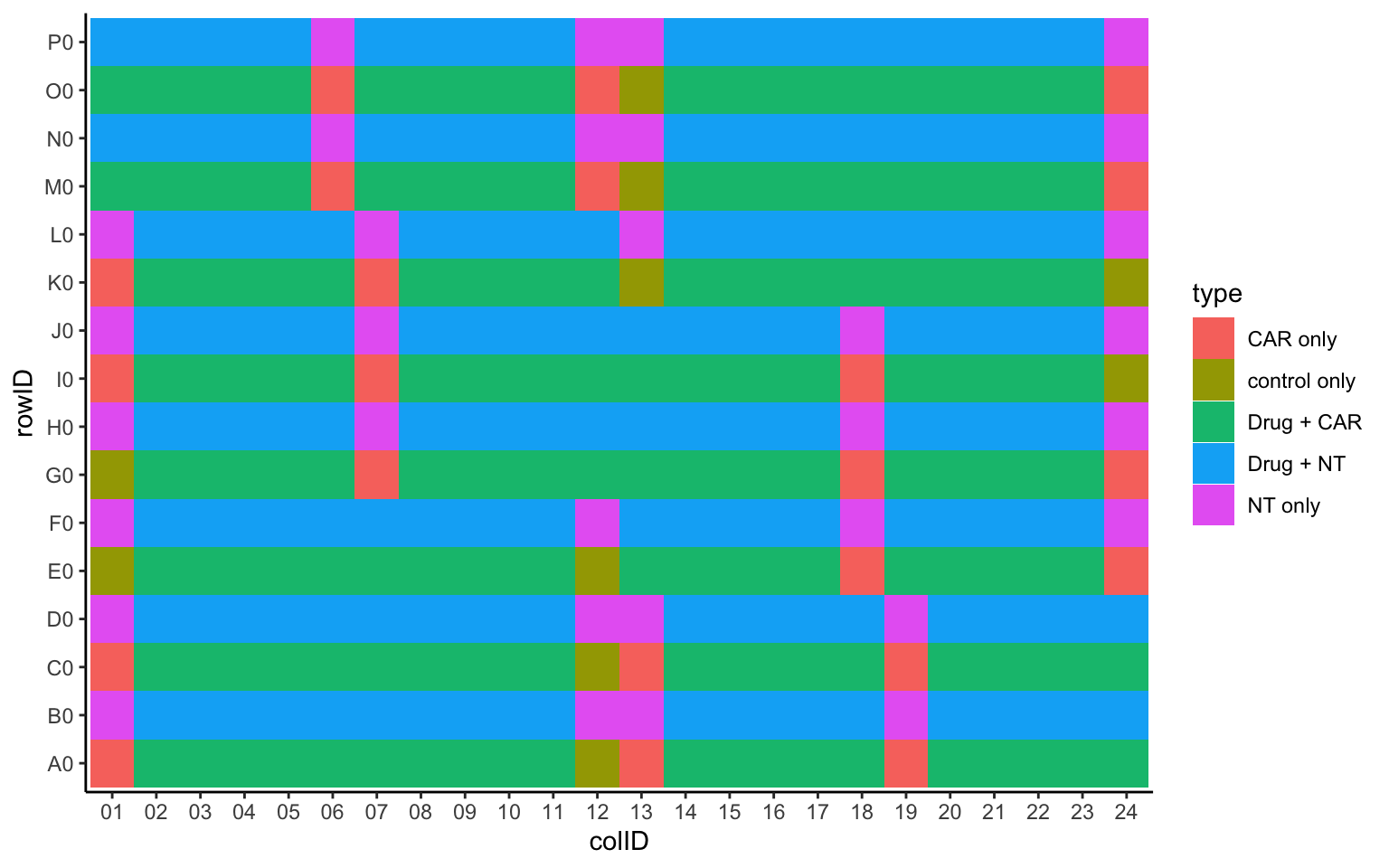
Plot drug layout
ggplot(plateLayout, aes(x=colID, y=rowID, fill = Drug)) +
    geom_tile() +
    theme_classic()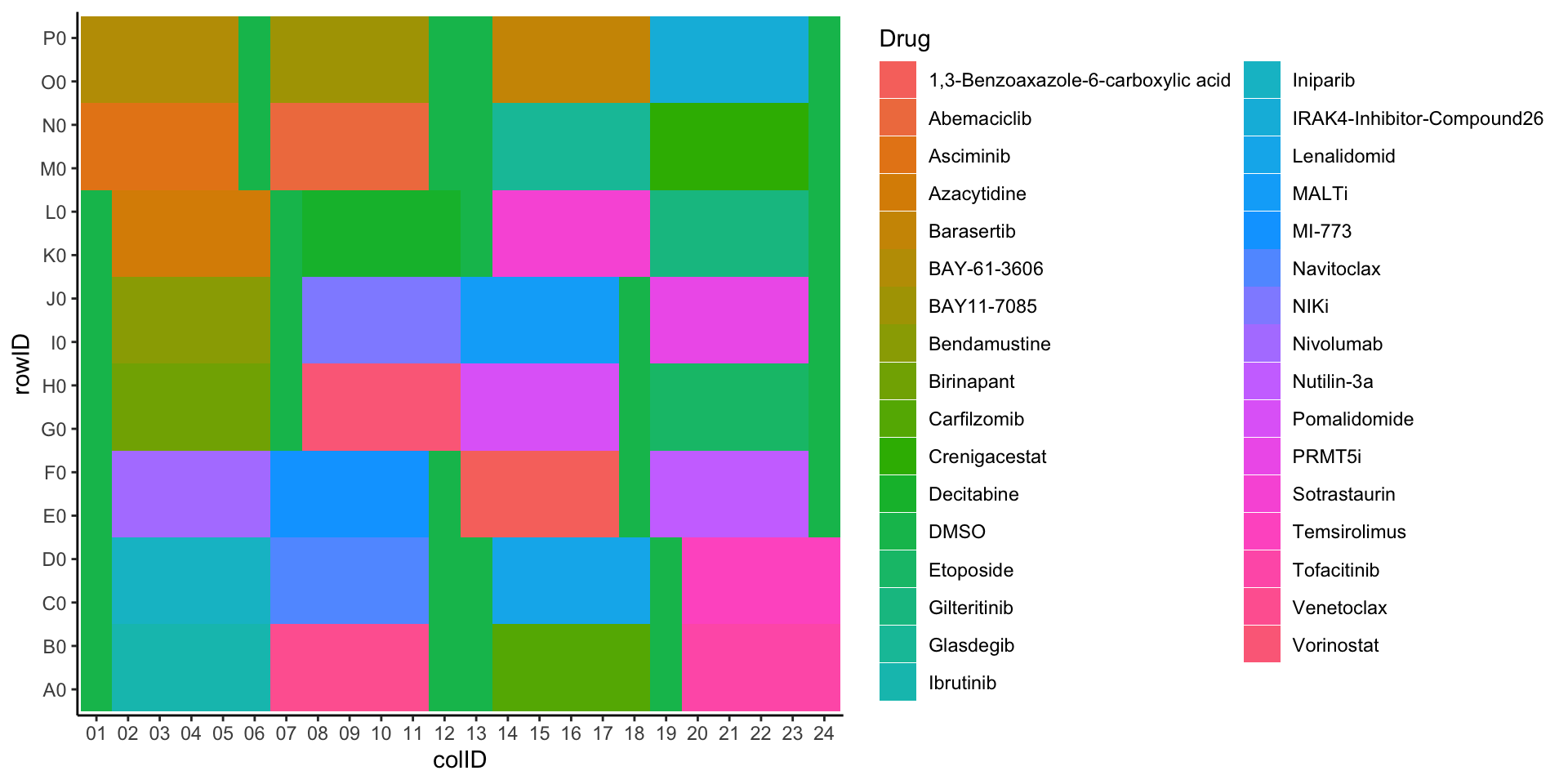
Plot T cell layout
ggplot(plateLayout, aes(x=colID, y=rowID, fill = Tcell)) +
    geom_tile() +
theme_classic() 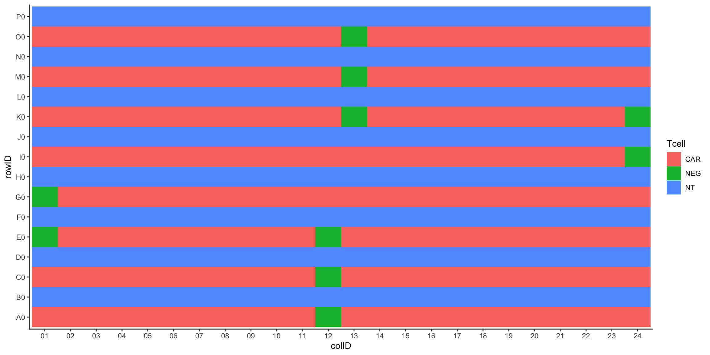
Plot base drug concentration layout
ggplot(plateLayout, aes(x=colID, y=rowID, fill = concStep)) +
    geom_tile() +
theme_classic() 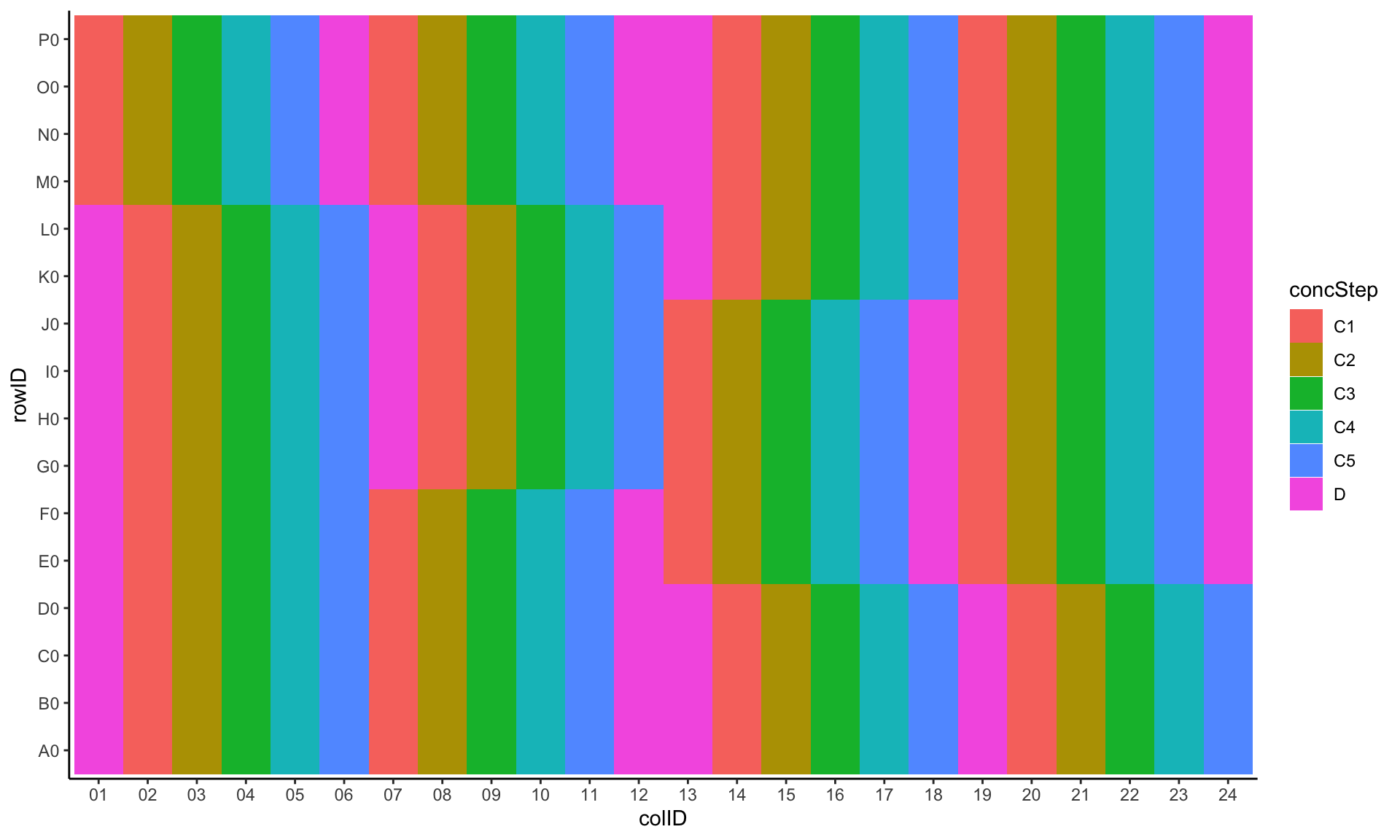
Viability plate plot
pList <- lapply(unique(screenData$plateID), function(id){
    plotTab <- filter(screenData, plateID == id)
    ggplot(plotTab, aes(x=colID, y=rowID, fill = normVal)) +
        geom_tile() +
        scale_fill_gradient2(low = "blue", high = "red", mid = "white", midpoint = 1,limits=c(0,2)) +
        theme_classic() +
        ggtitle(id)
})
jyluMisc::makepdf(pList, "../docs/plate_plot.pdf",ncol = 2, nrow = 3, width = 12, height = 12)Distribution of cell viability in different types of wells
ggplot(screenData, aes(x=type, y=normVal)) +
  geom_violin()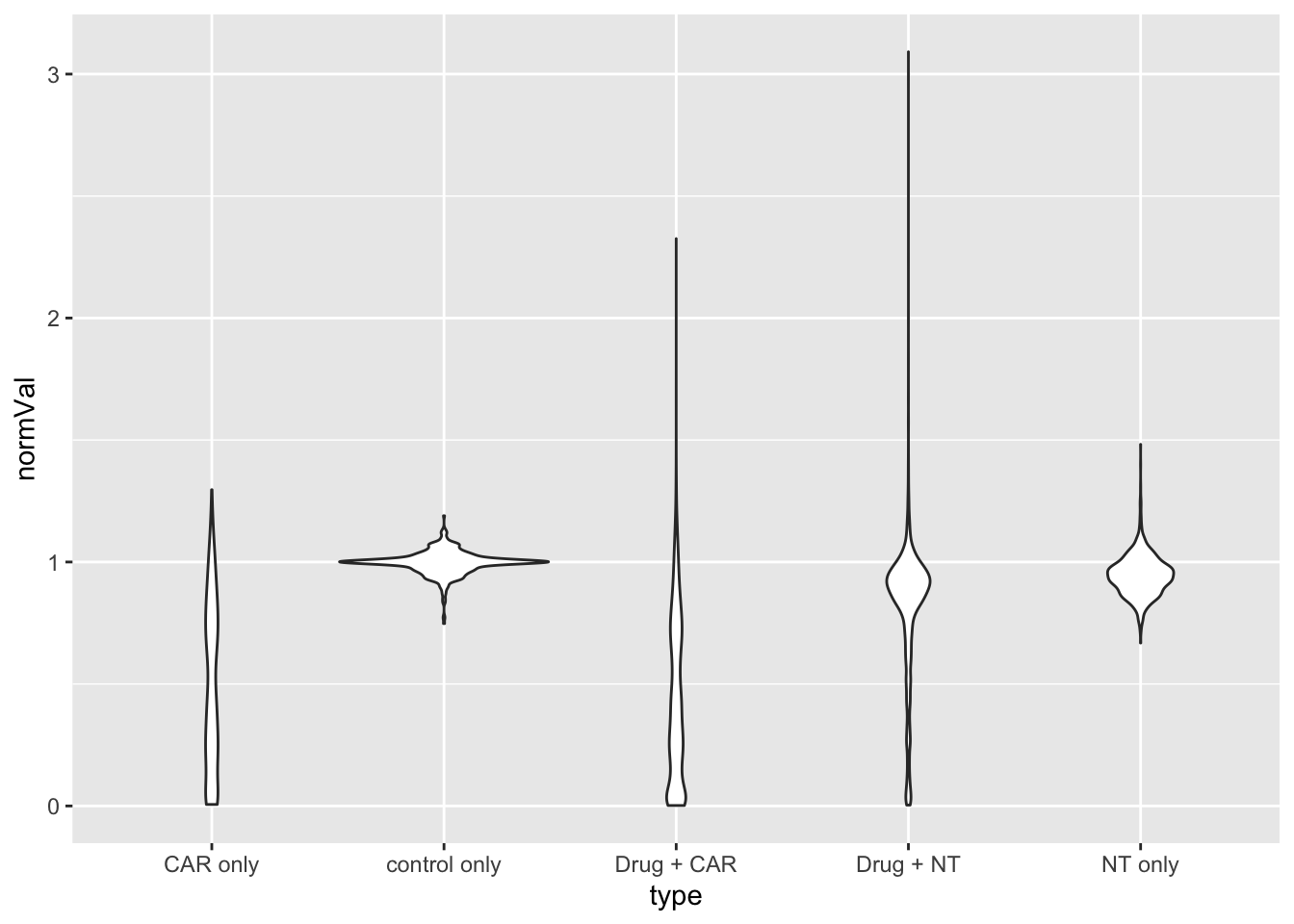
Check control wells
Mean and Variance of internal controls
plotTab <- filter(screenData, type == "control only")
ggplot(plotTab, aes(x=donorConstruct, y=value)) +
    ggbeeswarm::geom_quasirandom(aes(col = ifEdge)) +
    theme(axis.text.x = element_text(angle = 90, vjust=0.5, hjust = 1)) +
  facet_wrap(~cellTime, scale = "free_x")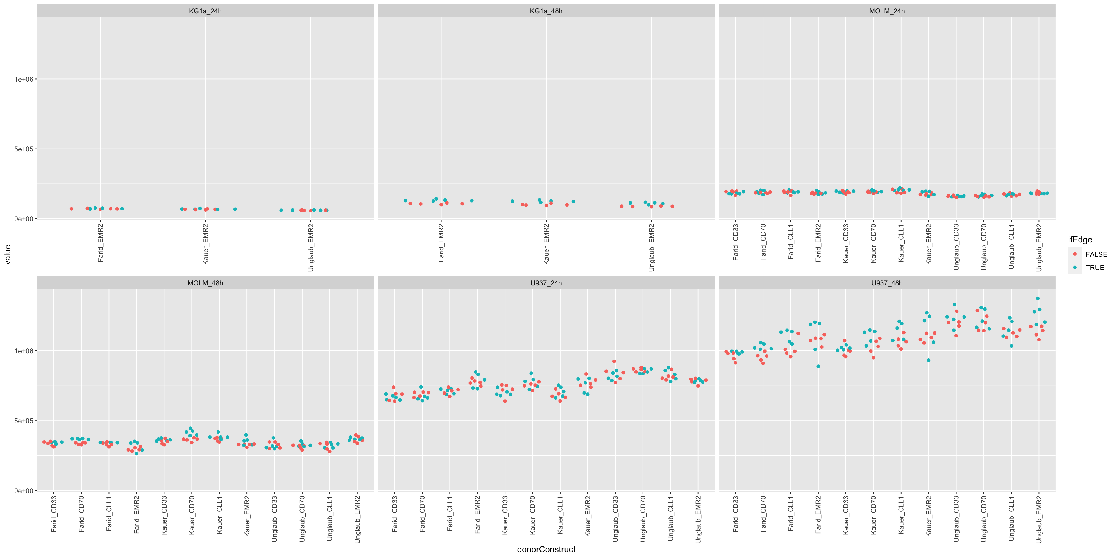
Visualize edge effect
plotTab <- screenData %>% filter(type == "control only")
ggplot(plotTab, aes(x=plateID, y=normVal, col = ifEdge)) +
geom_boxplot() +
theme(axis.text.x = element_text(angle = 90, vjust=0.5, hjust = 1))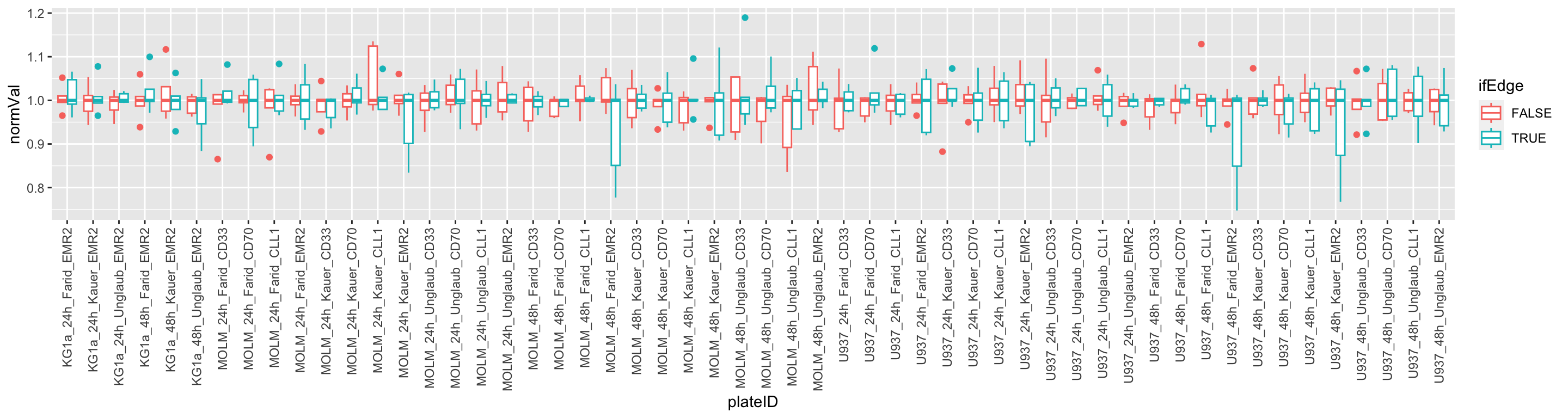 Edge wells seems to have higher variance
Per row
plotTab <- screenData %>% filter(type == "control only")
ggplot(plotTab, aes(x=rowID, y=normVal)) +
geom_boxplot() +
theme(axis.text.x = element_text(angle = 90, vjust=0.5, hjust = 1))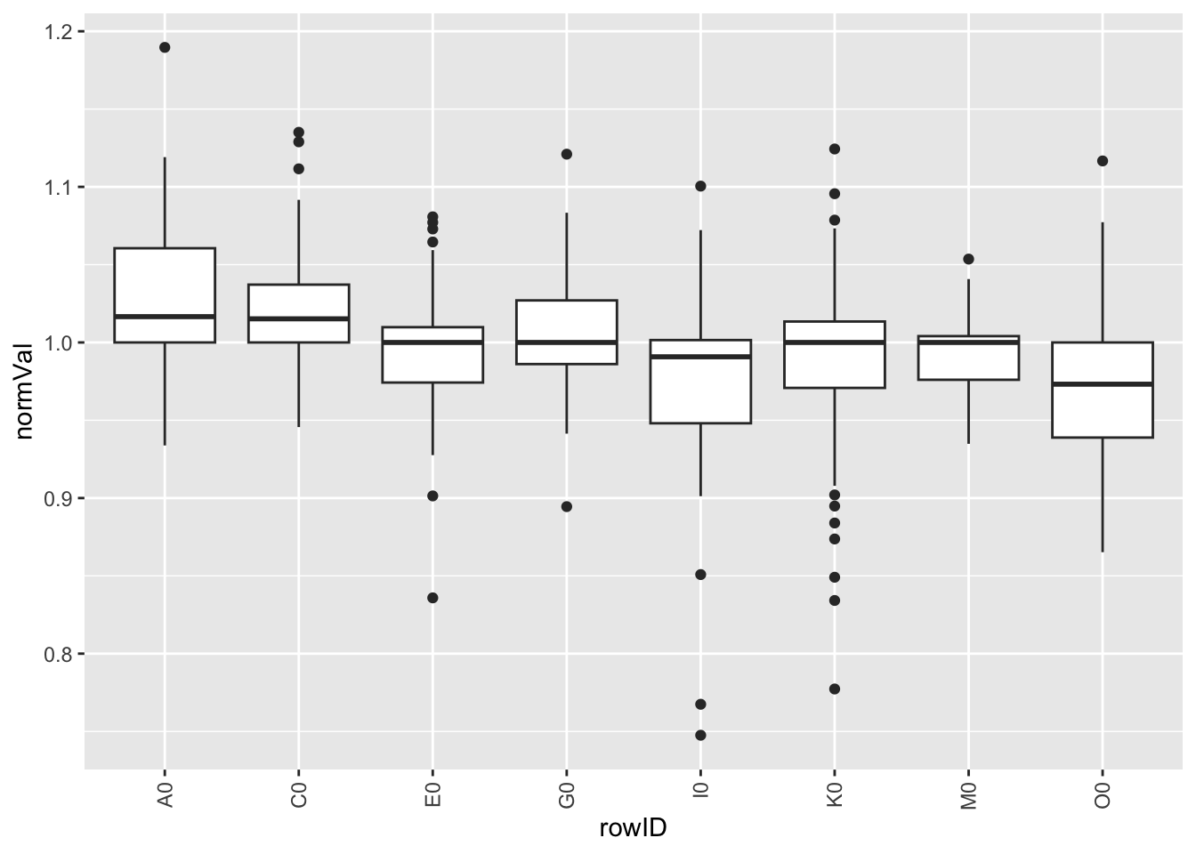 Per column
plotTab <- screenData %>% filter(type == "control only")
ggplot(plotTab, aes(x=colID, y=normVal)) +
geom_boxplot() +
theme(axis.text.x = element_text(angle = 90, vjust=0.5, hjust = 1))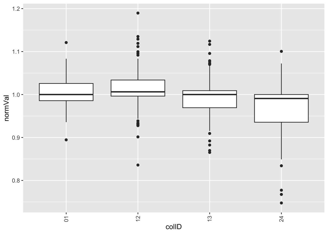 Looks like there’s strong edge effect in this screen.
Visualize Combination design
drugTab <- distinct(screenData, Drug, Tcell, conc) %>%
  mutate(present = 1) %>%
  mutate(drugConc  = paste0(Drug,"_",conc))


orderA <- arrange(drugTab, Drug, conc)$drugConc
orderB <- arrange(drugTab, Tcell)$Tcell

designMat <- drugTab %>%
  select(drugConc, Tcell, present) %>%
  pivot_wider(names_from = Tcell, values_from = present) %>%
  pivot_longer(-drugConc) %>%
  mutate(name = factor(name, levels = unique(orderB)),
         drugConc = factor(drugConc, levels = unique(orderA)))

ggplot(designMat, aes(x=name, y=drugConc, fill = value)) +
  geom_tile() +
  theme_minimal() +
  theme(axis.text.x = element_text(angle = 90, hjust = 1, vjust=0.5))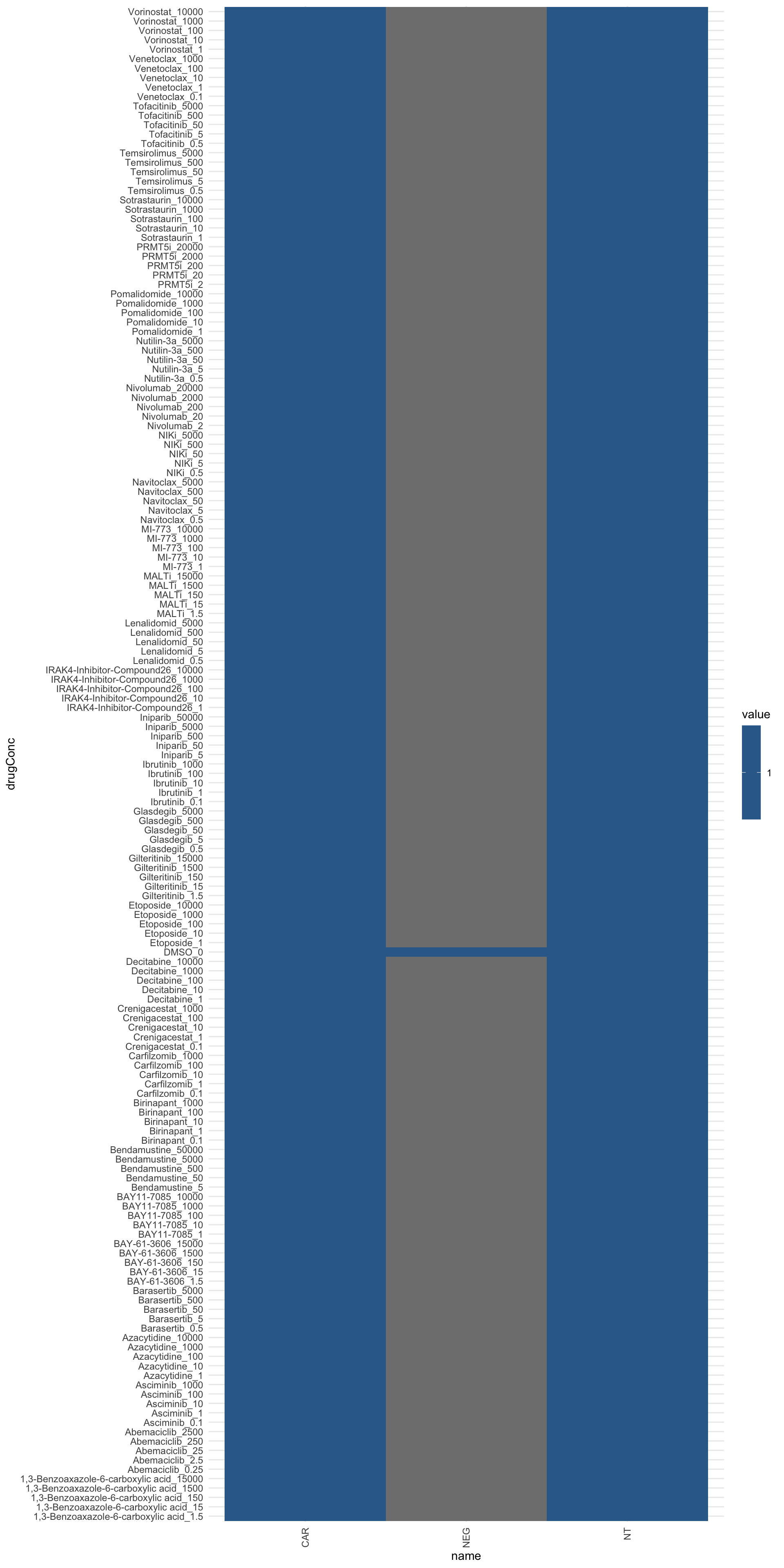
Check if there’s batch effect
Check batch design
table(screenData$screenDate, screenData$cellTime)
             KG1a_24h KG1a_48h MOLM_24h MOLM_48h U937_24h U937_48h
  04.04.2023     1152        0     1152        0     1152        0
  05.04.2023        0     1152        0     1152        0     1152
  07.03.2023        0        0     3456        0     3456        0
  08.03.2023        0        0        0     3456        0     3456
Batch is somewhat confounded with cell lines
Distribution of luminescence signal in different batchs and cell lines
ggplot(screenData, aes(x=screenDate, y=normVal, fill = type)) +
  geom_violin() +
  facet_wrap(~ type, scale = "free", ncol=3) +
  theme(axis.text.x = element_text(angle = 90, hjust = 1, vjust = 0.5))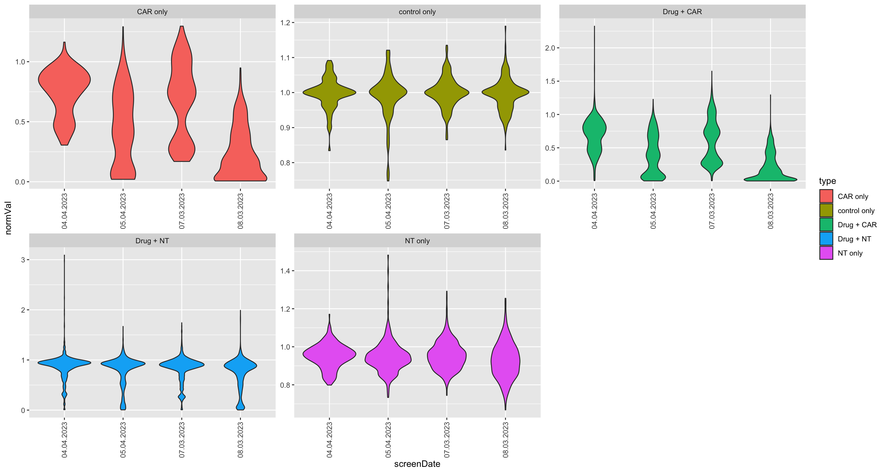
PCA to visualize batch effect
viabMat <- select(screenData, plateID, normVal, wellID) %>%
pivot_wider(names_from = wellID, values_from = normVal) %>%
column_to_rownames("plateID") %>% as.matrix()
pcRes <- prcomp(viabMat)
pcTab <- pcRes$x %>% as_tibble(rownames= "plateID")
varExp <- pcRes$sdev^2/sum(pcRes$sdev^2)
annoTab <- distinct(screenData, plateID, screenDate, cell, time, donor, construct)
plotTab <- left_join(pcTab, annoTab, by = "plateID")
pList <- lapply(seq(6), function(i) {
pc1 <- paste0("PC", 2*(i-1)+1)
pc2 <- paste0("PC", 2*(i-1)+2)
var1 <- varExp[2*(i-1)+1]*100
var2 <- varExp[2*(i-1)+2]*100
ggplot(plotTab, aes_string(x=pc1, y=pc2)) +
geom_point(aes(col = screenDate, size = time, shape = cell)) +
xlab(sprintf("%s (%1.2f%%)", pc1, var1)) +
ylab(sprintf("%s (%1.2f%%)", pc2, var2))
})
cowplot::plot_grid(plotlist = pList, ncol=2)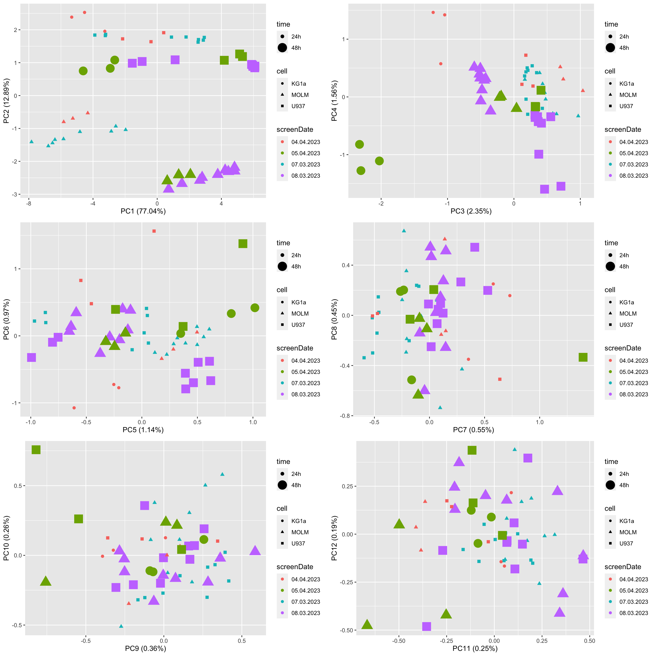 No clear batch effect can be observed.
Save processed data
save(screenData, file = "../output/screenData.RData")
sessionInfo()R version 4.2.0 (2022-04-22)
Platform: x86_64-apple-darwin17.0 (64-bit)
Running under: macOS Big Sur/Monterey 10.16
Matrix products: default
BLAS: /Library/Frameworks/R.framework/Versions/4.2/Resources/lib/libRblas.0.dylib
LAPACK: /Library/Frameworks/R.framework/Versions/4.2/Resources/lib/libRlapack.dylib
locale:
[1] en_US.UTF-8/en_US.UTF-8/en_US.UTF-8/C/en_US.UTF-8/en_US.UTF-8
attached base packages:
[1] stats graphics grDevices utils datasets methods base
other attached packages:
[1] gridExtra_2.3 forcats_0.5.1 stringr_1.4.1
[4] dplyr_1.0.9 purrr_0.3.4 readr_2.1.2
[7] tidyr_1.2.0 tibble_3.1.8 ggplot2_3.4.1
[10] tidyverse_1.3.2 DrugScreenExplorer_0.1.0 readxl_1.4.0
loaded via a namespace (and not attached):
[1] backports_1.4.1 fastmatch_1.1-3
[3] drc_3.0-1 jyluMisc_0.1.5
[5] workflowr_1.7.0 igraph_1.3.4
[7] shinydashboard_0.7.2 splines_4.2.0
[9] BiocParallel_1.30.3 GenomeInfoDb_1.32.2
[11] TH.data_1.1-1 digest_0.6.30
[13] htmltools_0.5.4 fansi_1.0.3
[15] magrittr_2.0.3 tensor_1.5
[17] googlesheets4_1.0.0 cluster_2.1.3
[19] tzdb_0.3.0 limma_3.52.2
[21] modelr_0.1.8 matrixStats_0.62.0
[23] vroom_1.5.7 sandwich_3.0-2
[25] piano_2.12.0 colorspace_2.0-3
[27] rvest_1.0.2 haven_2.5.0
[29] rbibutils_2.2.9 xfun_0.31
[31] crayon_1.5.2 RCurl_1.98-1.7
[33] jsonlite_1.8.3 survival_3.4-0
[35] zoo_1.8-10 glue_1.6.2
[37] survminer_0.4.9 gtable_0.3.0
[39] gargle_1.2.0 zlibbioc_1.42.0
[41] XVector_0.36.0 DelayedArray_0.22.0
[43] car_3.1-0 BiocGenerics_0.42.0
[45] abind_1.4-5 scales_1.2.0
[47] mvtnorm_1.1-3 DBI_1.1.3
[49] relations_0.6-12 rstatix_0.7.0
[51] Rcpp_1.0.9 plotrix_3.8-2
[53] xtable_1.8-4 bit_4.0.4
[55] km.ci_0.5-6 DT_0.23
[57] stats4_4.2.0 htmlwidgets_1.5.4
[59] httr_1.4.3 fgsea_1.22.0
[61] gplots_3.1.3 ellipsis_0.3.2
[63] pkgconfig_2.0.3 farver_2.1.1
[65] sass_0.4.2 dbplyr_2.2.1
[67] utf8_1.2.2 labeling_0.4.2
[69] tidyselect_1.1.2 rlang_1.0.6
[71] later_1.3.0 visNetwork_2.1.0
[73] munsell_0.5.0 cellranger_1.1.0
[75] tools_4.2.0 cachem_1.0.6
[77] cli_3.4.1 generics_0.1.3
[79] broom_1.0.0 evaluate_0.15
[81] fastmap_1.1.0 yaml_2.3.5
[83] knitr_1.39 bit64_4.0.5
[85] fs_1.5.2 survMisc_0.5.6
[87] caTools_1.18.2 mime_0.12
[89] slam_0.1-50 xml2_1.3.3
[91] compiler_4.2.0 rstudioapi_0.13
[93] beeswarm_0.4.0 ggsignif_0.6.3
[95] marray_1.74.0 reprex_2.0.1
[97] bslib_0.4.1 stringi_1.7.8
[99] highr_0.9 lattice_0.20-45
[101] Matrix_1.5-4 KMsurv_0.1-5
[103] shinyjs_2.1.0 vctrs_0.5.2
[105] pillar_1.8.0 lifecycle_1.0.3
[107] Rdpack_2.4 jquerylib_0.1.4
[109] data.table_1.14.8 cowplot_1.1.1
[111] bitops_1.0-7 httpuv_1.6.6
[113] GenomicRanges_1.48.0 R6_2.5.1
[115] promises_1.2.0.1 KernSmooth_2.23-20
[117] vipor_0.4.5 IRanges_2.30.0
[119] codetools_0.2-18 MASS_7.3-58
[121] gtools_3.9.3 exactRankTests_0.8-35
[123] assertthat_0.2.1 SummarizedExperiment_1.26.1
[125] rprojroot_2.0.3 withr_2.5.0
[127] multcomp_1.4-19 S4Vectors_0.34.0
[129] GenomeInfoDbData_1.2.8 parallel_4.2.0
[131] hms_1.1.1 grid_4.2.0
[133] rmarkdown_2.14 MatrixGenerics_1.8.1
[135] carData_3.0-5 dr4pl_2.0.0
[137] googledrive_2.0.0 ggpubr_0.4.0
[139] git2r_0.30.1 maxstat_0.7-25
[141] sets_1.0-21 Biobase_2.56.0
[143] shiny_1.7.4 lubridate_1.8.0
[145] ggbeeswarm_0.6.0