Compare the signature of CHP resistant and sensitive cell lines

workflowr

• Summary
• Checks
• Past versions

Last updated: 2022-08-05

Checks: 5 1

Knit directory: combiDLBCL/analysis/

This reproducible R Markdown analysis was created with workflowr (version 1.7.0). The Checks tab describes the reproducibility checks that were applied when the results were created. The Past versions tab lists the development history.

---

Environment: empty

Great job! The global environment was empty. Objects defined in the global environment can affect the analysis in your R Markdown file in unknown ways. For reproduciblity it’s best to always run the code in an empty environment.

Seed: set.seed(20220425)

The command set.seed(20220425) was run prior to running the code in the R Markdown file. Setting a seed ensures that any results that rely on randomness, e.g. subsampling or permutations, are reproducible.

Session information: recorded

Great job! Recording the operating system, R version, and package versions is critical for reproducibility.

Cache: none

Nice! There were no cached chunks for this analysis, so you can be confident that you successfully produced the results during this run.

File paths: relative

Great job! Using relative paths to the files within your workflowr project makes it easier to run your code on other machines.

Repository version: no version control

Tracking code development and connecting the code version to the results is critical for reproducibility. To start using Git, open the Terminal and type git init in your project directory.

---

This project is not being versioned with Git. To obtain the full reproducibility benefits of using workflowr, please see ?wflow_start.

---

Load libraries and datasets

Data preprocessing

Drug screen data (old CHOP screen data)

load("../data/CHOP_screen_all_data.RData")

CHOP_Screen_data <- CHOP_Screen_data %>%
  mutate(Drug_Conc = as.numeric(Drug_Conc),
         Name = str_replace_all(Name, "_", "-"))

Dose response of CHOP

plotTab <- CHOP_Screen_data 
p <- ggplot(plotTab, aes(x=Drug_Conc, y=Normalized_values, group = Name, col = Name)) +
    geom_line() + geom_point() +
    scale_x_log10() + theme_bw() +
    coord_cartesian(ylim = c(0,1.5)) +
    #ggtitle(paste0(rec$Drug_B)) +
    theme(legend.position = "right") +
    facet_wrap(~drug, scales = "free_x")
p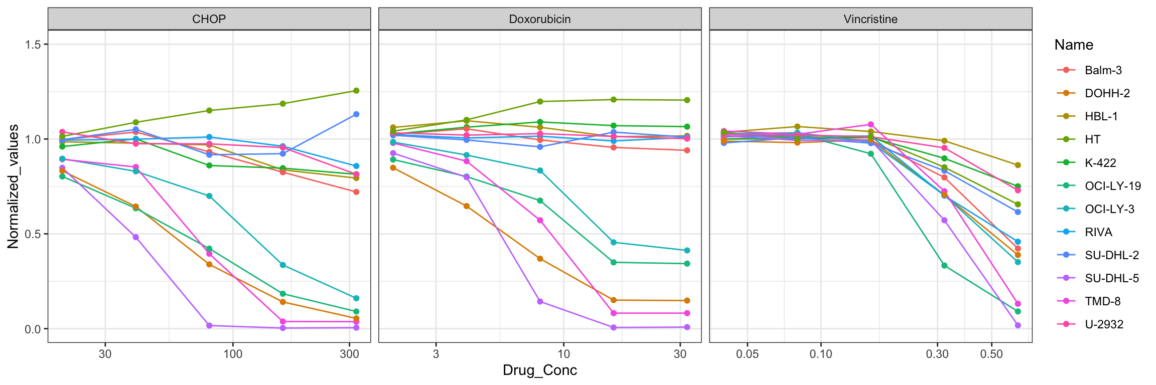

It’s easy to define resistant and sensitive groups

clusterTab <- filter(plotTab, Drug_Conc.Step == "C5", drug == "CHOP") %>%
  mutate(Cluster = ifelse(Normalized_values < 0.5, "sensitive", "resistant")) %>%
  distinct(Name, Cluster) %>%
  mutate(Cluster = factor(Cluster, levels = c("sensitive","resistant"))) %>%
  arrange(Cluster) 
 
clusterTab

# A tibble: 12 × 2
   Name      Cluster  
   <chr>     <fct>    
 1 TMD-8     sensitive
 2 OCI-LY-19 sensitive
 3 OCI-LY-3  sensitive
 4 SU-DHL-5  sensitive
 5 DOHH-2    sensitive
 6 HBL-1     resistant
 7 K-422     resistant
 8 RIVA      resistant
 9 Balm-3    resistant
10 SU-DHL-2  resistant
11 U-2932    resistant
12 HT        resistant

HBL-1 was identified as CHP sensitive (C2) by consensus clustering. HT was identified as C4 group, which shows increased viability by consensus clustering. Others are consistent

Genomics

Processing genomics data

Load genomics

load("../data/SVs_filtered.RData")
svTab <- filter(svTab, Name %in% clusterTab$Name)

Summarise mutations: count as gene mutation if there is at least one mutation within gene

mutTab <- group_by(svTab, Name, Gene) %>% summarise(n = length(Name)) %>%
  arrange(desc(n))

#Get mutations occured at least in three cell lines
geneCount <- group_by(mutTab, Gene) %>% summarise(n=length(Name)) %>%
  filter(n>=3) %>% arrange(desc(n)) %>%
  mutate(Gene = factor(Gene, levels = Gene))

There are too many mutations. Manual curation maybe needed.

Occurrence of mutations among cell lines, only mutations occurred at least 3 times are considered

ggplot(geneCount, aes(x=Gene, y=n)) +
  geom_bar(stat = "identity") +
  theme_bw() + theme(axis.text.x = element_text(angle = 90, hjust = 1, vjust = 0.5))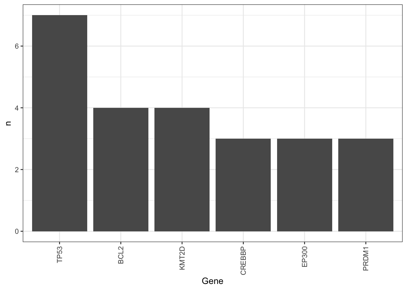

Chi-square test

geneTab <- filter(mutTab, Gene %in% geneCount$Gene) %>%
  mutate(status =1) %>% select(Name, Gene, status) %>%
  pivot_wider(names_from = "Gene", values_from = "status") %>%
  mutate_all(replace_na,0) %>%
  pivot_longer(-Name, names_to = "Gene", values_to = "status") %>%
  ungroup()

testTab <- left_join(geneTab, clusterTab, by = "Name") %>%
  mutate(status = factor(status), Cluster = factor(Cluster))

resTab <- group_by(testTab, Gene) %>% nest() %>%
  mutate(m = map(data, ~chisq.test(.$status,.$Cluster))) %>%
  mutate(res = map(m, broom::tidy)) %>%
  unnest(res) %>%
  select(Gene, p.value)
resTab

# A tibble: 6 × 2
# Groups:   Gene [6]
  Gene   p.value
  <chr>    <dbl>
1 BCL2   0.953  
2 TP53   0.00770
3 EP300  1      
4 KMT2D  1      
5 CREBBP 1      
6 PRDM1  0.565  

TP53 is the most significant one

Dose response of CHOP with TP53 annotated

plotTab <- CHOP_Screen_data %>%
  left_join(filter(geneTab, Gene == "TP53"), by = "Name") %>%
  mutate(annoName = ifelse(Drug_Conc.Step == "C5", Name,""))
p <- ggplot(plotTab, aes(x=Drug_Conc, y=Normalized_values, 
                         group = Name, col = factor(status), label = annoName)) +
    geom_line() + geom_point() +
    scale_x_log10() + theme_bw() +
    coord_cartesian(ylim = c(0,1.5)) +
    ggrepel::geom_text_repel() +
    theme(legend.position = "right") +
    facet_wrap(~drug, scales = "free_x")
p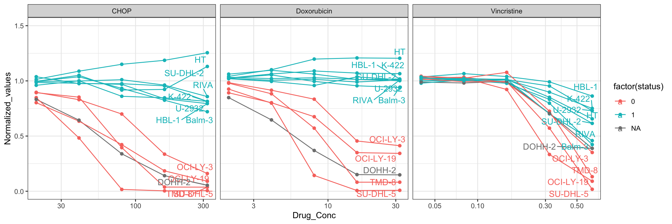

The sensitivity to CHOP is clearly driven by TP53. Based on previous study, DOHH-2 is a TP53 WT cell line (https://www.nature.com/articles/s41598-021-85613-8)

Add TP53 status to the cluster table

clusterTab <- clusterTab %>% 
  left_join(filter(geneTab, Gene == "TP53"), by = "Name") %>%
  mutate(TP53 = case_when(
    Name == "DOHH-2" ~ "WT",
    status == 0 ~ "WT",
    status == 1 ~ "Mut"
  )) %>%
  select(-Gene, -status)

Association with proteomics

Preprocessing proteomic data

Normalization (already performed by Thomas)

protData <- readRDS("../data/SC005_SummarizedExperiment_proteomics.RDS")

#select baseline samples
protData <- protData[, protData$cell.line %in% clusterTab$Name]
protMat <- assay(protData)

#original
boxplot(protMat)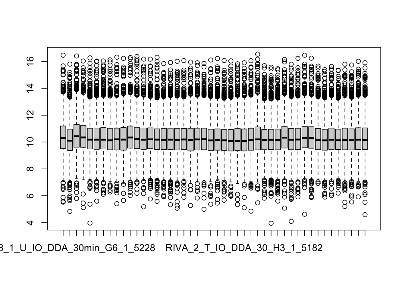

#median normalized
#protMatNorm <- PhosR::medianScaling(protMat, scale = FALSE)
#boxplot(protMatNorm)
protNorm <- protData
#assay(protNorm) <- protMatNorm
assayNames(protNorm) <- "norm"
dim(protNorm)

[1] 2643   46

Average technical replicates for each cell line

protTab <- jyluMisc::sumToTidy(protNorm) %>%
  group_by(cell.line, rowID, Gene_name, condition, Doxo.response) %>%
  summarise(count = mean(norm, na.rm=TRUE)) %>%
  dplyr::rename(symbol = Gene_name, cellLine = cell.line) %>%
  mutate(colID = paste0(cellLine,"_", condition)) %>%
  ungroup()

protAll <- jyluMisc::tidyToSum(protTab, rowID = "rowID", colID = "colID", 
                     values = "count", annoRow = "symbol", 
                     annoCol = c("condition", "cellLine","Doxo.response"))

#add additional annotations
protAll$cluster <- clusterTab[match(protAll$cellLine, clusterTab$Name),]$Cluster
protAll$TP53 <- clusterTab[match(protAll$cellLine, clusterTab$Name),]$TP53

#remove uncessary samples and records
protAll <- protAll[!rowData(protAll)$symbol %in% c("",NA), !is.na(protAll$cluster)]
dim(protAll)

[1] 2641   24

colData(protAll) %>% data.frame() %>% DT::datatable()

SU-DHL-2 should be resistant based on old drug screen, and it’s a TP53 mutated cell line. In the new screen data, SU-DHL-2 sensitivity seems to increased a little, but still between resistant and sensitive.

Differential expression in Baseline (Untreated) condition

protSub <- protAll[,protAll$condition == "U"]

Differential protein expression using proDA

protMat <- assay(protSub)
fit <- proDA(protMat, design = ~ cluster,
             col_data = colData(protSub))

resTab <- test_diff(fit, contrast = "clusterresistant") %>%
  arrange(pval) %>%
  mutate(symbol = rowData(protSub[name,])$symbol)

resTab.base.smart <- resTab #for later comparison with Tobias data

hist(resTab$pval)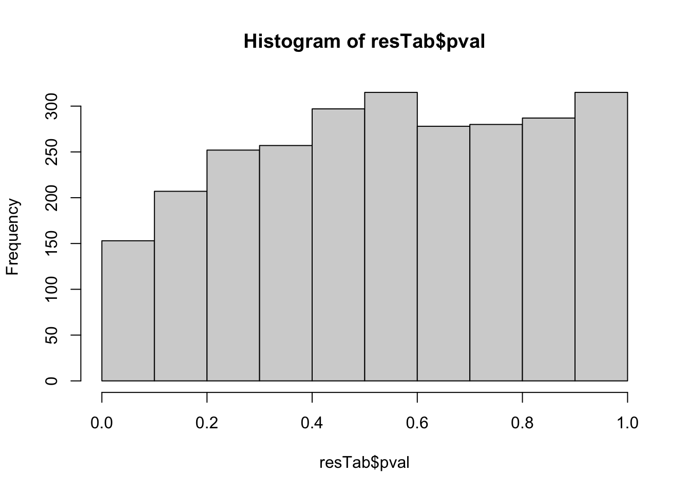

Not strong difference

Proteins with p-value < 0.05

resTab.sig <- filter(resTab, pval < 0.05)
resTab.sig %>% select(symbol, pval, adj_pval, diff) %>%
  mutate_if(is.numeric, formatC, digits=1) %>%
  DT::datatable()

Plot top 9 examples

pList <- lapply(seq(9), function(i) {
  rec <- resTab.sig[i,]
  plotTab <- tibble(expr = protMat[rec$name,],
                    cluster = protSub$cluster,
                    TP53 = protSub$TP53,
                    Name = colnames(protSub)) 
  ggplot(plotTab, aes(x=cluster, y=expr)) +
    geom_boxplot(outlier.shape = NA) +
    ggbeeswarm::geom_quasirandom(aes(color = cluster), size=3) +
    ggrepel::geom_text_repel(aes(label = Name)) +
    ggtitle(rec$symbol) +
    theme_bw() +
    theme(legend.position = "none")
})

cowplot::plot_grid(plotlist = pList,ncol=3)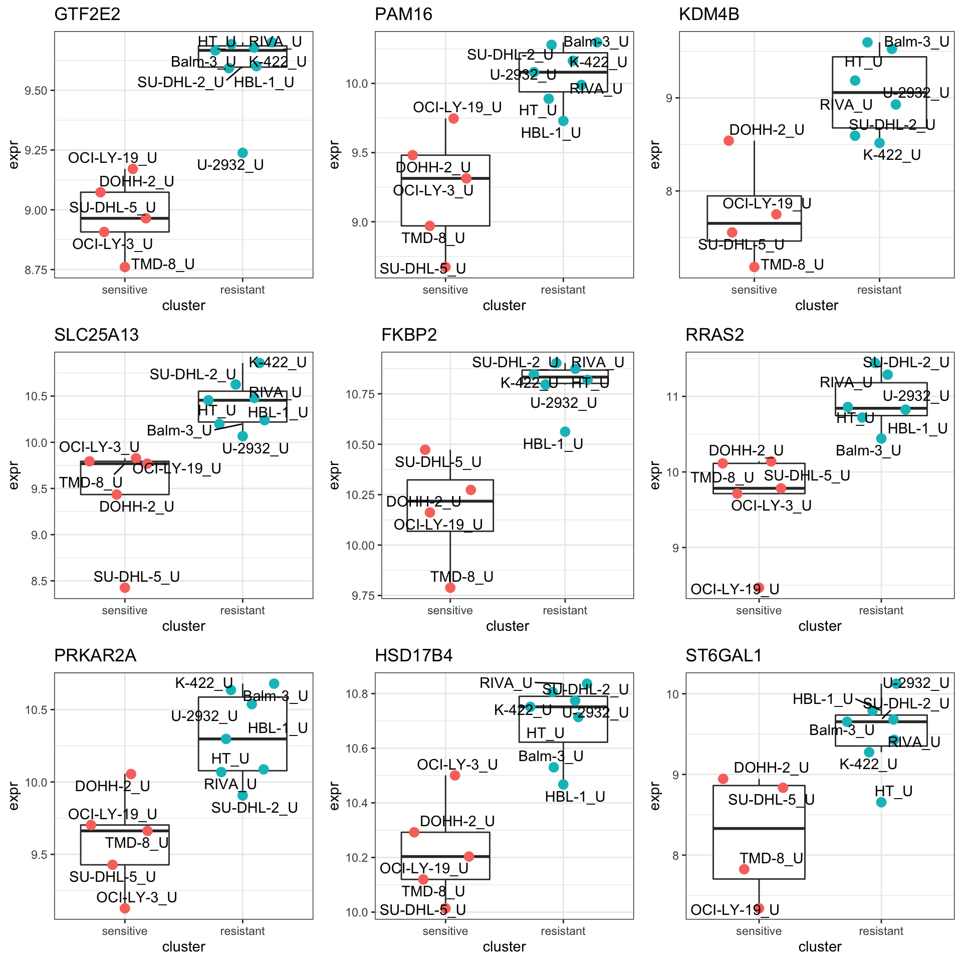

Enrichment analysis

gmts = list(H= "../data/gmts/h.all.v6.2.symbols.gmt",
            KEGG = "../data/gmts/c2.cp.kegg.v6.2.symbols.gmt",
            C6 = "../data/gmts/c6.all.v6.2.symbols.gmt")
inputTab <- resTab %>% filter(pval < 0.1) %>%
  distinct(symbol, .keep_all = TRUE) %>%
  select(symbol, t_statistic) %>% data.frame() %>% column_to_rownames("symbol")
enRes <- list()
enRes[["Hallmark"]] <- runGSEA(inputTab, gmts$H, "page")
enRes[["KEGG"]] <- runGSEA(inputTab, gmts$KEGG,"page")
enRes[["Perturbation"]] <- runGSEA(inputTab, gmts$C6,"page")
p <- plotEnrichmentBar(enRes, pCut =0.05, ifFDR= FALSE)
cowplot::plot_grid(p)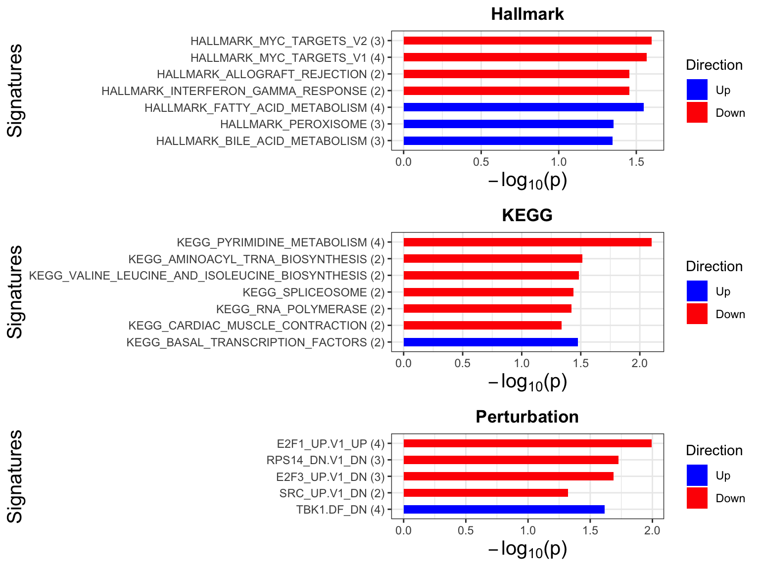

Focus on proteins from Fatty acid metabolism pathway

geneList <- piano::loadGSC(gmts$H)$gsc$HALLMARK_FATTY_ACID_METABOLISM
plotGene <- filter(filter(resTab, pval <= 0.1), symbol%in% geneList )
pList <- lapply(seq(nrow(plotGene)), function(i) {
  rec <- plotGene[i,]
  plotTab <- tibble(expr = protMat[rec$name,],
                    cluster = protSub$cluster,
                    TP53 = protSub$TP53) 
  ggplot(plotTab, aes(x=cluster, y=expr)) +
    geom_boxplot(outlier.shape = NA) +
    ggbeeswarm::geom_quasirandom(aes(color = cluster, shape = TP53), size=3) +
    ggtitle(rec$symbol) +
    theme_bw()
})

cowplot::plot_grid(plotlist = pList,ncol=3)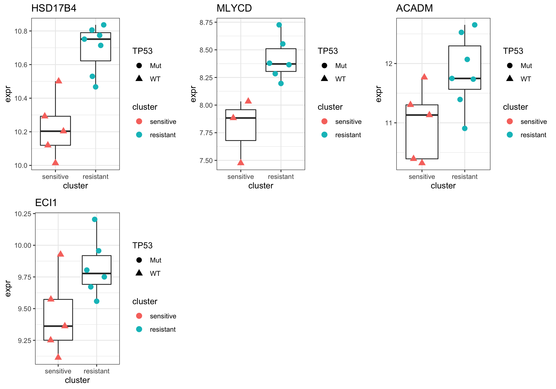

Differential expression in treated (T) condition

protSub <- protAll[,protAll$condition == "T"]

Differential protein expression using proDA

protMat <- assay(protSub)
fit <- proDA(protMat, design = ~ cluster,
             col_data = colData(protSub))

resTab <- test_diff(fit, contrast = "clusterresistant") %>%
  arrange(pval) %>%
  mutate(symbol = rowData(protSub[name,])$symbol)

hist(resTab$pval)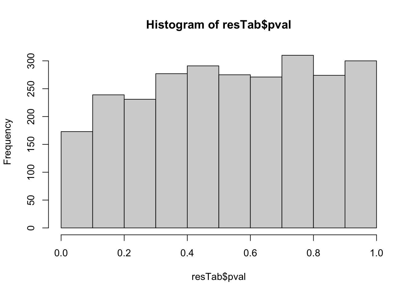

Not strong difference

Proteins with p-value < 0.05

resTab.sig <- filter(resTab, pval < 0.05)
resTab.sig %>% select(symbol, pval, adj_pval, diff) %>%
  mutate_if(is.numeric, formatC, digits=1) %>%
  DT::datatable()

Plot top 9 examples

pList <- lapply(seq(9), function(i) {
  rec <- resTab.sig[i,]
  plotTab <- tibble(expr = protMat[rec$name,],
                    cluster = protSub$cluster,
                    TP53 = protSub$TP53,
                    Name = colnames(protSub)) 
  ggplot(plotTab, aes(x=cluster, y=expr)) +
    geom_boxplot(outlier.shape = NA) +
    ggbeeswarm::geom_quasirandom(aes(color = cluster), size=3) +
    ggrepel::geom_text_repel(aes(label = Name)) +
    ggtitle(rec$symbol) +
    theme_bw()+
    theme(legend.position = "none")
})

cowplot::plot_grid(plotlist = pList,ncol=3)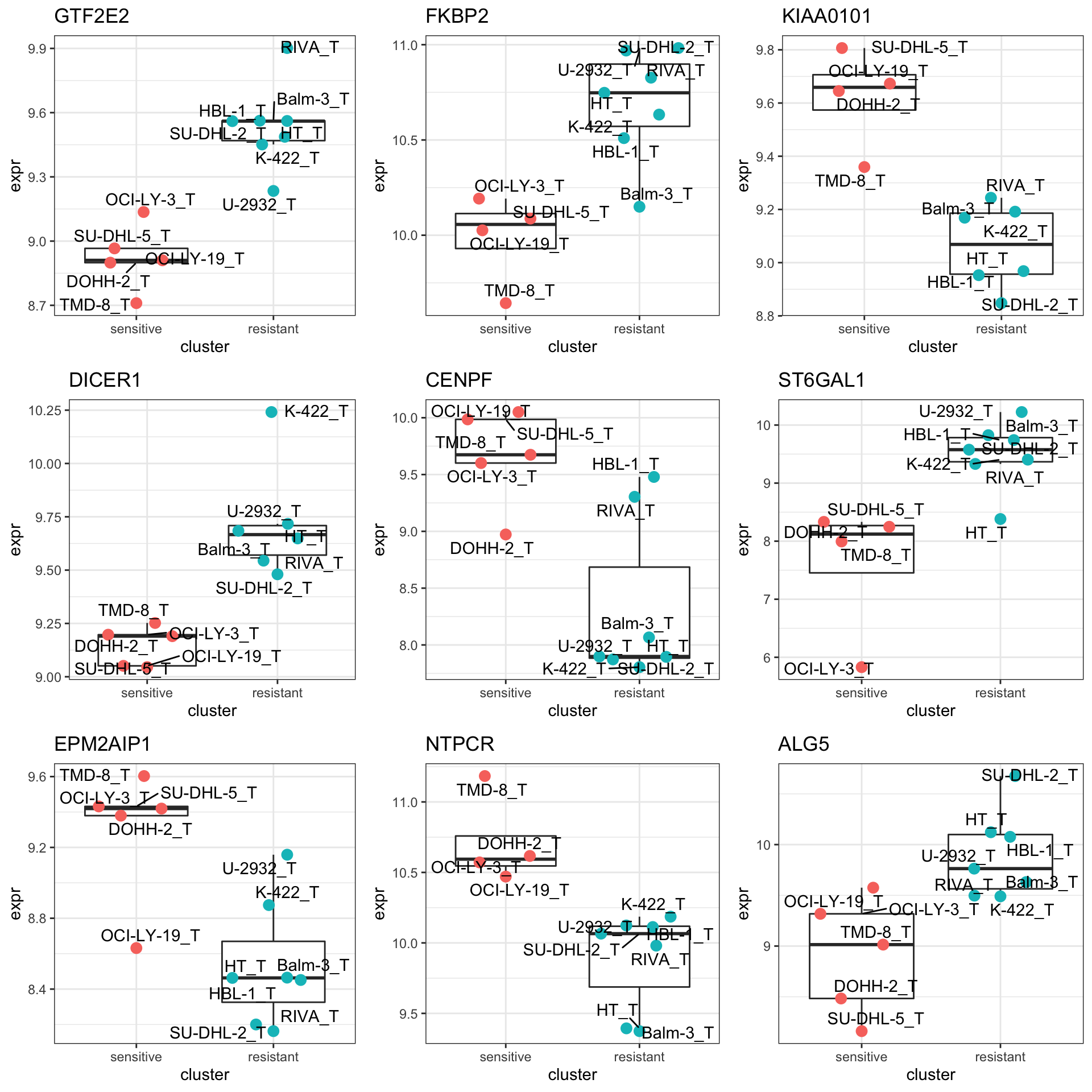

Enrichment analysis

gmts = list(H= "../data/gmts/h.all.v6.2.symbols.gmt",
            KEGG = "../data/gmts/c2.cp.kegg.v6.2.symbols.gmt",
            C6 = "../data/gmts/c6.all.v6.2.symbols.gmt")
inputTab <- resTab %>% filter(pval < 0.1) %>%
  distinct(symbol, .keep_all = TRUE) %>%
  select(symbol, t_statistic) %>% data.frame() %>% column_to_rownames("symbol")
enRes <- list()
enRes[["Hallmark"]] <- runGSEA(inputTab, gmts$H, "page")
enRes[["KEGG"]] <- runGSEA(inputTab, gmts$KEGG,"page")
enRes[["Perturbation"]] <- runGSEA(inputTab, gmts$C6,"page")
p <- plotEnrichmentBar(enRes, pCut =0.05, ifFDR= FALSE)
cowplot::plot_grid(p)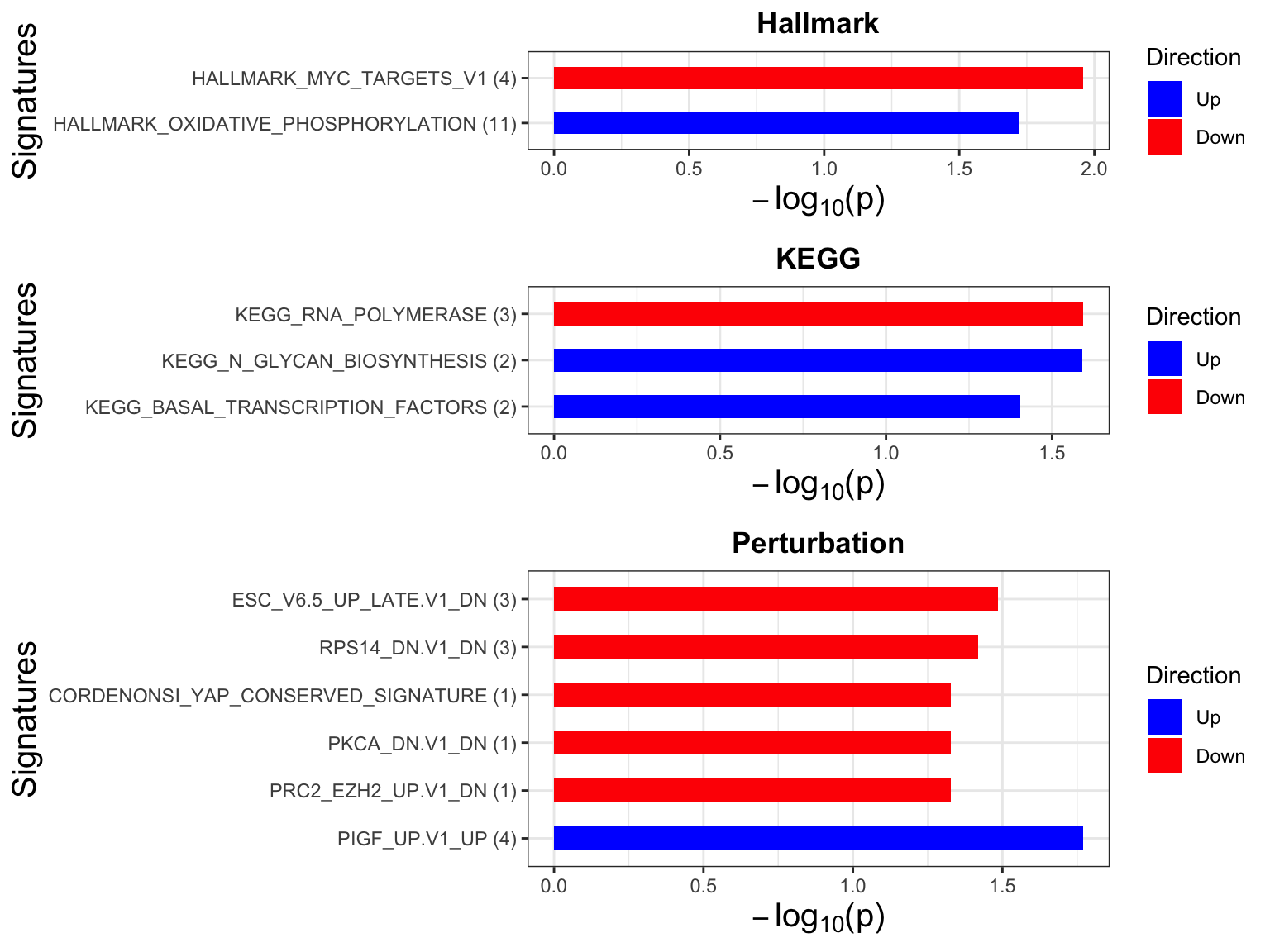

Focus on proteins from Fatty acid metabolism pathway

geneList <- piano::loadGSC(gmts$H)$gsc$HALLMARK_FATTY_ACID_METABOLISM
plotGene <- filter(filter(resTab, pval <= 0.1), symbol%in% geneList )
pList <- lapply(seq(nrow(plotGene)), function(i) {
  rec <- plotGene[i,]
  plotTab <- tibble(expr = protMat[rec$name,],
                    cluster = protSub$cluster,
                    TP53 = protSub$TP53) 
  ggplot(plotTab, aes(x=cluster, y=expr)) +
    geom_boxplot(outlier.shape = NA) +
    ggbeeswarm::geom_quasirandom(aes(color = cluster, shape = TP53), size=3) +
    ggtitle(rec$symbol) +
    theme_bw()
})

cowplot::plot_grid(plotlist = pList,ncol=3)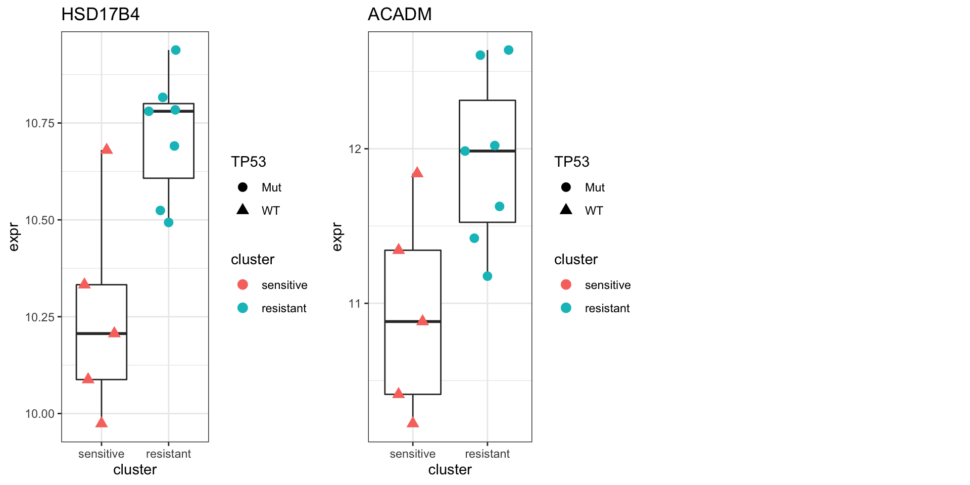

Differential expression between treated and untreated

protSub <- protAll

Differential protein expression using proDA

protMat <- assay(protSub)
fit <- proDA(protMat, design = ~ cellLine + condition,
             col_data = colData(protSub))

resTab <- test_diff(fit, contrast = "conditionT") %>%
  arrange(pval) %>%
  mutate(symbol = rowData(protSub[name,])$symbol)

hist(resTab$pval)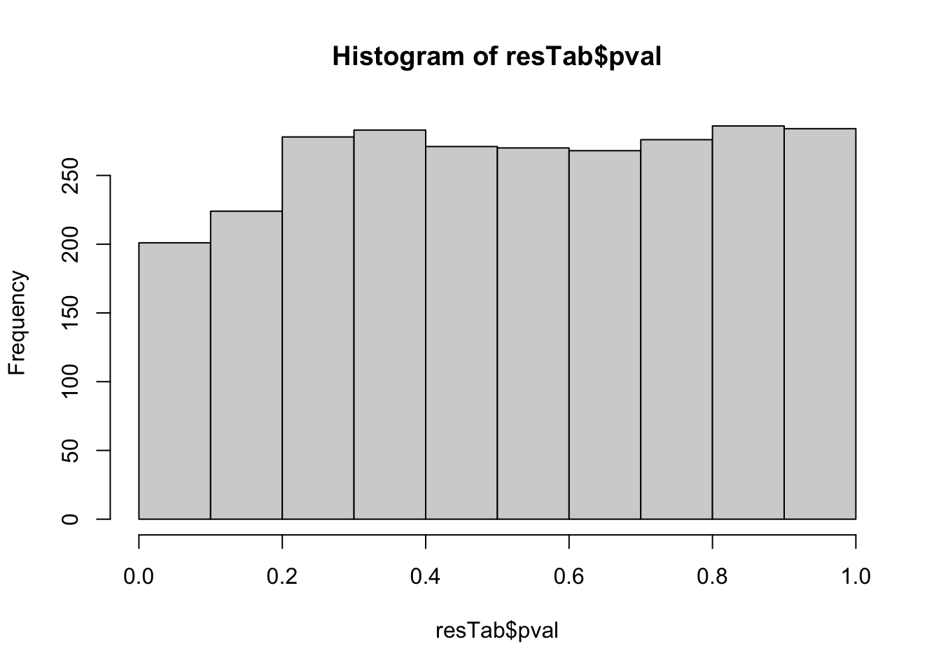

Not strong difference

Proteins with p-value < 0.05

resTab.sig <- filter(resTab, pval < 0.05)
resTab.sig %>% select(symbol, pval, adj_pval, diff) %>%
  mutate_if(is.numeric, formatC, digits=1) %>%
  DT::datatable()

Plot top 9 examples

pList <- lapply(seq(9), function(i) {
  rec <- resTab.sig[i,]
  plotTab <- tibble(expr = protMat[rec$name,],
                    cluster = protSub$cluster,
                    Name = protSub$cellLine,
                    condition = protSub$condition) 
  ggplot(plotTab, aes(x=condition, y=expr)) +
    geom_boxplot(outlier.shape = NA) +
    geom_point(aes(color = cluster), size=3) +
    geom_line(aes(group = Name), linetype = "dotted") +
    ggrepel::geom_text_repel(aes(label = Name)) +
    ggtitle(rec$symbol) +
    theme_bw()
})

cowplot::plot_grid(plotlist = pList,ncol=3)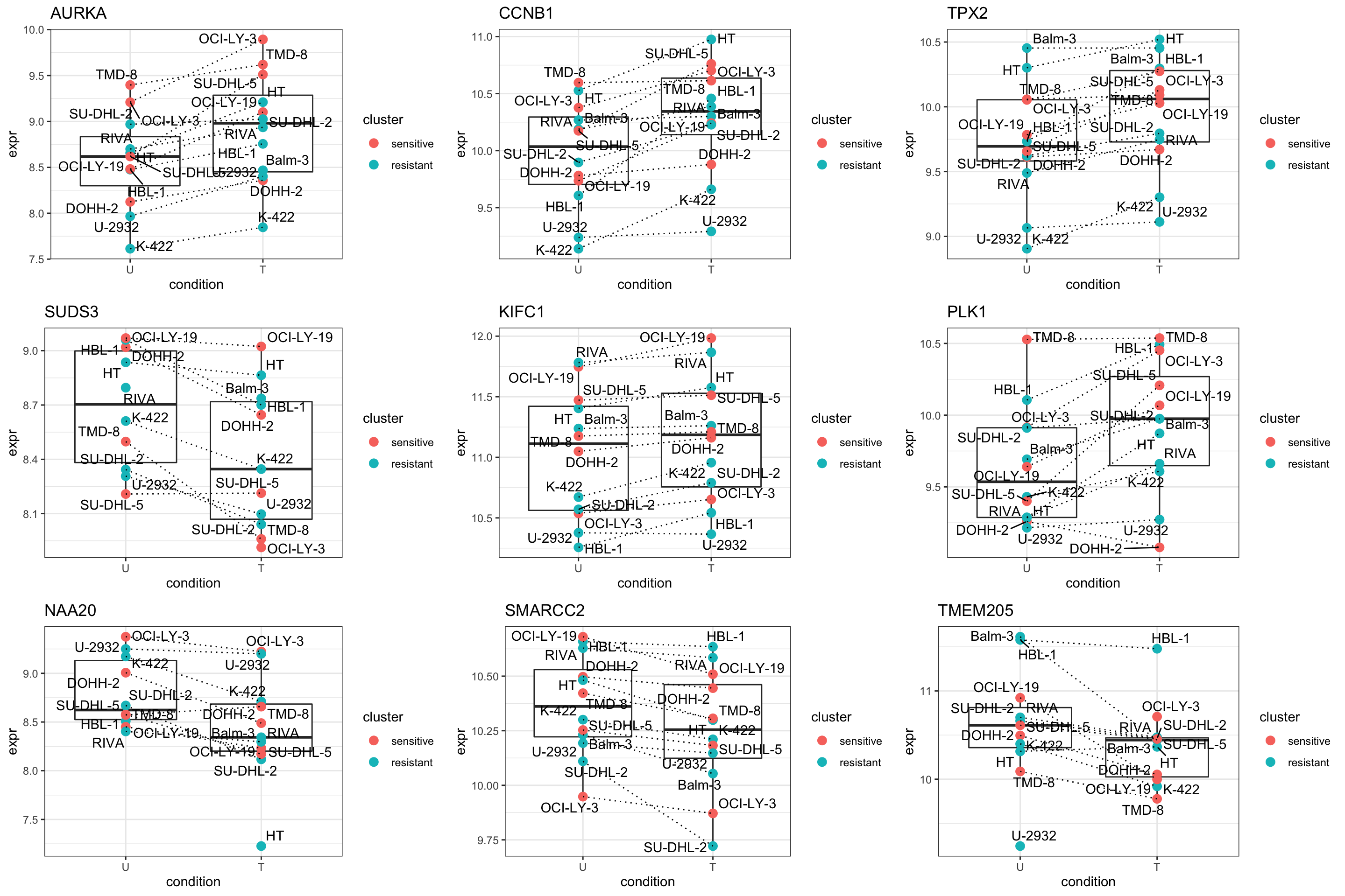

Enrichment analysis

gmts = list(H= "../data/gmts/h.all.v6.2.symbols.gmt",
            KEGG = "../data/gmts/c2.cp.kegg.v6.2.symbols.gmt",
            C6 = "../data/gmts/c6.all.v6.2.symbols.gmt")
inputTab <- resTab %>% filter(pval < 0.1) %>%
  distinct(symbol, .keep_all = TRUE) %>%
  select(symbol, t_statistic) %>% data.frame() %>% column_to_rownames("symbol")
enRes <- list()
enRes[["Hallmark"]] <- runGSEA(inputTab, gmts$H, "page")
enRes[["KEGG"]] <- runGSEA(inputTab, gmts$KEGG,"page")
enRes[["Perturbation"]] <- runGSEA(inputTab, gmts$C6,"page")
p <- plotEnrichmentBar(enRes, pCut =0.05, ifFDR= FALSE)
cowplot::plot_grid(p)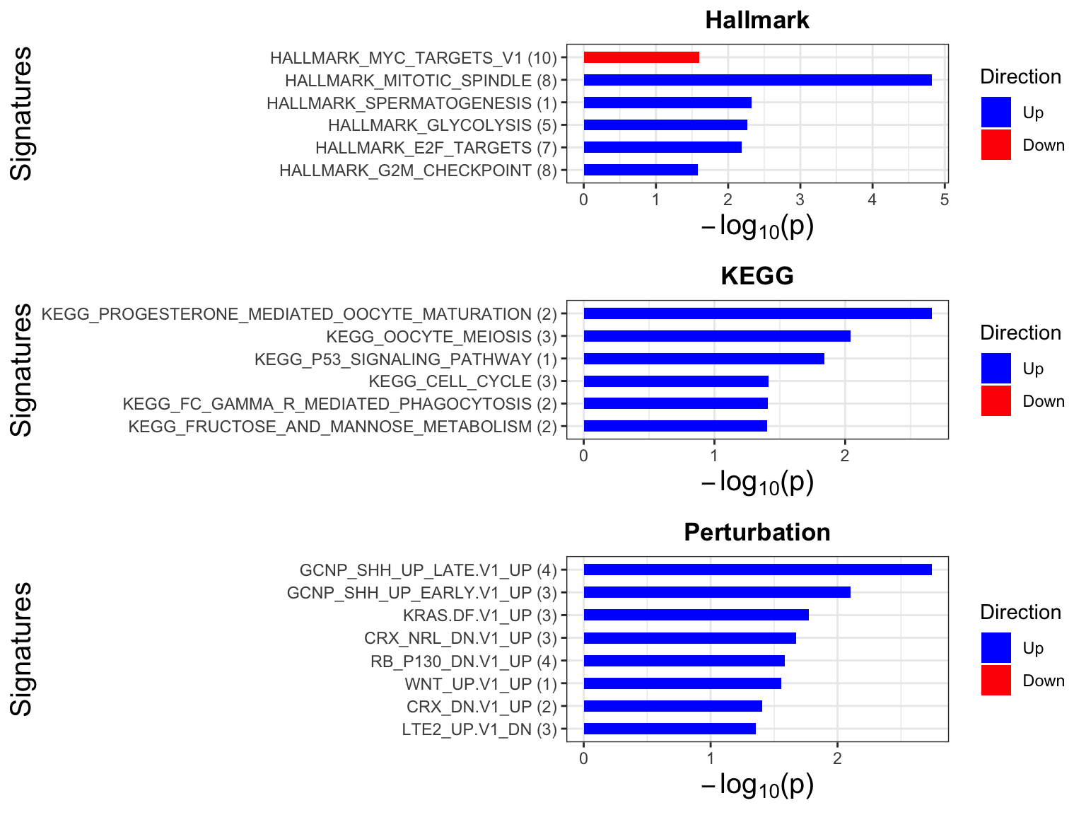

Interaction between treatment and sensitivity cluster

protSub <- protAll

Differential protein expression using proDA

protMat <- assay(protSub)
design <- model.matrix(~ 0 + condition*cluster, data = colData(protSub)) 
colnames(design) <- make.names(colnames(design))

cor <- duplicateCorrelation(protMat, design, block=protSub$cellLine)
#cor$consensus.correlation

fit <- lmFit(object=protMat, design=design, block=protSub$cellLine,
    correlation = cor$consensus.correlation, method = "ls")
fit2 <- eBayes(fit)
resTab  <- topTable(fit2, number = Inf, coef="conditionT.clusterresistant") %>%
  as_tibble(rownames = "name") %>%
  mutate(symbol = rowData(protSub[name,])$symbol) %>%
  dplyr::rename(pval = P.Value, adj_pval = adj.P.Val, diff = logFC, t_statistics = t)

hist(resTab$pval)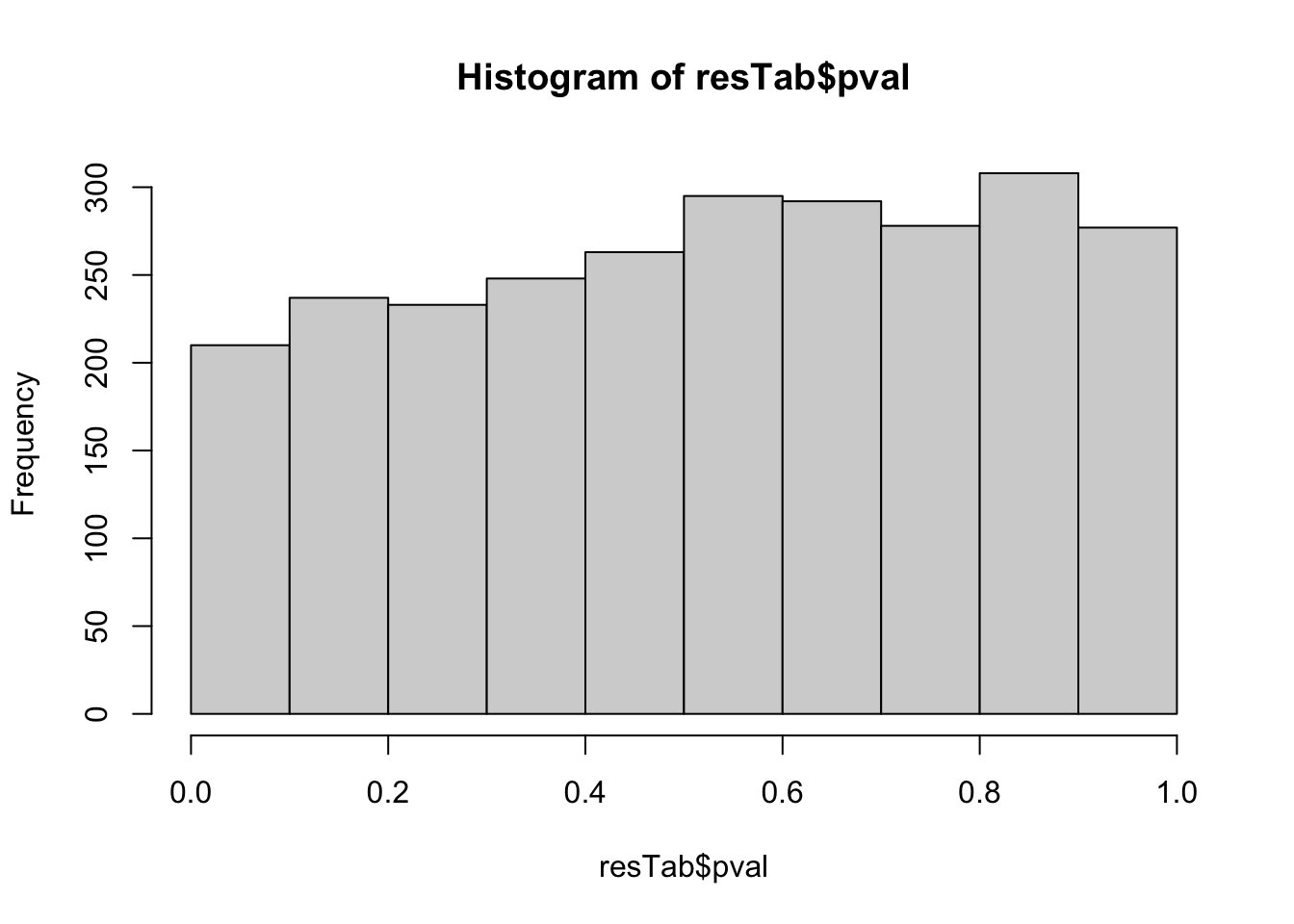

Not strong difference

Proteins with p-value < 0.05

resTab.sig <- filter(resTab, pval < 0.05)
resTab.sig %>% select(symbol, pval, adj_pval, diff) %>%
  mutate_if(is.numeric, formatC, digits=1) %>%
  DT::datatable()

Plot top 9 examples

pList <- lapply(seq(9), function(i) {
  rec <- resTab.sig[i,]
  plotTab <- tibble(expr = protMat[rec$name,],
                    cluster = protSub$cluster,
                    Name = protSub$cellLine,
                    condition = protSub$condition) 
  ggplot(plotTab, aes(x=condition, y=expr)) +
    geom_boxplot(outlier.shape = NA) +
    geom_point(aes(color = cluster), size=3) +
    geom_line(aes(group = Name), linetype = "dotted") +
    ggrepel::geom_text_repel(aes(label = Name)) +
    ggtitle(rec$symbol) +
    theme_bw() +
    facet_wrap(~cluster)
})

cowplot::plot_grid(plotlist = pList,ncol=3)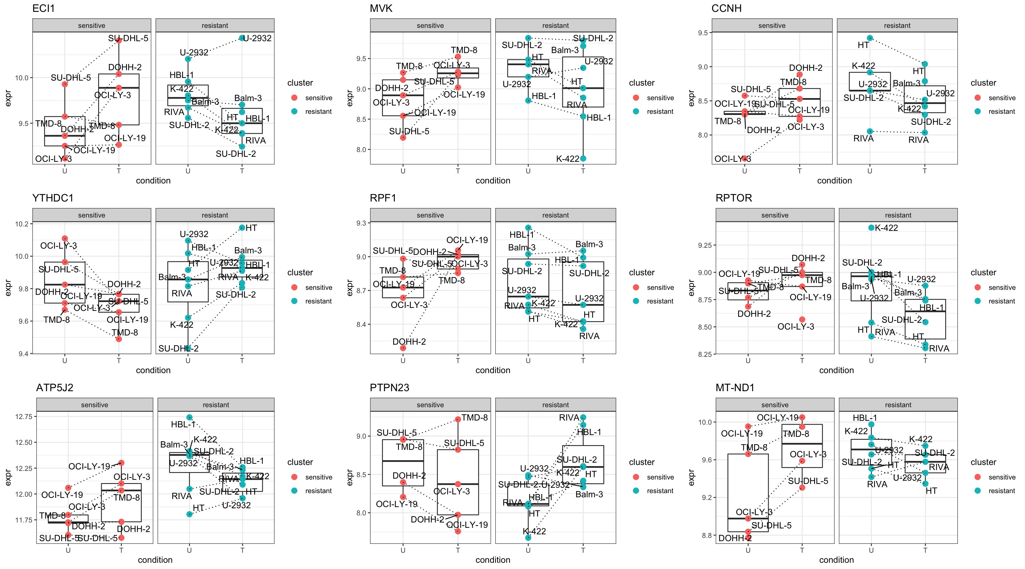

Enrichment analysis

gmts = list(H= "../data/gmts/h.all.v6.2.symbols.gmt",
            KEGG = "../data/gmts/c2.cp.kegg.v6.2.symbols.gmt",
            C6 = "../data/gmts/c6.all.v6.2.symbols.gmt")
inputTab <- resTab %>% filter(pval < 0.1) %>%
  distinct(symbol, .keep_all = TRUE) %>%
  select(symbol, t_statistics) %>% data.frame() %>% column_to_rownames("symbol")
enRes <- list()

enRes[["Hallmark"]] <- runGSEA(inputTab, gmts$H, "page")
enRes[["KEGG"]] <- runGSEA(inputTab, gmts$KEGG,"page")
enRes[["Perturbation"]] <- runGSEA(inputTab, gmts$C6,"page")
p <- plotEnrichmentBar(enRes, pCut =0.05, ifFDR= FALSE)
cowplot::plot_grid(p)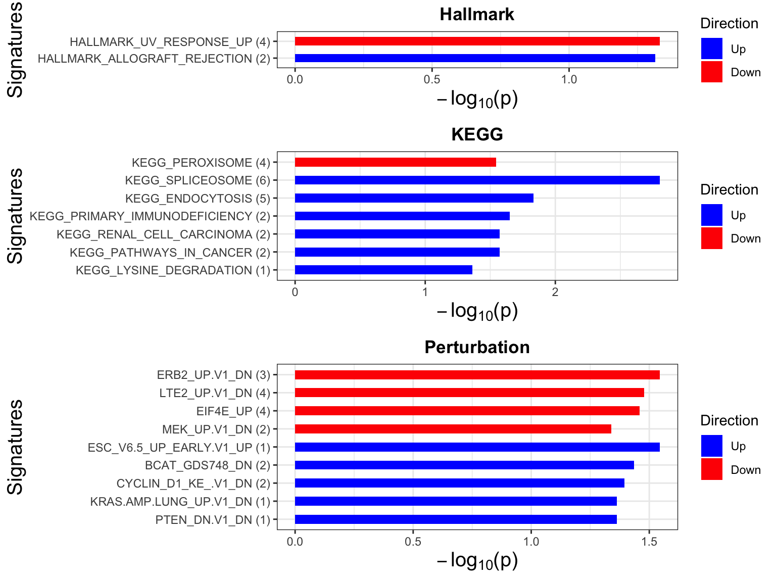

Baseline proteomics dataset from Tobias (EMBL dataset)

Data distribution

load("../data/ProtWide.RData")
ProtWide <- ProtWide[,colnames(ProtWide) %in% clusterTab$Name]
protMat <- ProtWide
dim(ProtWide)

[1] 4873   12

Median normalization (not performed)

protMatNorm <- protMat
boxplot(protMatNorm)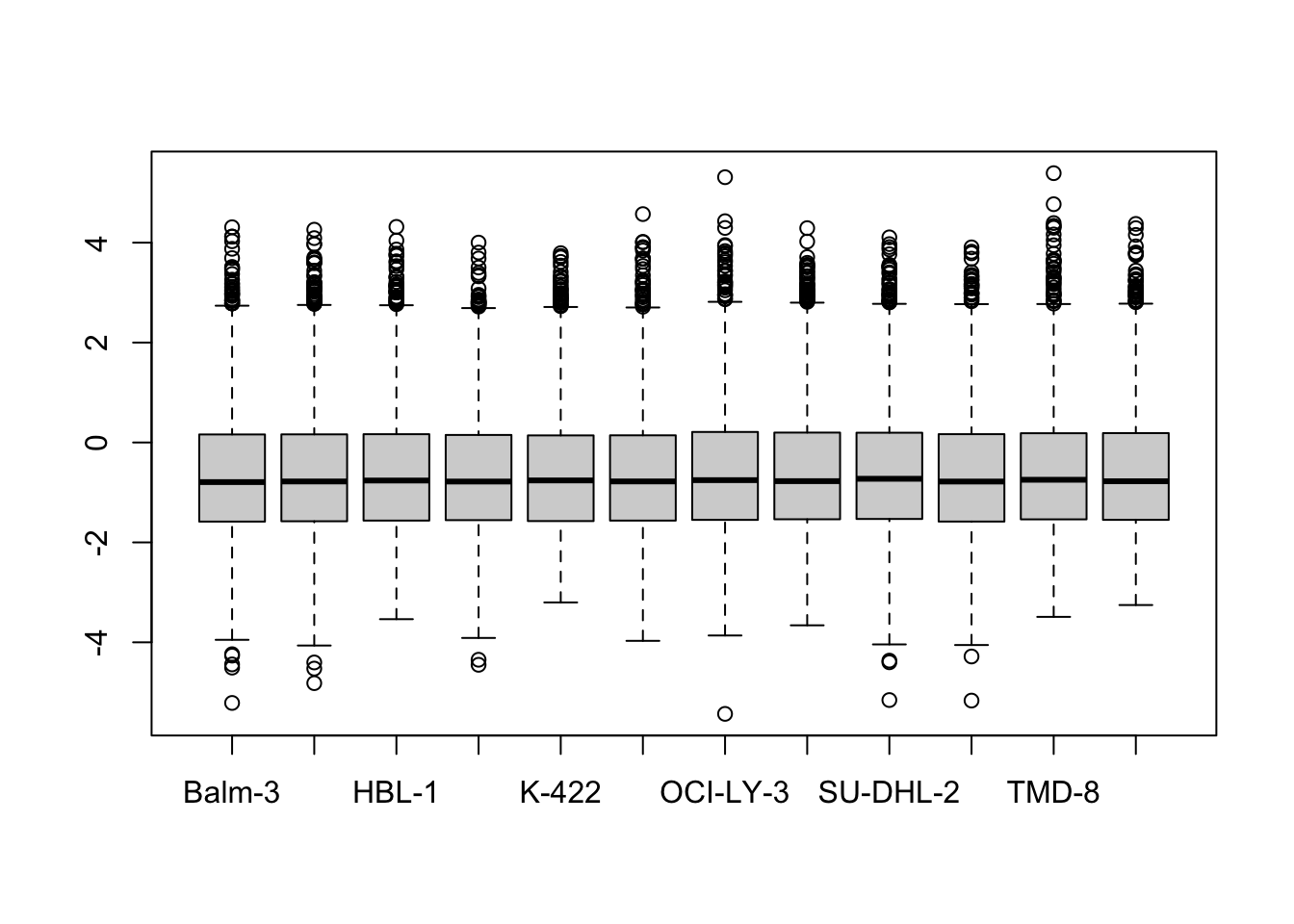

#protNorm <- protData
#assay(protNorm) <- protMatNorm

Create assay experiment object

protTab <- protMatNorm %>% as_tibble(rownames = "uniprotID") %>%
  pivot_longer(-uniprotID, names_to = "cellLine", values_to = "count") %>%
  mutate(cluster = clusterTab[match(cellLine, clusterTab$Name),]$Cluster,
         symbol = uniprotID) %>%
  filter(cellLine %in% clusterTab$Name, 
         !symbol %in% c("",NA), !is.na(cluster))

protSub <- jyluMisc::tidyToSum(protTab, rowID = "uniprotID",colID = "cellLine", 
                     values = "count", annoRow = "symbol", annoCol = "cluster")
#protSub$TP53 <- factor(colAnno[colnames(protSub),]$TP53)

Identify proteins differentially expressed

Differential protein expression using proDA

protMat <- assay(protSub)
fit <- proDA(protMat, design = ~ cluster,
             col_data = colData(protSub))

resTab <- test_diff(fit, contrast = "clusterresistant") %>%
  arrange(pval) %>%
  mutate(symbol = rowData(protSub[name,])$symbol)

resTab.base.embl <- resTab

hist(resTab$pval)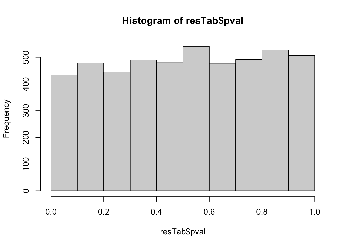

Stronger associations can be observed

Proteins with p-value < 0.05

resTab.sig <- filter(resTab, pval < 0.05)
resTab.sig %>% select(symbol, pval, adj_pval, diff) %>%
  mutate_if(is.numeric, formatC, digits=1) %>%
  DT::datatable()

Plot top 9 examples

pList <- lapply(seq(9), function(i) {
  rec <- resTab.sig[i,]
  plotTab <- tibble(expr = protMat[rec$name,],
                    cluster = protSub$cluster,
                    Name = colnames(protSub)) 
  ggplot(plotTab, aes(x=cluster, y=expr)) +
    geom_boxplot(outlier.shape = NA) +
    ggbeeswarm::geom_quasirandom(aes(color = cluster), size=3) +
    ggrepel::geom_text_repel(aes(label = Name)) +
    ggtitle(rec$symbol) +
    theme_bw() +
    theme(legend.position = "none")
})

cowplot::plot_grid(plotlist = pList,ncol=3)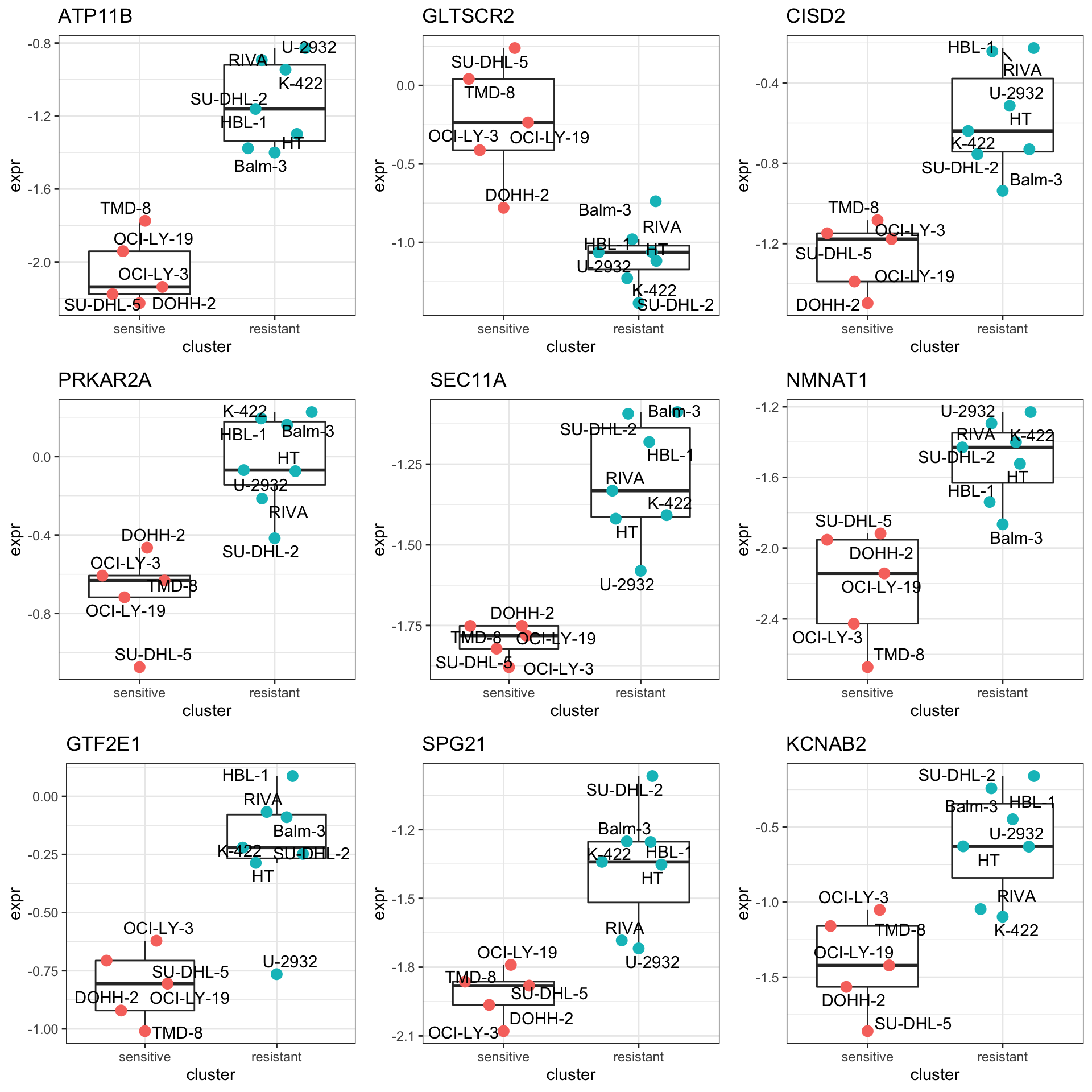

Enrichment analysis

gmts = list(H= "../data/gmts/h.all.v6.2.symbols.gmt",
            KEGG = "../data/gmts/c2.cp.kegg.v6.2.symbols.gmt",
            C6 = "../data/gmts/c6.all.v6.2.symbols.gmt")
inputTab <- resTab %>% filter(pval < 0.1) %>%
  distinct(symbol, .keep_all = TRUE) %>%
  select(symbol, t_statistic) %>% data.frame() %>% column_to_rownames("symbol")
enRes <- list()
enRes[["Hallmark"]] <- runGSEA(inputTab, gmts$H, "page")
enRes[["KEGG"]] <- runGSEA(inputTab, gmts$KEGG,"page")
enRes[["Perturbation"]] <- runGSEA(inputTab, gmts$C6,"page")
p <- plotEnrichmentBar(enRes, pCut =0.05, ifFDR= FALSE)
cowplot::plot_grid(p)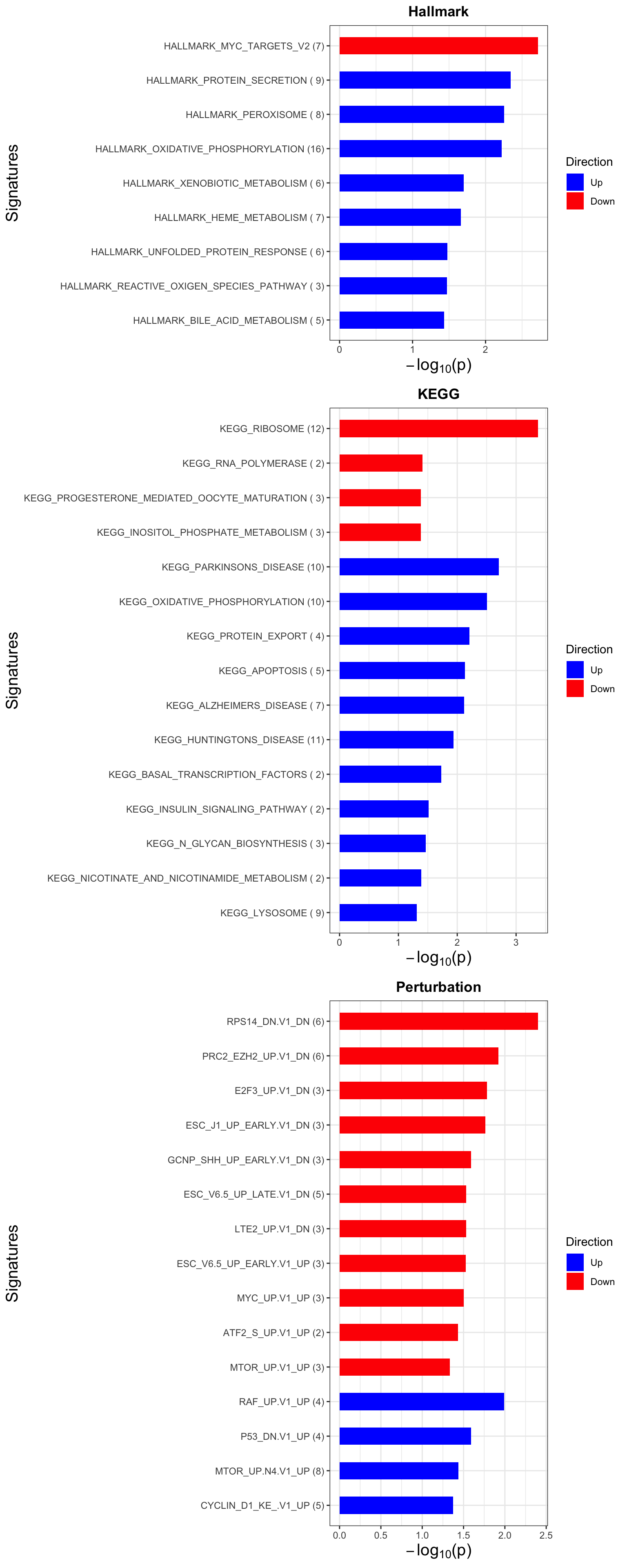

Focus on proteins from Fatty acid metabolism pathway

geneList <- piano::loadGSC(gmts$H)$gsc$HALLMARK_FATTY_ACID_METABOLISM
plotGene <- filter(filter(resTab, pval <= 0.05), symbol%in% geneList )
pList <- lapply(seq(nrow(plotGene)), function(i) {
  rec <- plotGene[i,]
  plotTab <- tibble(expr = protMat[rec$name,],
                    cluster = protSub$cluster) 
  ggplot(plotTab, aes(x=cluster, y=expr)) +
    geom_boxplot(outlier.shape = NA) +
    ggbeeswarm::geom_quasirandom(aes(color = cluster), size=3) +
    ggtitle(rec$symbol) +
    theme_bw()
})

cowplot::plot_grid(plotlist = pList,ncol=3)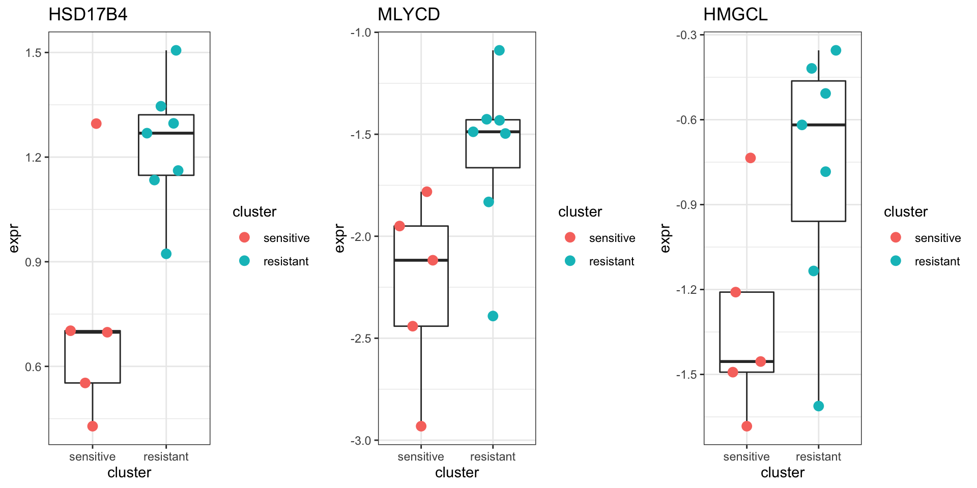

Compare the baseline results from the two datasets

resTab.com <- bind_rows(
  mutate(resTab.base.smart, set ="SMART"),
  mutate(resTab.base.embl, set = "EMBL")
) %>%
  mutate(direction = ifelse(t_statistic >0, "Up_in_resistant", "Down_in_resistant")) %>%
  select(symbol, set, direction, pval)

Plot p-values

plotTab <- resTab.com %>%
  group_by(symbol, set, direction) %>%
  summarise(pval = min(pval)) %>%
  pivot_wider(names_from = set, values_from = pval) %>%
  filter(!is.na(SMART),!is.na(EMBL)) %>%
  mutate(sig = case_when(
    EMBL <= 0.05 & SMART <= 0.05 ~ "both",
    EMBL <= 0.05 & SMART >= 0.05 ~ "only EMBL",
    EMBL >= 0.05 & SMART <= 0.05 ~ "only SMART"
  ))

#how many commonly detected proteins?
nrow(plotTab)

[1] 1906

ggplot(plotTab, aes(x=-log10(SMART),y=-log10(EMBL))) +
  geom_point(aes(col = sig)) +
  geom_smooth(method = "lm") +
  facet_wrap(~direction) +
  ggrepel::geom_text_repel(data = filter(plotTab, sig == "both"), aes(label = symbol)) +
  theme_bw()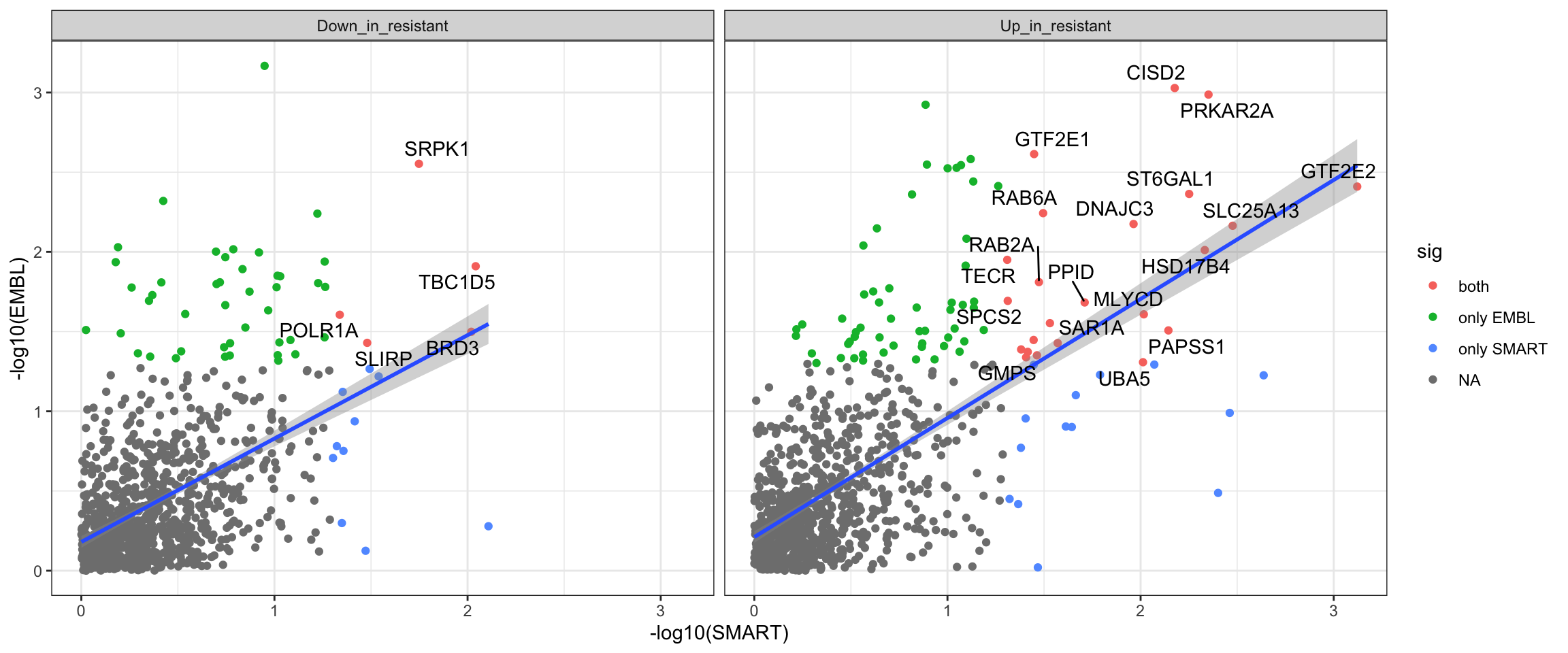

Metabolimics

Process metabolomic data

Normalization (not performed)

metaData <- readRDS("../data/SC005_SummarizedExperiment_metabolomics.RDS")
metaData <- metaData[,metaData$cell.line %in% clusterTab$Name]
metaMat <- assay(metaData)
boxplot(metaMat)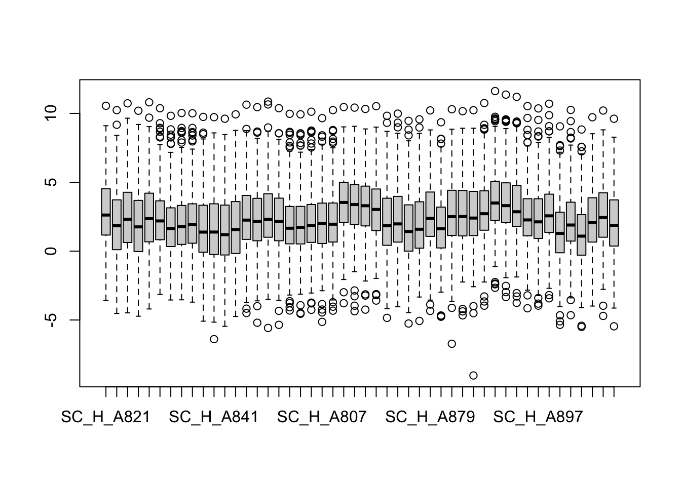

#metaMatNorm <- PhosR::medianScaling(metaMat, scale = FALSE)
metaMatNorm <- metaMat
#boxplot(metaMatNorm)
metaNorm <- metaData
assay(metaNorm) <- metaMatNorm
assayNames(metaNorm) <- "norm"

Average technical replicates for each cell line

metaTab <- jyluMisc::sumToTidy(metaNorm) %>%
  group_by(cell.line, rowID, metabolite, class, condition) %>%
  summarise(count = mean(norm, na.rm=TRUE)) %>%
  dplyr::rename(symbol = metabolite, cellLine = cell.line) %>%
  mutate(colID = paste0(cellLine,"_", condition)) %>%
  ungroup()

metaAll <- jyluMisc::tidyToSum(metaTab, rowID = "rowID", colID = "colID", 
                     values = "count", annoRow = "symbol", 
                     annoCol = c("condition", "cellLine"))

#add additional annotations
metaAll$cluster <- clusterTab[match(metaAll$cellLine, clusterTab$Name),]$Cluster
metaAll$TP53 <- clusterTab[match(metaAll$cellLine, clusterTab$Name),]$TP53

#remove uncessary samples and records
metaAll <- metaAll[!rowData(metaAll)$symbol %in% c("",NA), !is.na(metaAll$cluster)]
dim(metaAll)

[1] 286  24

colData(metaAll) %>% data.frame() %>% DT::datatable()

Differential expression in Baseline (Untreated) condition

metaSub <- metaAll[,metaAll$condition == "U"]

Differential metabolites abundance

metaMat <- assay(metaSub)
designMat <- model.matrix(~metaSub$cluster)
fit <- lmFit(metaMat, designMat)
fit2 <- eBayes(fit)

resTab <- topTable(fit2, number= Inf) %>%
  dplyr::rename(pval = P.Value, adj_pval = adj.P.Val) %>%
  arrange(pval) %>%
  as_tibble(rownames = "name") %>%
  mutate(symbol = rowData(metaSub[name,])$symbol)

hist(resTab$pval)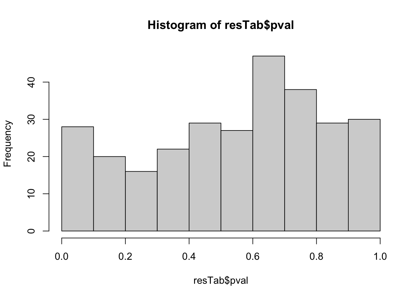

Not strong difference

Show all metabolites

resTab.sig <- filter(resTab)
resTab.sig %>% select(symbol, pval, adj_pval, logFC, t) %>%
  mutate_if(is.numeric, formatC, digits=1) %>%
  DT::datatable()

Plot top 9 examples

pList <- lapply(seq(9), function(i) {
  rec <- resTab.sig[i,]
  plotTab <- tibble(expr = metaMat[rec$name,],
                    cluster = metaSub$cluster,
                    TP53 = metaSub$TP53,
                    Name = colnames(metaSub)) 
  ggplot(plotTab, aes(x=cluster, y=expr)) +
    geom_boxplot(outlier.shape = NA) +
    geom_point(aes(color = cluster, shape = TP53), size=3) +
    ggrepel::geom_text_repel(aes(label = Name)) +
    ggtitle(rec$symbol) +
    theme_bw() +
    theme(legend.position = "none")
})

cowplot::plot_grid(plotlist = pList,ncol=3)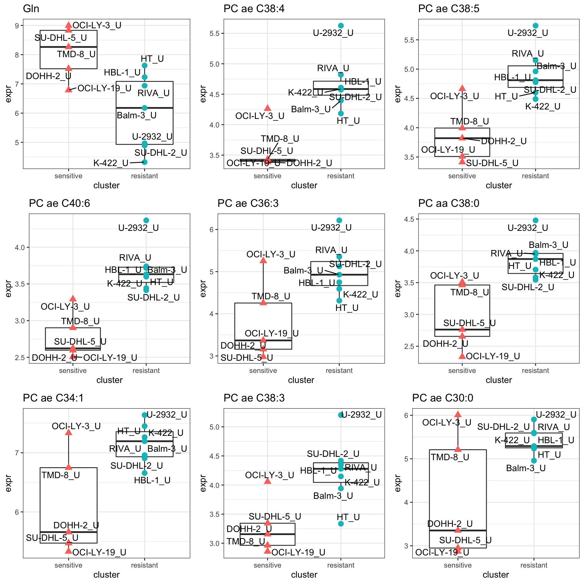

Differential expression in treated (T) condition

metaSub <- metaAll[,metaAll$condition == "T"]

Differential metabolites abundance

metaMat <- assay(metaSub)
designMat <- model.matrix(~metaSub$cluster)
fit <- lmFit(metaMat, designMat)
fit2 <- eBayes(fit)

resTab <- topTable(fit2, number= Inf) %>%
  dplyr::rename(pval = P.Value, adj_pval = adj.P.Val) %>%
  arrange(pval) %>%
  as_tibble(rownames = "name") %>%
  mutate(symbol = rowData(metaSub[name,])$symbol)

hist(resTab$pval)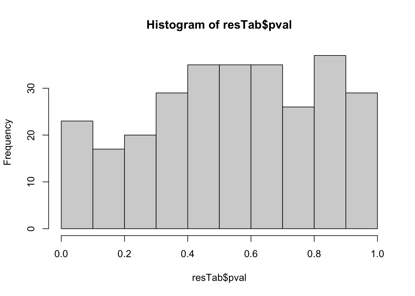

Not strong difference

Metabolites with p-value < 0.05

resTab.sig <- filter(resTab, pval < 0.05)
resTab.sig %>% select(symbol, pval, adj_pval, logFC, t) %>%
  mutate_if(is.numeric, formatC, digits=1) %>%
  DT::datatable()

Plot top 9 examples

pList <- lapply(seq(9), function(i) {
  rec <- resTab.sig[i,]
  plotTab <- tibble(expr = metaMat[rec$name,],
                    cluster = metaSub$cluster,
                    TP53 = metaSub$TP53,
                    Name = colnames(metaSub)) 
  ggplot(plotTab, aes(x=cluster, y=expr)) +
    geom_boxplot(outlier.shape = NA) +
    geom_point(aes(color = cluster, shape = TP53), size=3) +
    ggrepel::geom_text_repel(aes(label = Name)) +
    ggtitle(rec$symbol) +
    theme_bw() +
    theme(legend.position = "none")
})

cowplot::plot_grid(plotlist = pList,ncol=3)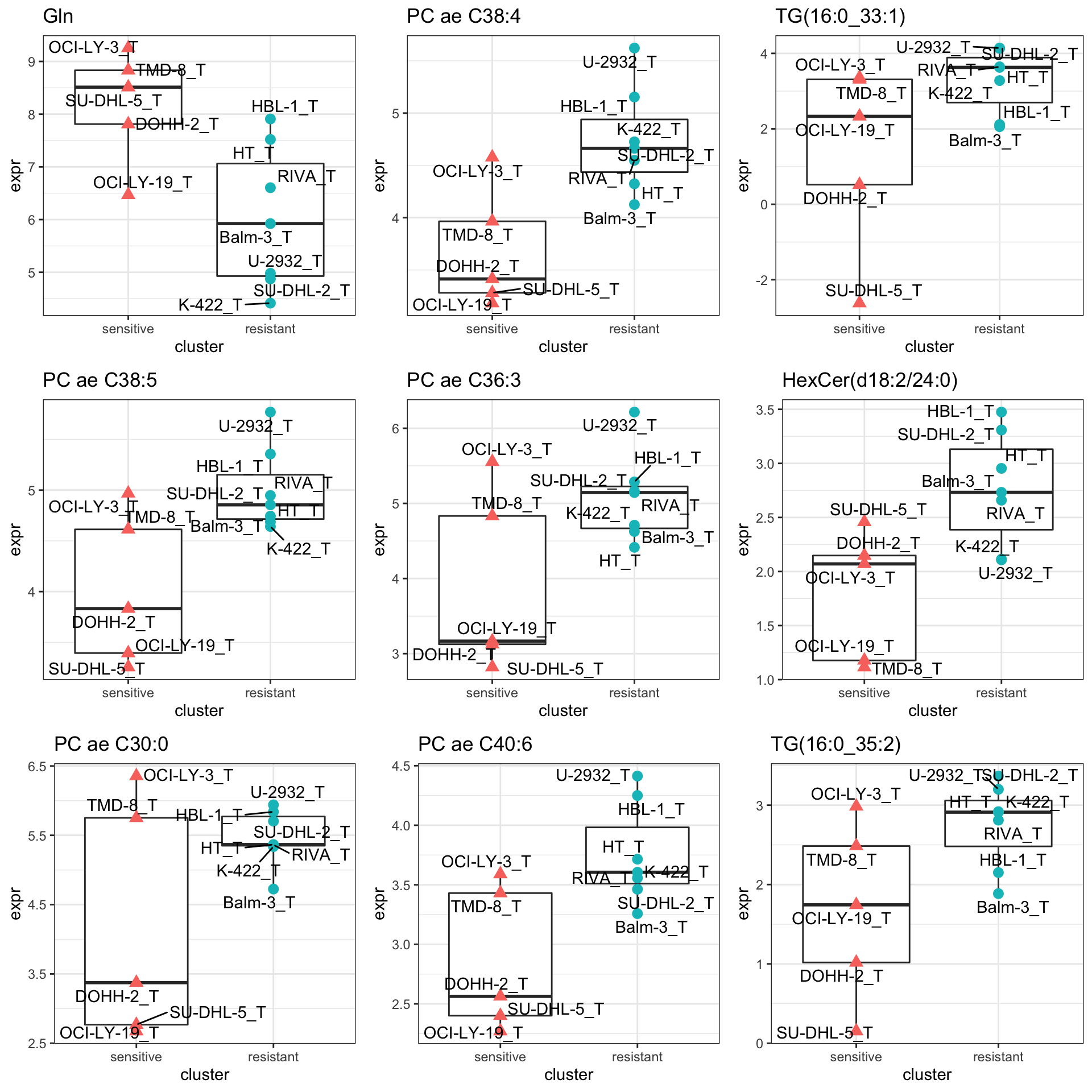

Differential expression before and after treatment

metaSub <- metaAll

Differential metabolites abundance

metaMat <- assay(metaSub)
designMat <- model.matrix(~cellLine + condition, colData(metaSub))
fit <- lmFit(metaMat, designMat)
fit2 <- eBayes(fit)

resTab <- topTable(fit2, number= Inf, coef = "conditionT") %>%
  dplyr::rename(pval = P.Value, adj_pval = adj.P.Val) %>%
  arrange(pval) %>%
  as_tibble(rownames = "name") %>%
  mutate(symbol = rowData(metaSub[name,])$symbol)

hist(resTab$pval)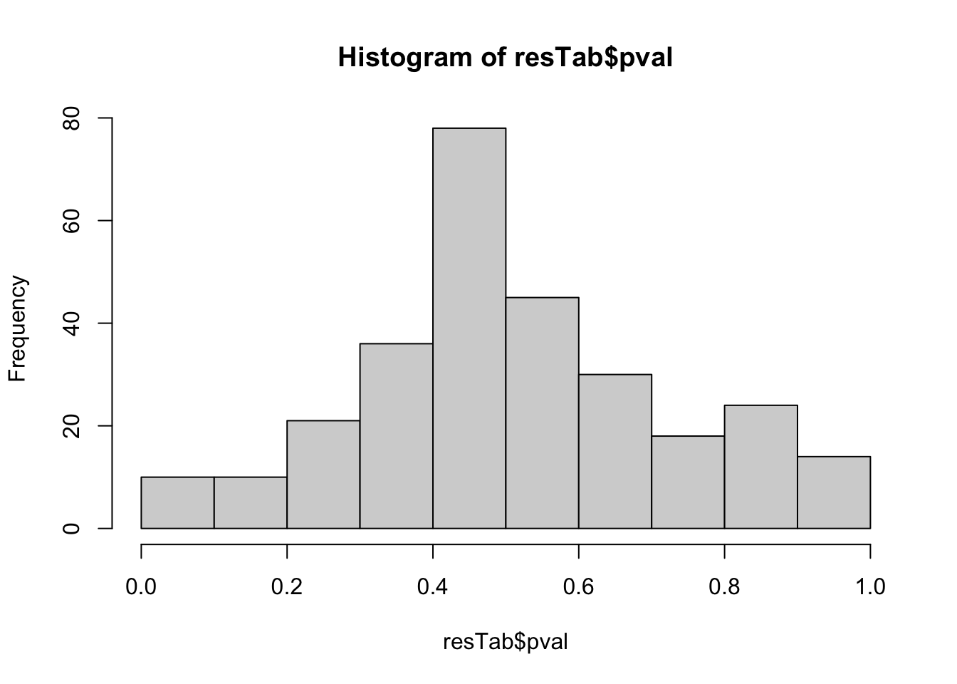

Some difference can be detected

Proteins with p-value < 0.05

resTab.sig <- filter(resTab, pval < 0.05)
resTab.sig %>% select(symbol, pval, adj_pval, logFC, t) %>%
  mutate_if(is.numeric, formatC, digits=1) %>%
  DT::datatable()

Plot top 9 examples

pList <- lapply(seq(5), function(i) {
  rec <- resTab.sig[i,]
  plotTab <- tibble(expr = metaMat[rec$name,],
                    cluster = metaSub$cluster,
                    Name = metaSub$cellLine,
                    condition = metaSub$condition) 
  ggplot(plotTab, aes(x=condition, y=expr)) +
    geom_boxplot(outlier.shape = NA) +
    geom_point(aes(color = cluster), size=3) +
    geom_line(aes(group = Name), linetype = "dotted") +
    ggrepel::geom_text_repel(aes(label = Name)) +
    ggtitle(rec$symbol) +
    theme_bw()
})

cowplot::plot_grid(plotlist = pList,ncol=3)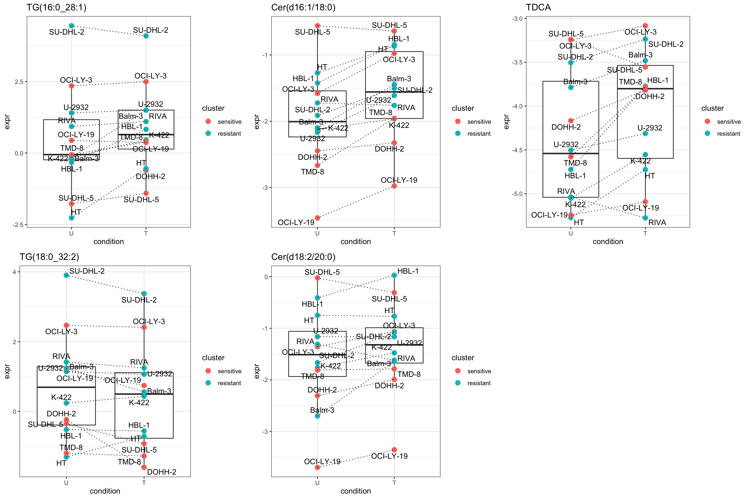

Interaction between treatment and sensitivity cluster

metaSub <- metaAll

Differential protein expression using proDA

metaMat <- assay(metaSub)
design <- model.matrix(~ 0 + condition*cluster, data = colData(metaSub)) 
colnames(design) <- make.names(colnames(design))

cor <- duplicateCorrelation(metaMat, design, block=metaSub$cellLine)
#cor$consensus.correlation

fit <- lmFit(object=metaMat, design=design, block=metaSub$cellLine,
    correlation = cor$consensus.correlation, method = "ls")
fit2 <- eBayes(fit)
resTab  <- topTable(fit2, number = Inf, coef="conditionT.clusterresistant") %>%
  as_tibble(rownames = "name") %>%
  mutate(symbol = rowData(metaSub[name,])$symbol) %>%
  dplyr::rename(pval = P.Value, adj_pval = adj.P.Val, diff = logFC, t_statistics = t)

hist(resTab$pval)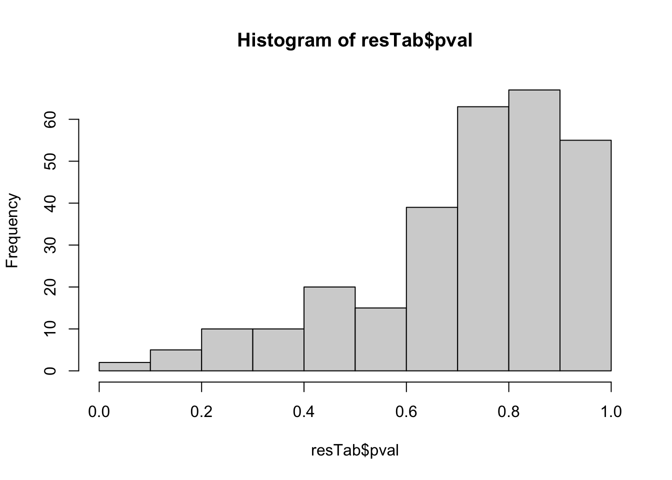

Not strong difference

Proteins with p-value < 0.05

resTab.sig <- filter(resTab, pval < 0.05)
resTab.sig %>% select(symbol, pval, adj_pval, diff) %>%
  mutate_if(is.numeric, formatC, digits=1) %>%
  DT::datatable()

Plot top 9 examples

pList <- lapply(seq(9), function(i) {
  rec <- resTab.sig[i,]
  plotTab <- tibble(expr = metaMat[rec$name,],
                    cluster = metaSub$cluster,
                    Name = metaSub$cellLine,
                    condition = metaSub$condition) 
  ggplot(plotTab, aes(x=condition, y=expr)) +
    geom_boxplot(outlier.shape = NA) +
    geom_point(aes(color = cluster), size=3) +
    geom_line(aes(group = Name), linetype = "dotted") +
    ggrepel::geom_text_repel(aes(label = Name)) +
    ggtitle(rec$symbol) +
    theme_bw() +
    facet_wrap(~cluster)
})

cowplot::plot_grid(plotlist = pList,ncol=3)

Differential gene expression analysis based on public data

Proprocessing

load("../data/DepMap_GEXwide.RData")
exprMat <- t(DepMap_GEXwide)
exprMat <- exprMat[,colnames(exprMat) %in% clusterTab$Name]

# Remove low count genes
exprMat <- exprMat[rowMedians(exprMat) >0,]

dim(exprMat)

[1] 15551     7

boxplot(exprMat)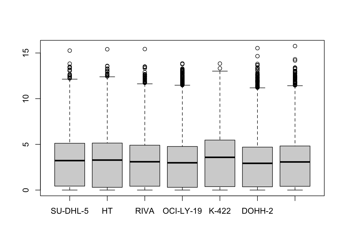

vstObj <- vsn::vsnMatrix(exprMat)
exprMat <- vsn::predict(vstObj, exprMat)

boxplot(exprMat)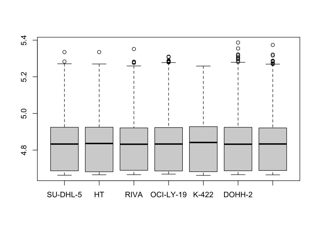

#save process data
#save(exprMat, file = "gene_exprMat.RData")

Differential expression using limma

colTab <- clusterTab[match(colnames(exprMat), clusterTab$Name),] %>%
  column_to_rownames("Name") %>% data.frame()
designMat <- model.matrix(~Cluster, colTab)

fit <- lmFit(exprMat, designMat)
fit2 <- eBayes(fit)
resTab <- topTable(fit2, number = Inf) %>%
  as_tibble(rownames = "symbol")

Associations with p <= 0.05

resTab.sig <- filter(resTab, P.Value <= 0.05)
resTab.sig %>% mutate_if(is.numeric, formatC, digits=2) %>% DT::datatable()

Plot top 9 examples

pList <- lapply(seq(9), function(i) {
  rec <- resTab.sig[i,]
  plotTab <- tibble(expr = exprMat[rec$symbol,],
                    cluster = colTab$Cluster,
                    TP53 = colTab$TP53,
                    Name = colnames(exprMat)) 
  ggplot(plotTab, aes(x=cluster, y=expr)) +
    geom_boxplot(outlier.shape = NA) +
    geom_point(aes(color = cluster), size=3) +
    ggrepel::geom_text_repel(aes(label = Name)) +
    ggtitle(rec$symbol) +
    theme_bw() +
    theme(legend.position = "none")
})

cowplot::plot_grid(plotlist = pList,ncol=3)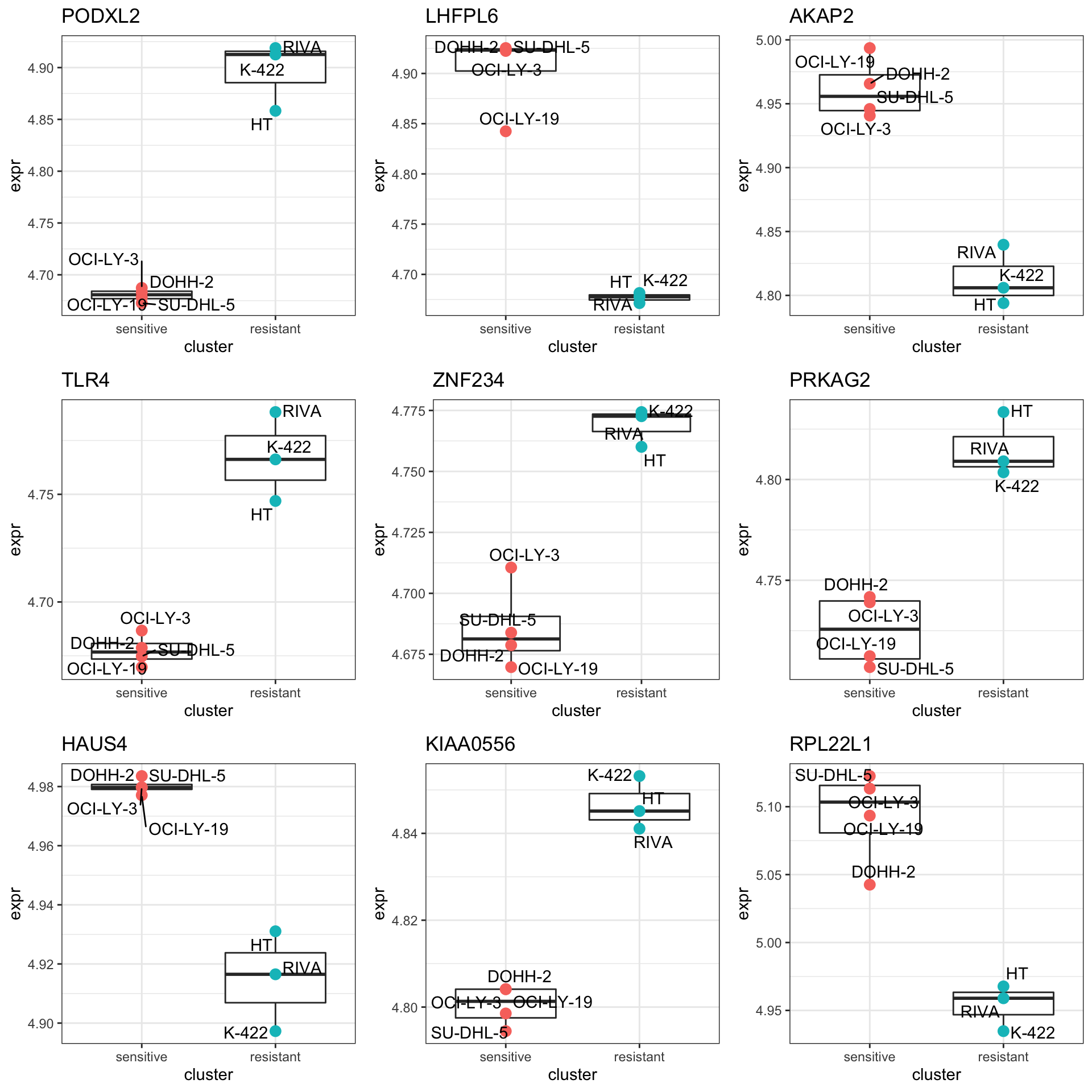

Enrichment analysis

gmts = list(H= "../data/gmts/h.all.v6.2.symbols.gmt",
            KEGG = "../data/gmts/c2.cp.kegg.v6.2.symbols.gmt",
            C6 = "../data/gmts/c6.all.v6.2.symbols.gmt")
inputTab <- resTab %>% filter(P.Value < 0.1) %>%
  distinct(symbol, .keep_all = TRUE) %>%
  select(symbol, t) %>% data.frame() %>% column_to_rownames("symbol")
enRes <- list()
enRes[["Hallmark"]] <- runGSEA(inputTab, gmts$H, "page")
enRes[["KEGG"]] <- runGSEA(inputTab, gmts$KEGG,"page")
enRes[["Perturbation"]] <- runGSEA(inputTab, gmts$C6,"page")
p <- plotEnrichmentBar(enRes, pCut =0.01, ifFDR= FALSE)
cowplot::plot_grid(p)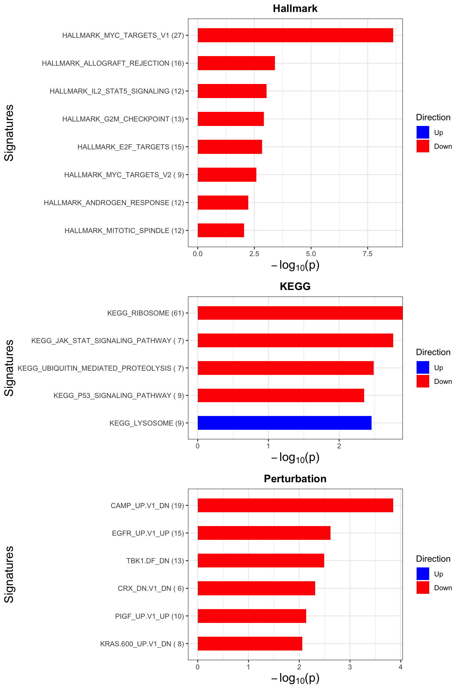

Focus on proteins from Fatty acid metabolism pathway

geneList <- piano::loadGSC(gmts$H)$gsc$HALLMARK_FATTY_ACID_METABOLISM
plotGene <- filter(filter(resTab, P.Value <= 0.05), symbol%in% geneList )
pList <- lapply(seq(nrow(plotGene)), function(i) {
  rec <- plotGene[i,]
  plotTab <- tibble(expr = exprMat[rec$symbol,],
                    cluster = colTab$Cluster,
                    TP53 = colTab$TP53) 
  ggplot(plotTab, aes(x=cluster, y=expr)) +
    geom_boxplot(outlier.shape = NA) +
    ggbeeswarm::geom_quasirandom(aes(color = cluster, shape = TP53), size=3) +
    ggtitle(rec$symbol) +
    theme_bw()
})

cowplot::plot_grid(plotlist = pList,ncol=3)

Session information

sessionInfo()

R version 4.2.0 (2022-04-22)
Platform: x86_64-apple-darwin17.0 (64-bit)
Running under: macOS Big Sur/Monterey 10.16

Matrix products: default
BLAS:   /Library/Frameworks/R.framework/Versions/4.2/Resources/lib/libRblas.0.dylib
LAPACK: /Library/Frameworks/R.framework/Versions/4.2/Resources/lib/libRlapack.dylib

locale:
[1] en_US.UTF-8/en_US.UTF-8/en_US.UTF-8/C/en_US.UTF-8/en_US.UTF-8

attached base packages:
[1] stats4    stats     graphics  grDevices utils     datasets  methods  
[8] base     

other attached packages:
 [1] piano_2.12.0                forcats_0.5.1              
 [3] stringr_1.4.0               dplyr_1.0.9                
 [5] purrr_0.3.4                 readr_2.1.2                
 [7] tidyr_1.2.0                 tibble_3.1.8               
 [9] ggplot2_3.3.6               tidyverse_1.3.2            
[11] proDA_1.10.0                DESeq2_1.36.0              
[13] SummarizedExperiment_1.26.1 Biobase_2.56.0             
[15] GenomicRanges_1.48.0        GenomeInfoDb_1.32.2        
[17] IRanges_2.30.0              S4Vectors_0.34.0           
[19] BiocGenerics_0.42.0         MatrixGenerics_1.8.1       
[21] matrixStats_0.62.0          limma_3.52.2               
[23] jyluMisc_0.1.5             

loaded via a namespace (and not attached):
  [1] utf8_1.2.2             shinydashboard_0.7.2   tidyselect_1.1.2      
  [4] RSQLite_2.2.15         AnnotationDbi_1.58.0   htmlwidgets_1.5.4     
  [7] grid_4.2.0             BiocParallel_1.30.3    maxstat_0.7-25        
 [10] munsell_0.5.0          preprocessCore_1.58.0  codetools_0.2-18      
 [13] statmod_1.4.36         DT_0.23                withr_2.5.0           
 [16] colorspace_2.0-3       highr_0.9              knitr_1.39            
 [19] rstudioapi_0.13        ggsignif_0.6.3         labeling_0.4.2        
 [22] git2r_0.30.1           slam_0.1-50            GenomeInfoDbData_1.2.8
 [25] KMsurv_0.1-5           bit64_4.0.5            farver_2.1.1          
 [28] rprojroot_2.0.3        vctrs_0.4.1            generics_0.1.3        
 [31] TH.data_1.1-1          xfun_0.31              sets_1.0-21           
 [34] R6_2.5.1               ggbeeswarm_0.6.0       locfit_1.5-9.6        
 [37] bitops_1.0-7           cachem_1.0.6           fgsea_1.22.0          
 [40] DelayedArray_0.22.0    assertthat_0.2.1       promises_1.2.0.1      
 [43] scales_1.2.0           multcomp_1.4-19        googlesheets4_1.0.0   
 [46] beeswarm_0.4.0         gtable_0.3.0           extraDistr_1.9.1      
 [49] affy_1.74.0            sandwich_3.0-2         workflowr_1.7.0       
 [52] rlang_1.0.4            genefilter_1.78.0      splines_4.2.0         
 [55] rstatix_0.7.0          gargle_1.2.0           broom_1.0.0           
 [58] BiocManager_1.30.18    yaml_2.3.5             abind_1.4-5           
 [61] modelr_0.1.8           crosstalk_1.2.0        backports_1.4.1       
 [64] httpuv_1.6.5           tools_4.2.0            relations_0.6-12      
 [67] affyio_1.66.0          ellipsis_0.3.2         gplots_3.1.3          
 [70] jquerylib_0.1.4        RColorBrewer_1.1-3     Rcpp_1.0.9            
 [73] visNetwork_2.1.0       zlibbioc_1.42.0        RCurl_1.98-1.7        
 [76] ggpubr_0.4.0           cowplot_1.1.1          zoo_1.8-10            
 [79] haven_2.5.0            ggrepel_0.9.1          cluster_2.1.3         
 [82] exactRankTests_0.8-35  fs_1.5.2               magrittr_2.0.3        
 [85] data.table_1.14.2      reprex_2.0.1           survminer_0.4.9       
 [88] googledrive_2.0.0      mvtnorm_1.1-3          hms_1.1.1             
 [91] shinyjs_2.1.0          mime_0.12              evaluate_0.15         
 [94] xtable_1.8-4           XML_3.99-0.10          readxl_1.4.0          
 [97] gridExtra_2.3          compiler_4.2.0         KernSmooth_2.23-20    
[100] crayon_1.5.1           htmltools_0.5.3        mgcv_1.8-40           
[103] later_1.3.0            tzdb_0.3.0             geneplotter_1.74.0    
[106] lubridate_1.8.0        DBI_1.1.3              dbplyr_2.2.1          
[109] MASS_7.3-58            Matrix_1.4-1           car_3.1-0             
[112] cli_3.3.0              vsn_3.64.0             marray_1.74.0         
[115] parallel_4.2.0         igraph_1.3.4           pkgconfig_2.0.3       
[118] km.ci_0.5-6            xml2_1.3.3             annotate_1.74.0       
[121] vipor_0.4.5            bslib_0.4.0            XVector_0.36.0        
[124] drc_3.0-1              rvest_1.0.2            digest_0.6.29         
[127] Biostrings_2.64.0      rmarkdown_2.14         cellranger_1.1.0      
[130] fastmatch_1.1-3        survMisc_0.5.6         shiny_1.7.2           
[133] gtools_3.9.3           nlme_3.1-158           lifecycle_1.0.1       
[136] jsonlite_1.8.0         carData_3.0-5          fansi_1.0.3           
[139] pillar_1.8.0           lattice_0.20-45        KEGGREST_1.36.3       
[142] fastmap_1.1.0          httr_1.4.3             plotrix_3.8-2         
[145] survival_3.3-1         glue_1.6.2             png_0.1-7             
[148] bit_4.0.4              stringi_1.7.8          sass_0.4.2            
[151] blob_1.2.3             caTools_1.18.2         memoise_2.0.1