Last updated: 2022-07-08

Checks: 4 2

Knit directory: combiDLBCL/analysis/

This reproducible R Markdown analysis was created with workflowr (version 1.7.0). The Checks tab describes the reproducibility checks that were applied when the results were created. The Past versions tab lists the development history.

Environment: empty

Great job! The global environment was empty. Objects defined in the global environment can affect the analysis in your R Markdown file in unknown ways. For reproduciblity it’s best to always run the code in an empty environment.

Seed: set.seed(20220425)

The command set.seed(20220425) was run prior to running the code in the R Markdown file. Setting a seed ensures that any results that rely on randomness, e.g. subsampling or permutations, are reproducible.

Session information: recorded

Great job! Recording the operating system, R version, and package versions is critical for reproducibility.

Cache: detected

The following chunks had caches available:

unnamed-chunk-80
unnamed-chunk-84
unnamed-chunk-88
unnamed-chunk-92
unnamed-chunk-96

To ensure reproducibility of the results, delete the cache directory Doxo_resistant_cache and re-run the analysis. To have workflowr automatically delete the cache directory prior to building the file, set delete_cache = TRUE when running wflow_build() or wflow_publish().

File paths: relative

Great job! Using relative paths to the files within your workflowr project makes it easier to run your code on other machines.

Repository version: no version control

Tracking code development and connecting the code version to the results is critical for reproducibility. To start using Git, open the Terminal and type git init in your project directory.

This project is not being versioned with Git. To obtain the full reproducibility benefits of using workflowr, please see ?wflow_start.

Load libraries and datasets

Data preprocessing

Drug screen data (the cell line screen data from Tobias)

Read data

load("../data/Screen.CL19.RData")

screenData <- filter(Screen.CL19, str_detect(Entity, "DLBCL"), Drug == "Doxorubicine", TimePoint == "48 h") %>%
  mutate(Subtype = str_remove(Entity,"DLBCL ")) %>%
  select(Name, Drug.Conc, Duplicate, Normalized, Subtype)

Using 48h Doxorubicin treatment response as the continous response variable

Some cell lines have duplicates, check the reproducibility

dupCell <- unique(filter(screenData, Duplicate == "2")$Name)
compareTab <- filter(screenData, Name %in% dupCell) %>%
  mutate(Duplicate = paste0("R",Duplicate)) %>%
  pivot_wider(names_from = Duplicate, values_from = Normalized)

ggplot(compareTab, aes(x=R1, y=R2, col = factor(Drug.Conc))) +
  geom_point() +
  geom_abline(intercept = 0, slope = 1, col = "red") +
  facet_grid(~Name)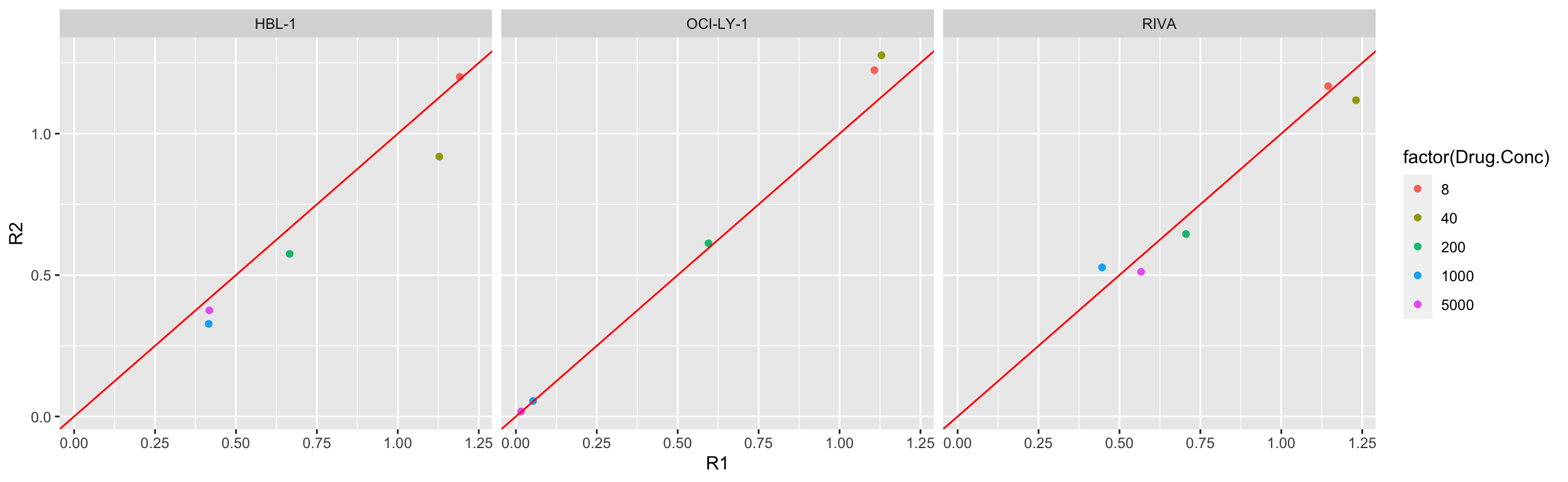

Look fine, the duplicates can be averaged.

screenData <- group_by(screenData, Name, Drug.Conc, Subtype) %>%
  summarise(normVal = mean(Normalized)) %>%
  ungroup()

Dose response of Doxorubicin in DLBCL cell lines

plotTab <- screenData 
p <- ggplot(plotTab, aes(x=Drug.Conc, y=normVal, group = Name, col = Name)) +
    geom_line() + geom_point() +
    scale_x_log10() + theme_bw() +
    coord_cartesian(ylim = c(0,1.5)) +
    #ggtitle(paste0(rec$Drug_B)) +
    theme(legend.position = "right") 
p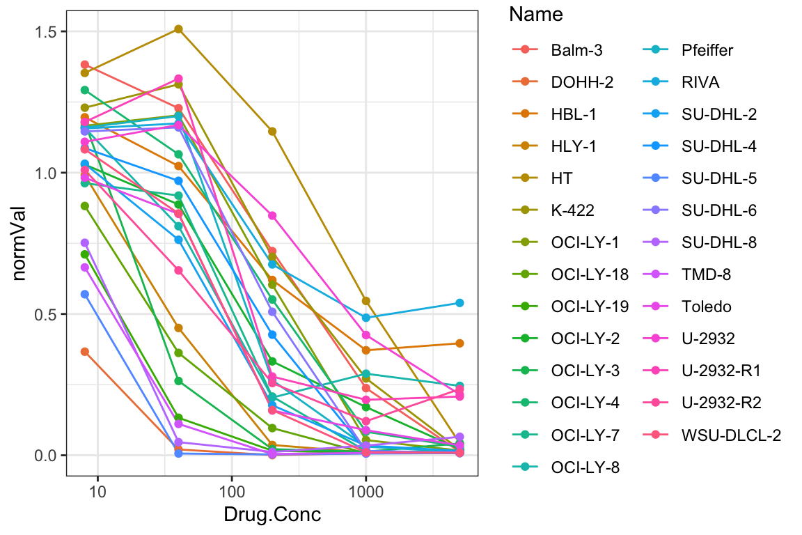

It’s difficult to define resistant and sensitive groups. Better to use continues response based on AUC

aucTab <- screenData %>% group_by(Name,Subtype) %>%
  summarise(auc = calcAUC(normVal, Drug.Conc)) %>%
  ungroup() %>%
  arrange(auc) %>% 
  mutate(Name = factor(Name, levels = Name)) 

ggplot(aucTab, aes(x=Name, y=auc, col = Subtype)) +
  geom_point() +
  theme(axis.text.x = element_text(angle = 90, hjust = 1, vjust = 0.5))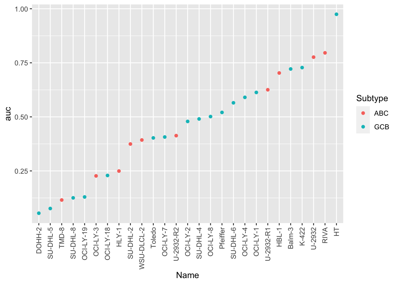

Whether Doxorubicine response is associated with ABC/GCB subtype?

ggplot(aucTab, aes(x=Subtype, y = auc)) +
  geom_boxplot() + geom_point()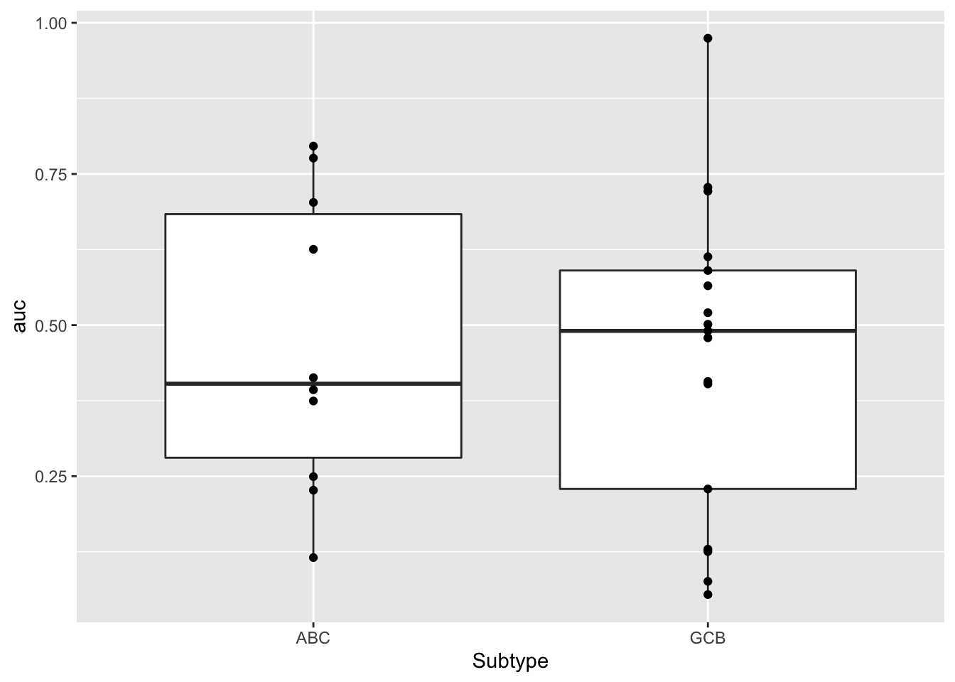

t.test(auc~Subtype, aucTab)


    Welch Two Sample t-test

data:  auc by Subtype
t = 0.20033, df = 19.886, p-value = 0.8433
alternative hypothesis: true difference in means between group ABC and group GCB is not equal to 0
95 percent confidence interval:
 -0.1863762  0.2259621
sample estimates:
mean in group ABC mean in group GCB 
        0.4673122         0.4475192

Genomics

Processing genomics data

Load genomics

load("../data/SVs_filtered.RData")
svTab <- filter(svTab, Name %in% aucTab$Name)

Summarise mutations: count as gene mutation if there is at least one mutation within gene

mutTab <- group_by(svTab, Name, Gene) %>% summarise(n = length(Name)) %>%
  arrange(desc(n))

#Get mutations occured at least in three cell lines
geneCount <- group_by(mutTab, Gene) %>% summarise(n=length(Name)) %>%
  filter(n>=3) %>% arrange(desc(n)) %>%
  mutate(Gene = factor(Gene, levels = Gene))

There are too many mutations. Manual curation maybe needed.

Occurrence of mutations among cell lines, only mutations occurred at least 3 times are considered

ggplot(geneCount, aes(x=Gene, y=n)) +
  geom_bar(stat = "identity") +
  theme_bw() + theme(axis.text.x = element_text(angle = 90, hjust = 1, vjust = 0.5))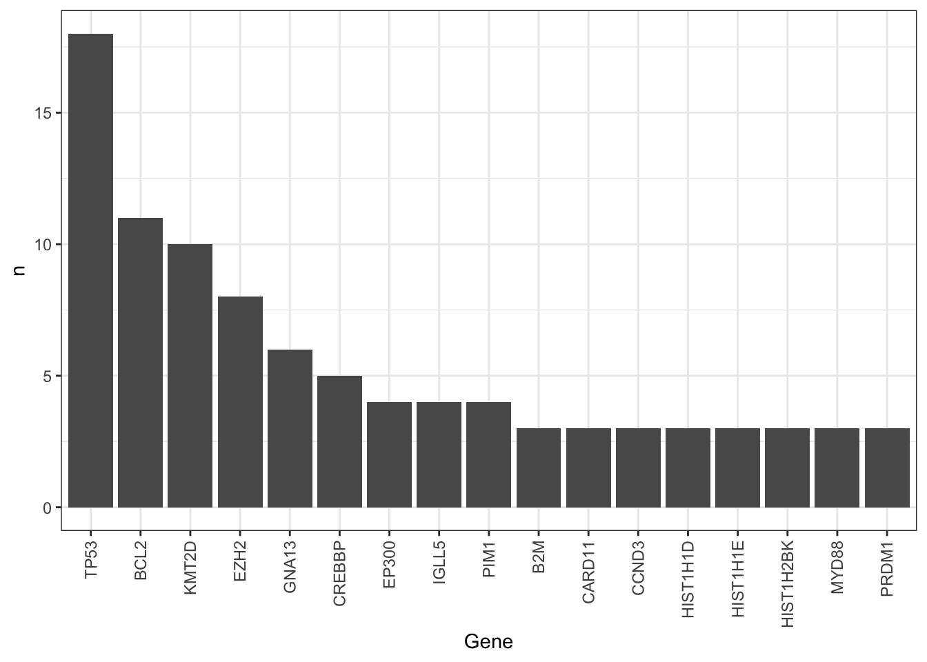

T-test

geneTab <- filter(mutTab, Gene %in% geneCount$Gene) %>%
  mutate(status =1) %>% select(Name, Gene, status) %>%
  pivot_wider(names_from = "Gene", values_from = "status") %>%
  mutate_all(replace_na,0) %>%
  pivot_longer(-Name, names_to = "Gene", values_to = "status") %>%
  ungroup()

testTab <- left_join(geneTab, aucTab, by = "Name")
geneMat <- geneTab %>% pivot_wider(names_from = Name, values_from = status) %>%
  column_to_rownames("Gene") %>% as.matrix()
omicList <- list(gene = geneMat)

resTab <- group_by(testTab, Gene) %>% nest() %>%
  mutate(m = map(data, ~t.test(auc~status,.))) %>%
  mutate(res = map(m, broom::tidy)) %>%
  unnest(res) %>%
  select(Gene, p.value) %>%
  arrange(p.value)
head(resTab)

# A tibble: 6 × 2
# Groups:   Gene [6]
  Gene      p.value
  <chr>       <dbl>
1 TP53     0.000279
2 EZH2     0.0510  
3 PRDM1    0.0529  
4 KMT2D    0.114   
5 PIM1     0.237   
6 HIST1H1E 0.353

TP53 is the most significant one

Dose response of Doxorubicine with TP53 annotated

plotTab <- screenData %>%
  left_join(filter(geneTab, Gene == "TP53"), by = "Name") %>%
  mutate(TP53 = case_when(
    status == 0 ~ "WT",
    status == 1 ~ "Mut"
  ))
p <- ggplot(plotTab, aes(x=Drug.Conc, y=normVal, 
                         group = Name, col = factor(TP53))) +
    geom_line() + geom_point() +
    scale_x_log10() + theme_bw() +
    coord_cartesian(ylim = c(0,1.5)) +
    theme(legend.position = "right")
p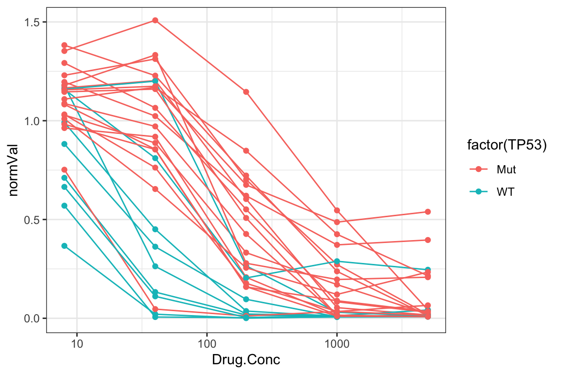

Add TP53 status to the AUC table

aucTab <- aucTab %>% 
  left_join(filter(geneTab, Gene == "TP53"), by = "Name") %>%
  mutate(TP53 = case_when(
    status == 0 ~ "WT",
    status == 1 ~ "Mut"
  )) %>%
  select(-Gene, -status) %>%
  arrange(auc) 

plotTab <- aucTab %>% mutate(Name = factor(Name, levels = Name))
ggplot(plotTab, aes(x=Name,y=auc,col=TP53)) +
  geom_point() +
  theme(axis.text.x = element_text(angle = 90, hjust =1, vjust = 0.5))

The response is mostly accord with TP53 mutation status. Only a few cell lines are outliers:
SU-DHL-8 is TP53 mutated, but also sensitive.
OCI-LY-8 and Pfeffer are WT but rather resistant to Doxorubicine

Association with proteomics

Preprocessing proteomic data

Data distribution

load("../data/ProtWide.RData")
ProtWide <- ProtWide[,colnames(ProtWide) %in% aucTab$Name]
protMat <- ProtWide
dim(ProtWide)

[1] 4873   27

Median normalization (not performed)

#protMatNorm <- PhosR::medianScaling(protMat, scale = FALSE)
protMatNorm <- protMat
boxplot(protMatNorm)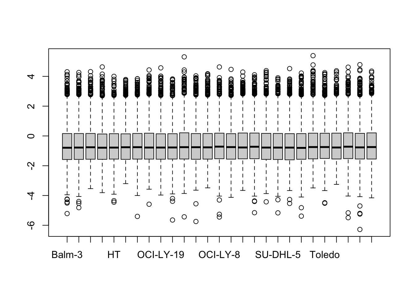

#protNorm <- protData
#assay(protNorm) <- protMatNorm

Create assay experiment object

protTab <- protMatNorm %>% as_tibble(rownames = "uniprotID") %>%
  pivot_longer(-uniprotID, names_to = "Name", values_to = "count") %>%
  left_join(aucTab, by = "Name") %>%
  mutate(symbol = uniprotID, cellLine = Name) %>%
  filter(!symbol %in% c("",NA), !is.na(auc))

protSub <- jyluMisc::tidyToSum(protTab, rowID = "uniprotID",colID = "Name", 
                     values = "count", annoRow = "symbol", annoCol = c("auc","TP53","Subtype","cellLine"))

Identify proteins differentially expressed

Prefilter proteins that did not change

sds <- genefilter::rowSds(assay(protSub))
protSub <- protSub[sds > genefilter::shorth(sds),]
dim(protSub)

[1] 3268   27

Differential protein expression using proDA

protMat <- assay(protSub)
omicList[["protein"]] <- protMat
fit <- proDA(protMat, design = ~ auc,
             col_data = colData(protSub))

resTab <- test_diff(fit, contrast = "auc") %>%
  arrange(pval) %>%
  mutate(symbol = rowData(protSub[name,])$symbol)

resTab.base.embl <- resTab

hist(resTab$pval)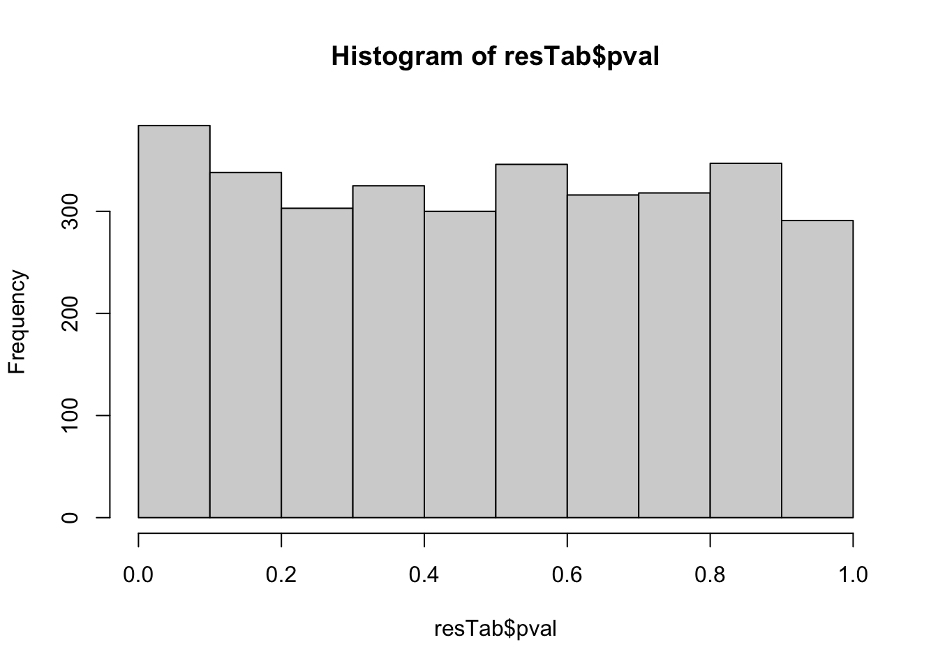

Stronger associations can be observed

Proteins with p-value < 0.05

resTab.sig <- filter(resTab, pval < 0.05)
resTab.sig %>% select(symbol, pval, adj_pval, diff) %>%
  mutate_if(is.numeric, formatC, digits=1) %>%
  DT::datatable()

Plot top 9 examples

pList <- lapply(seq(9), function(i) {
  rec <- resTab.sig[i,]
  plotTab <- tibble(expr = protMat[rec$name,],
                    auc = protSub$auc,
                    TP53 = protSub$TP53,
                    Name = colnames(protSub)) 
  ggplot(plotTab, aes(x=auc, y=expr)) +
    geom_point(aes(col = TP53)) +
    ggrepel::geom_text_repel(aes(label = Name)) +
    ggtitle(rec$symbol) +
    geom_smooth(method="lm", se= FALSE) +
    theme_bw()
})

cowplot::plot_grid(plotlist = pList,ncol=3)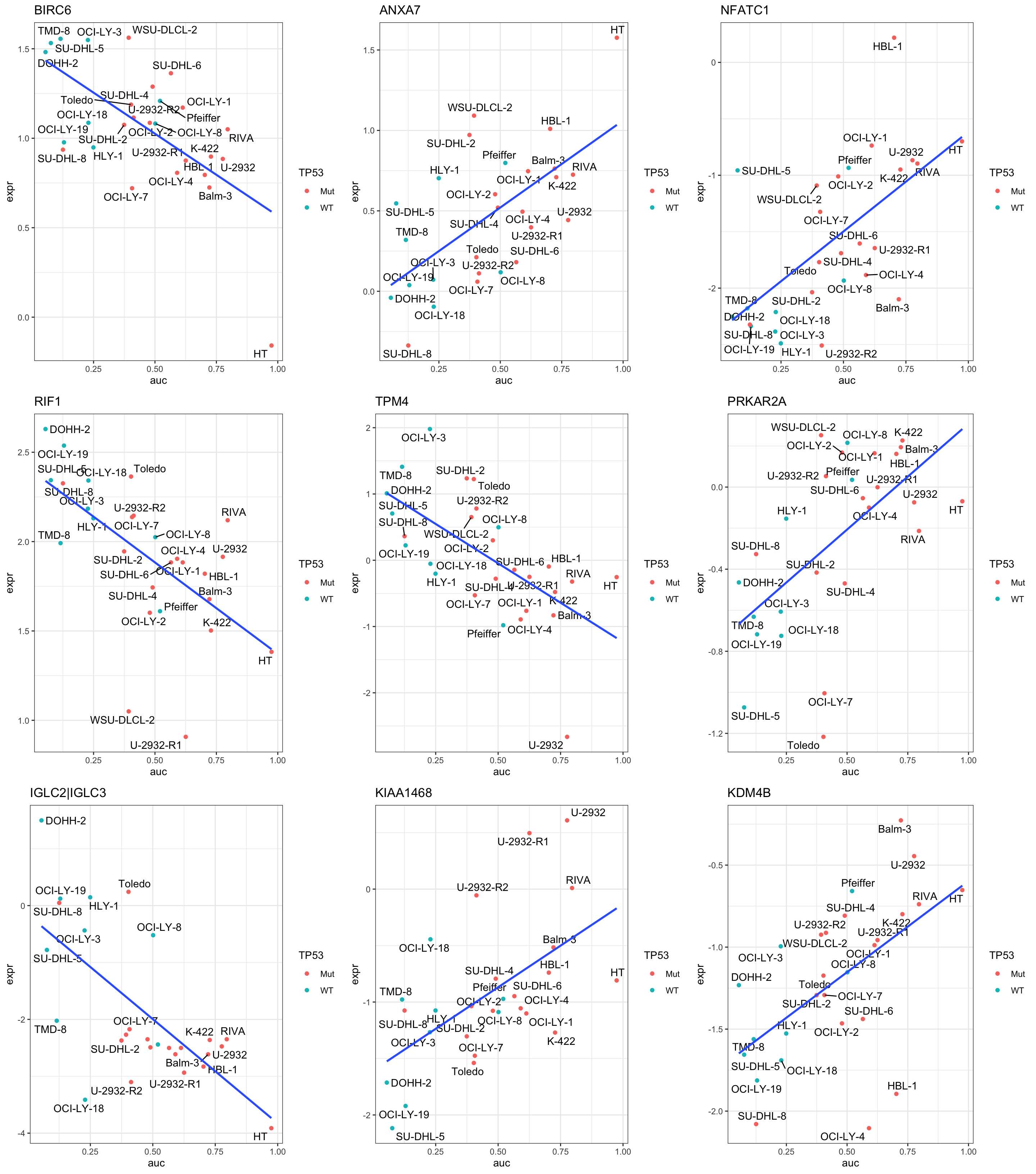

Enrichment analysis

gmts = list(H= "../data/gmts/h.all.v6.2.symbols.gmt",
            KEGG = "../data/gmts/c2.cp.kegg.v6.2.symbols.gmt",
            C6 = "../data/gmts/c6.all.v6.2.symbols.gmt")
inputTab <- resTab %>% filter(pval < 0.1) %>%
  distinct(symbol, .keep_all = TRUE) %>%
  select(symbol, t_statistic) %>% data.frame() %>% column_to_rownames("symbol")
enRes <- list()
enRes[["Hallmark"]] <- runGSEA(inputTab, gmts$H, "page")
enRes[["KEGG"]] <- runGSEA(inputTab, gmts$KEGG,"page")
enRes[["Perturbation"]] <- runGSEA(inputTab, gmts$C6,"page")
p <- plotEnrichmentBar(enRes, pCut =0.05, ifFDR= FALSE)
cowplot::plot_grid(p)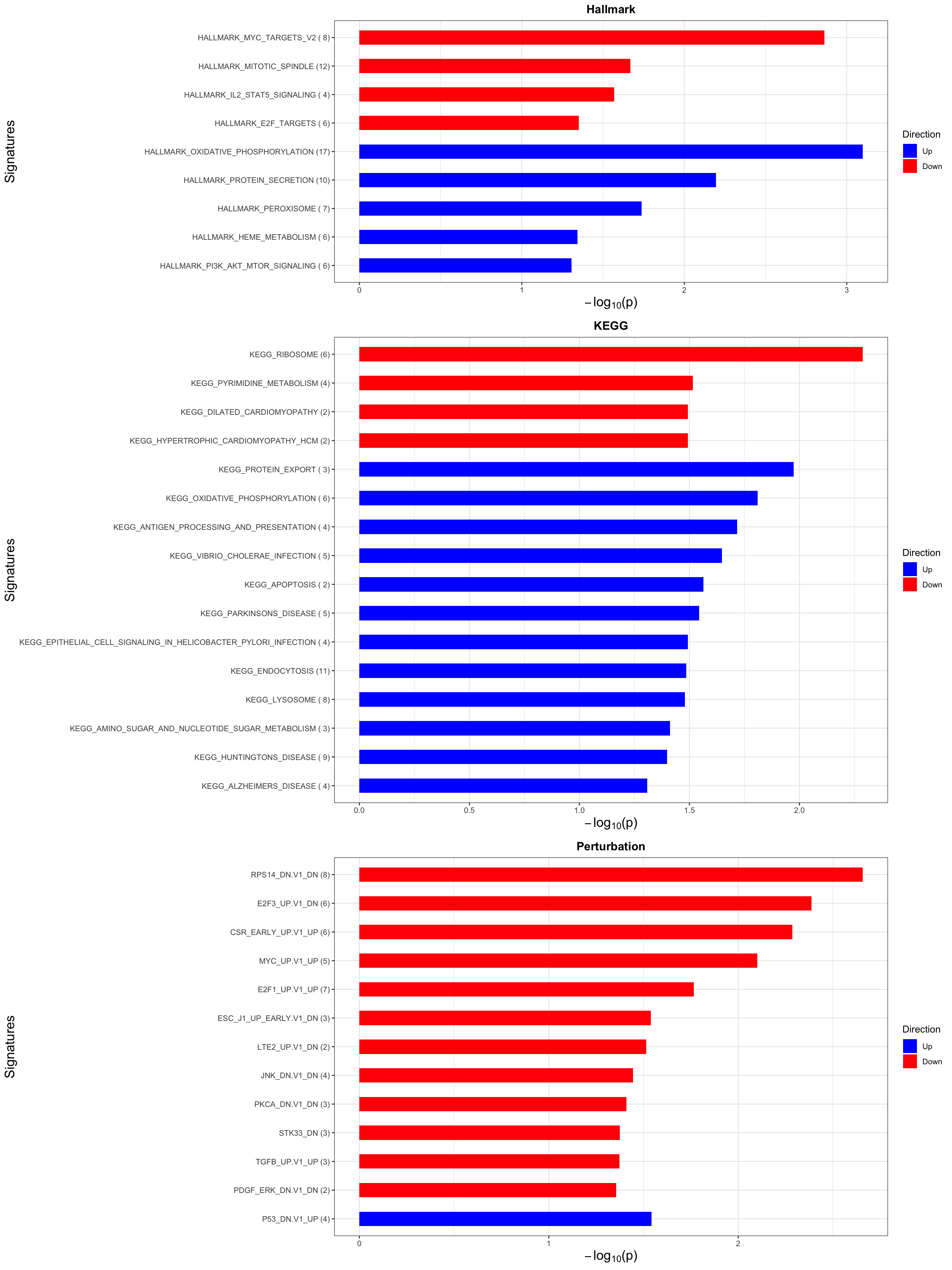

Focus on proteins from Fatty acid metabolism pathway

geneList <- piano::loadGSC(gmts$H)$gsc$HALLMARK_FATTY_ACID_METABOLISM
plotGene <- filter(filter(resTab, pval <= 0.05), symbol%in% geneList )

pList <- lapply(seq(nrow(plotGene)), function(i) {
  rec <- plotGene[i,]
  plotTab <- tibble(expr = protMat[rec$name,],
                    auc = protSub$auc,
                    TP53 = protSub$TP53,
                    Name = colnames(protSub)) 
  ggplot(plotTab, aes(x=auc, y=expr)) +
    geom_point(aes(col = TP53)) +
    ggrepel::geom_text_repel(aes(label = Name)) +
    ggtitle(rec$symbol) +
    geom_smooth(method="lm", se= FALSE) +
    theme_bw()
})

cowplot::plot_grid(plotlist = pList,ncol=3)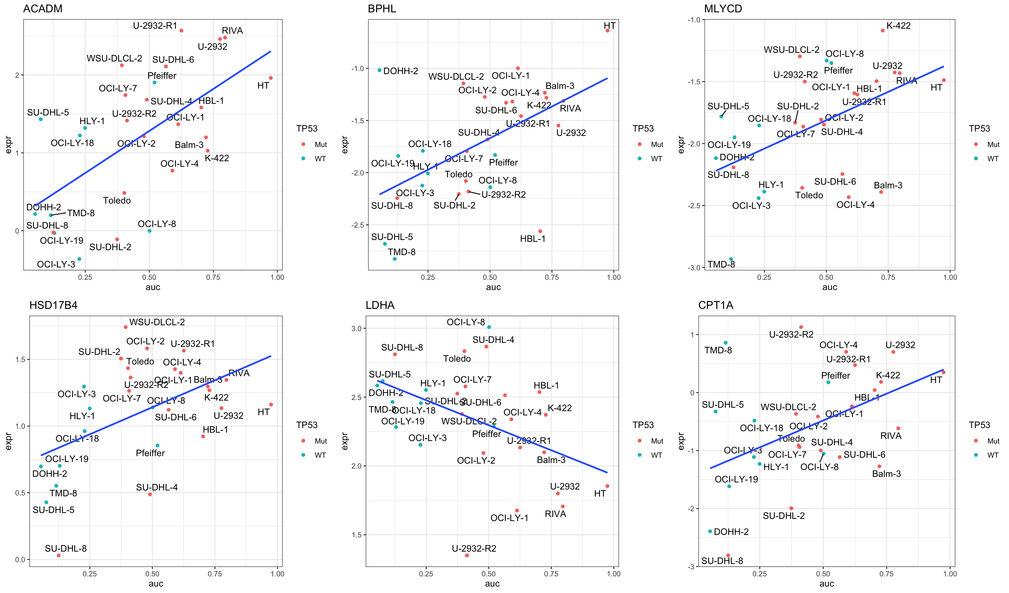

Metabolimics

Process metabolomic data

Normalization (not performed)

metaData <- readRDS("../data/SC005_SummarizedExperiment_metabolomics.RDS")
metaData <- metaData[,metaData$cell.line %in% aucTab$Name & metaData$condition =="U"]
metaMat <- assay(metaData)
boxplot(metaMat)

#metaMatNorm <- PhosR::medianScaling(metaMat, scale = FALSE)
metaMatNorm <- metaMat
boxplot(metaMatNorm)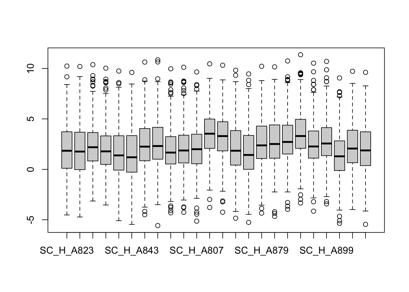

metaNorm <- metaData
assay(metaNorm) <- metaMatNorm
assayNames(metaNorm) <- "norm"

Average technical replicates for each cell line

metaTab <- jyluMisc::sumToTidy(metaNorm) %>%
  group_by(cell.line, rowID, metabolite, class, condition) %>%
  summarise(count = mean(norm, na.rm=TRUE)) %>%
  dplyr::rename(symbol = metabolite, cellLine = cell.line) %>%
  mutate(colID = paste0(cellLine,"_", condition)) %>%
  ungroup()

metaSub <- jyluMisc::tidyToSum(metaTab, rowID = "rowID", colID = "colID", 
                     values = "count", annoRow = "symbol", 
                     annoCol = c("condition", "cellLine"))

#add additional annotations
metaSub$auc <- aucTab[match(metaSub$cellLine, aucTab$Name),]$auc
metaSub$TP53 <- aucTab[match(metaSub$cellLine, aucTab$Name),]$TP53
metaSub$Subtype <- aucTab[match(metaSub$cellLine, aucTab$Name),]$Subtype
#remove uncessary samples and records
metaSub <- metaSub[!rowData(metaSub)$symbol %in% c("",NA), !is.na(metaSub$auc)]
dim(metaSub)

[1] 286  12

colData(metaSub) %>% data.frame() %>% DT::datatable()

Differential metabolites abundance

metaMat <- assay(metaSub)
omicList[["metabolite"]] <- metaMat
designMat <- model.matrix(~ metaSub$auc)
fit <- lmFit(metaMat, designMat)
fit2 <- eBayes(fit)

resTab <- topTable(fit2, number= Inf, coef= "metaSub$auc") %>%
  dplyr::rename(pval = P.Value, adj_pval = adj.P.Val) %>%
  arrange(pval) %>%
  as_tibble(rownames = "name") %>%
  mutate(symbol = rowData(metaSub[name,])$symbol)

hist(resTab$pval)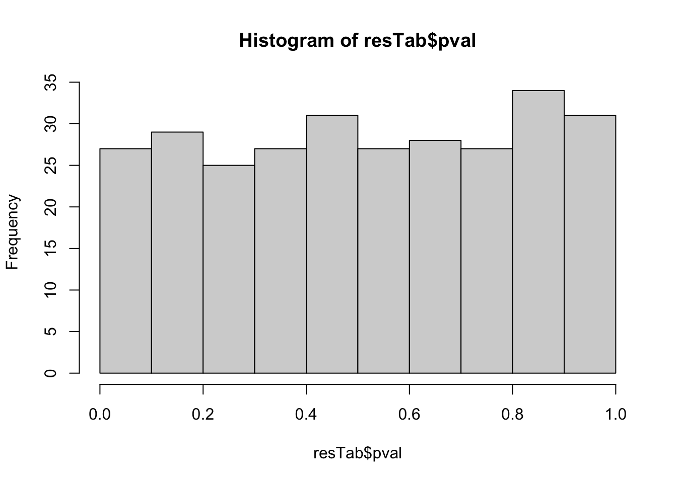

Not strong difference

metabolites with p-value < 0.05

resTab.sig <- filter(resTab, pval < 0.05)
resTab.sig %>% select(symbol, pval, adj_pval, logFC, t) %>%
  mutate_if(is.numeric, formatC, digits=1) %>%
  DT::datatable()

Plot top 9 examples

pList <- lapply(seq(9), function(i) {
  rec <- resTab.sig[i,]
  plotTab <- tibble(expr = metaMat[rec$name,],
                    auc = metaSub$auc,
                    TP53 = metaSub$TP53,
                    Name = colnames(metaSub)) 
  ggplot(plotTab, aes(x=auc, y=expr)) +
    geom_point(aes(col = TP53)) +
    ggrepel::geom_text_repel(aes(label = Name)) +
    ggtitle(rec$symbol) +
    geom_smooth(method="lm", se= FALSE) +
    theme_bw()
})

cowplot::plot_grid(plotlist = pList,ncol=3)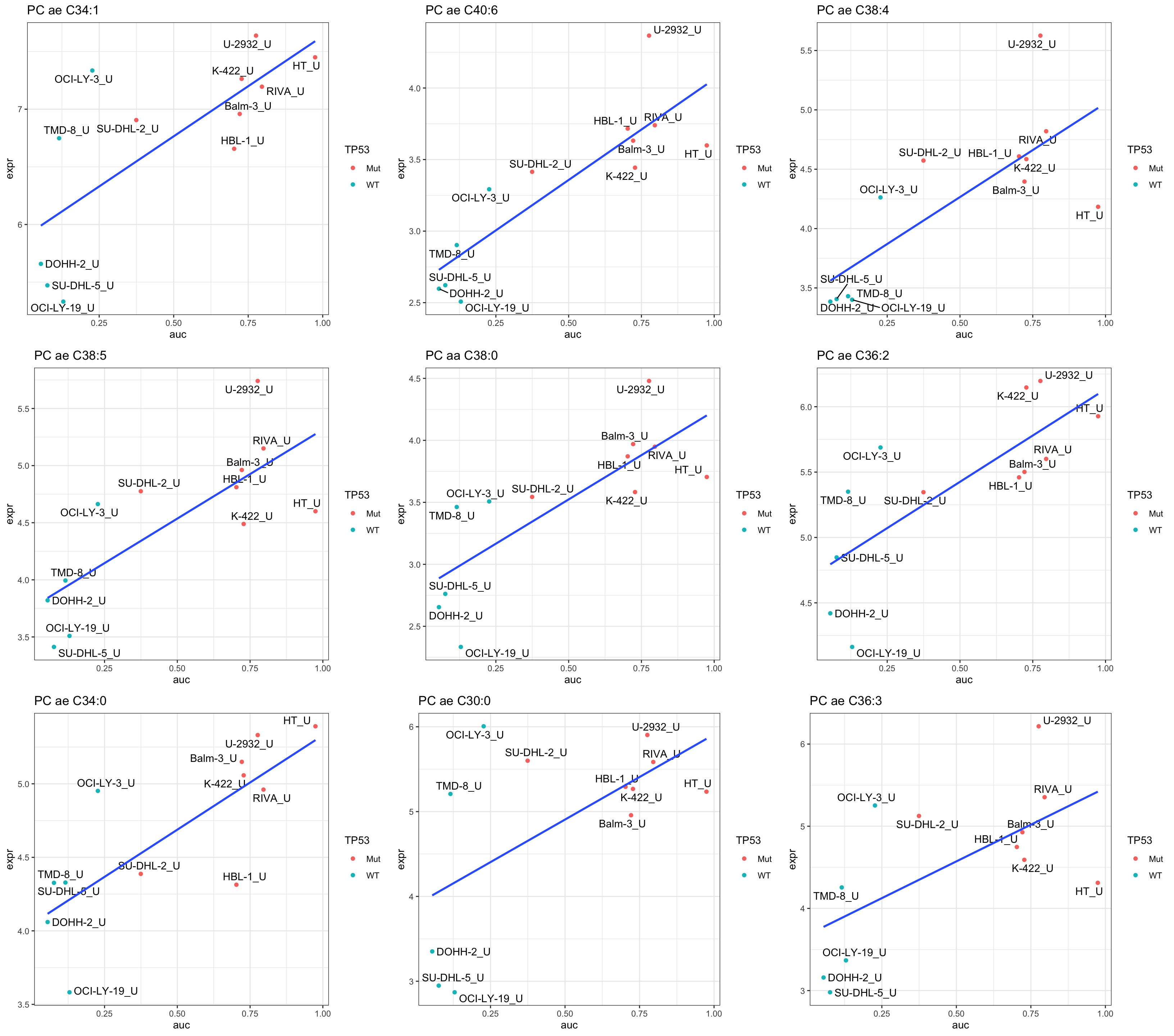

Differential gene expression analysis based on public data

Proprocessing

load("../data/DepMap_GEXwide.RData")
exprMat <- t(DepMap_GEXwide)
exprMat <- exprMat[,colnames(exprMat) %in% aucTab$Name]

# Remove low count genes
exprMat <- exprMat[rowMedians(exprMat) >0,]

dim(exprMat)

[1] 15654    14

boxplot(exprMat)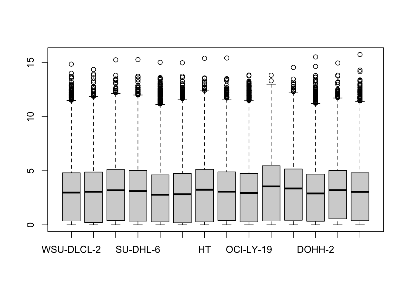

vstObj <- vsn::vsnMatrix(exprMat)
#exprMat <- vsn::predict(vstObj, exprMat)

#boxplot(exprMat)

#save process data
#save(exprMat, file = "gene_exprMat.RData")

Invariance filtering

sds <- genefilter::rowSds(exprMat)
exprMat <- exprMat[sds > genefilter::shorth(sds),]
dim(exprMat)

[1] 8392   14

omicList[["rna"]] <- exprMat

Differential expression using limma

colTab <- aucTab[match(colnames(exprMat), aucTab$Name),] %>%
  column_to_rownames("Name") %>% data.frame()
designMat <- model.matrix(~auc, colTab)

fit <- lmFit(exprMat, designMat)
fit2 <- eBayes(fit)
resTab <- topTable(fit2, number = Inf, coef = "auc") %>%
  as_tibble(rownames = "symbol")
hist(resTab$P.Value)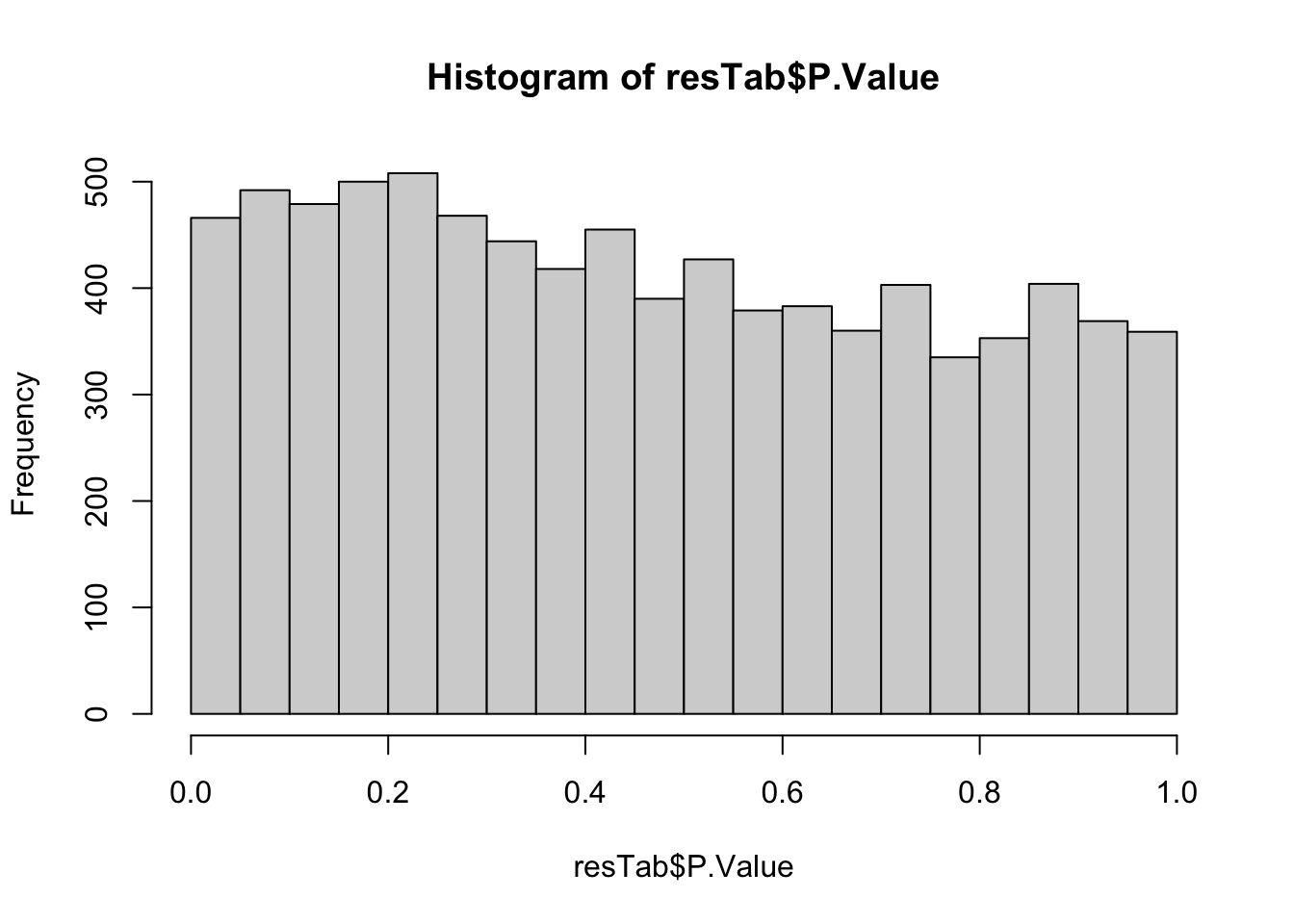

Associations with p <= 0.05

resTab.sig <- filter(resTab, P.Value <= 0.05)
resTab.sig %>% mutate_if(is.numeric, formatC, digits=2) %>% DT::datatable()

Plot top 9 examples

pList <- lapply(seq(9), function(i) {
  rec <- resTab.sig[i,]
  
  plotTab <- tibble(expr = exprMat[rec$symbol,],
                    auc = colTab$auc,
                    TP53 = colTab$TP53,
                    Name = colnames(exprMat)) 
  ggplot(plotTab, aes(x=auc, y=expr)) +
    geom_point(aes(col = TP53)) +
    ggrepel::geom_text_repel(aes(label = Name)) +
    ggtitle(rec$symbol) +
    geom_smooth(method="lm", se= FALSE) +
    theme_bw()
})

cowplot::plot_grid(plotlist = pList,ncol=3)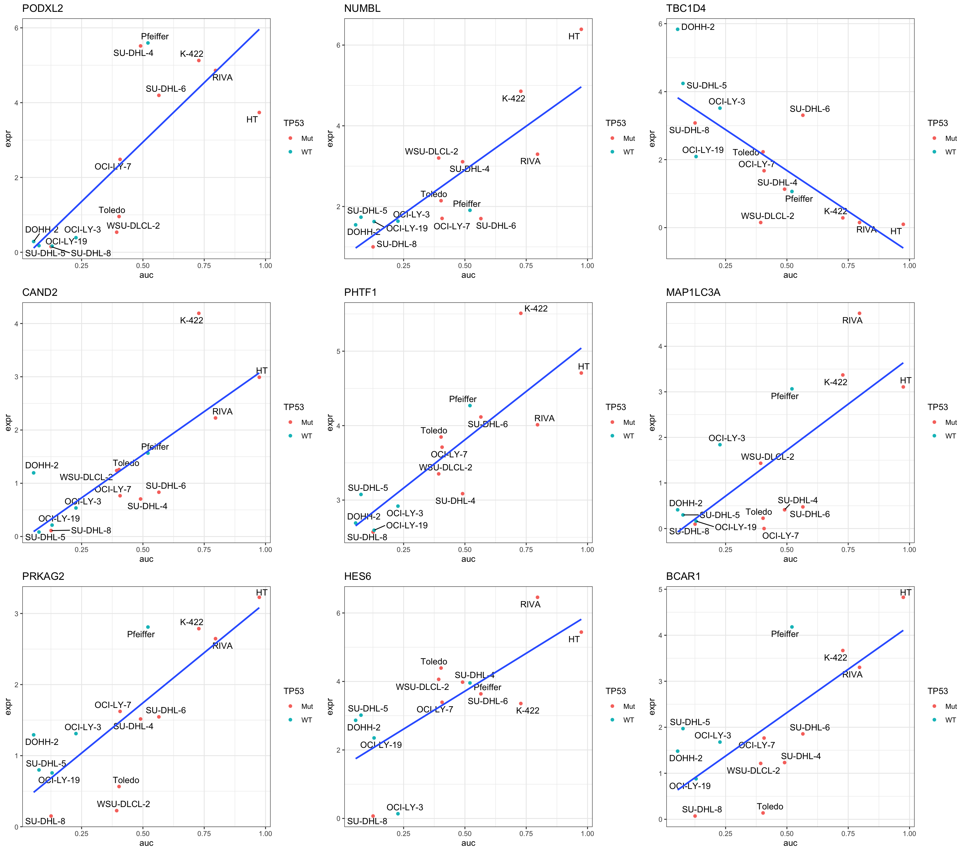

Enrichment analysis

gmts = list(H= "../data/gmts/h.all.v6.2.symbols.gmt",
            KEGG = "../data/gmts/c2.cp.kegg.v6.2.symbols.gmt",
            C6 = "../data/gmts/c6.all.v6.2.symbols.gmt")
inputTab <- resTab %>% filter(P.Value < 0.1) %>%
  distinct(symbol, .keep_all = TRUE) %>%
  select(symbol, t) %>% data.frame() %>% column_to_rownames("symbol")
enRes <- list()
enRes[["Hallmark"]] <- runGSEA(inputTab, gmts$H, "page")
enRes[["KEGG"]] <- runGSEA(inputTab, gmts$KEGG,"page")
enRes[["Perturbation"]] <- runGSEA(inputTab, gmts$C6,"page")
p <- plotEnrichmentBar(enRes, pCut =0.01, ifFDR= FALSE)
cowplot::plot_grid(p)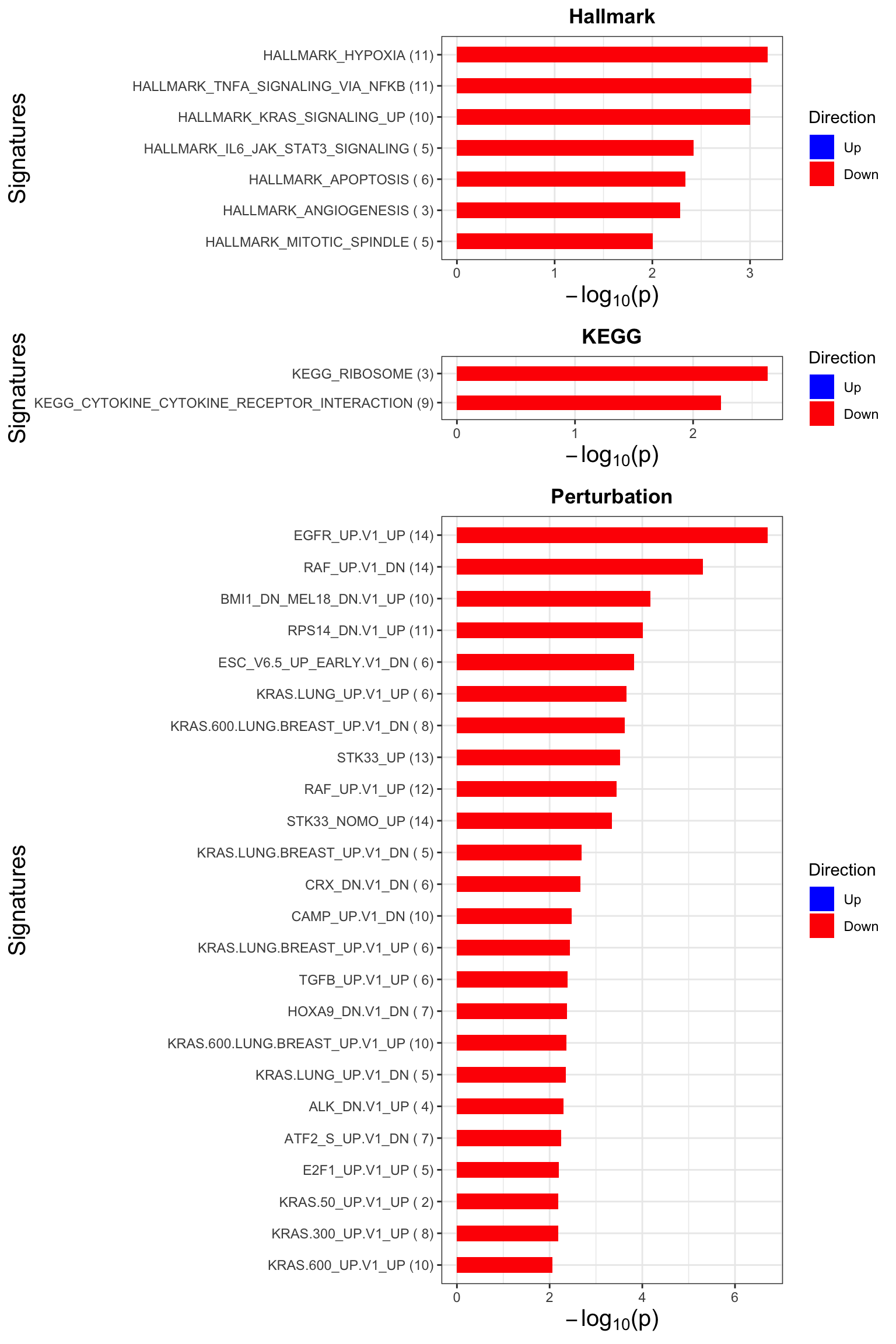

Focus on proteins from Fatty acid metabolism pathway

geneList <- piano::loadGSC(gmts$H)$gsc$HALLMARK_FATTY_ACID_METABOLISM
plotGene <- filter(filter(resTab, P.Value <= 0.05), symbol%in% geneList )
pList <- lapply(seq(nrow(plotGene)), function(i) {
  rec <- plotGene[i,]
  plotTab <- tibble(expr = exprMat[rec$symbol,],
                    auc = colTab$auc,
                    TP53 = colTab$TP53,
                    Name = colnames(exprMat)) 
  ggplot(plotTab, aes(x=auc, y=expr)) +
    geom_point(aes(col = TP53)) +
    ggrepel::geom_text_repel(aes(label = Name)) +
    ggtitle(rec$symbol) +
    geom_smooth(method="lm", se= FALSE) +
    theme_bw()
})

cowplot::plot_grid(plotlist = pList,ncol=3)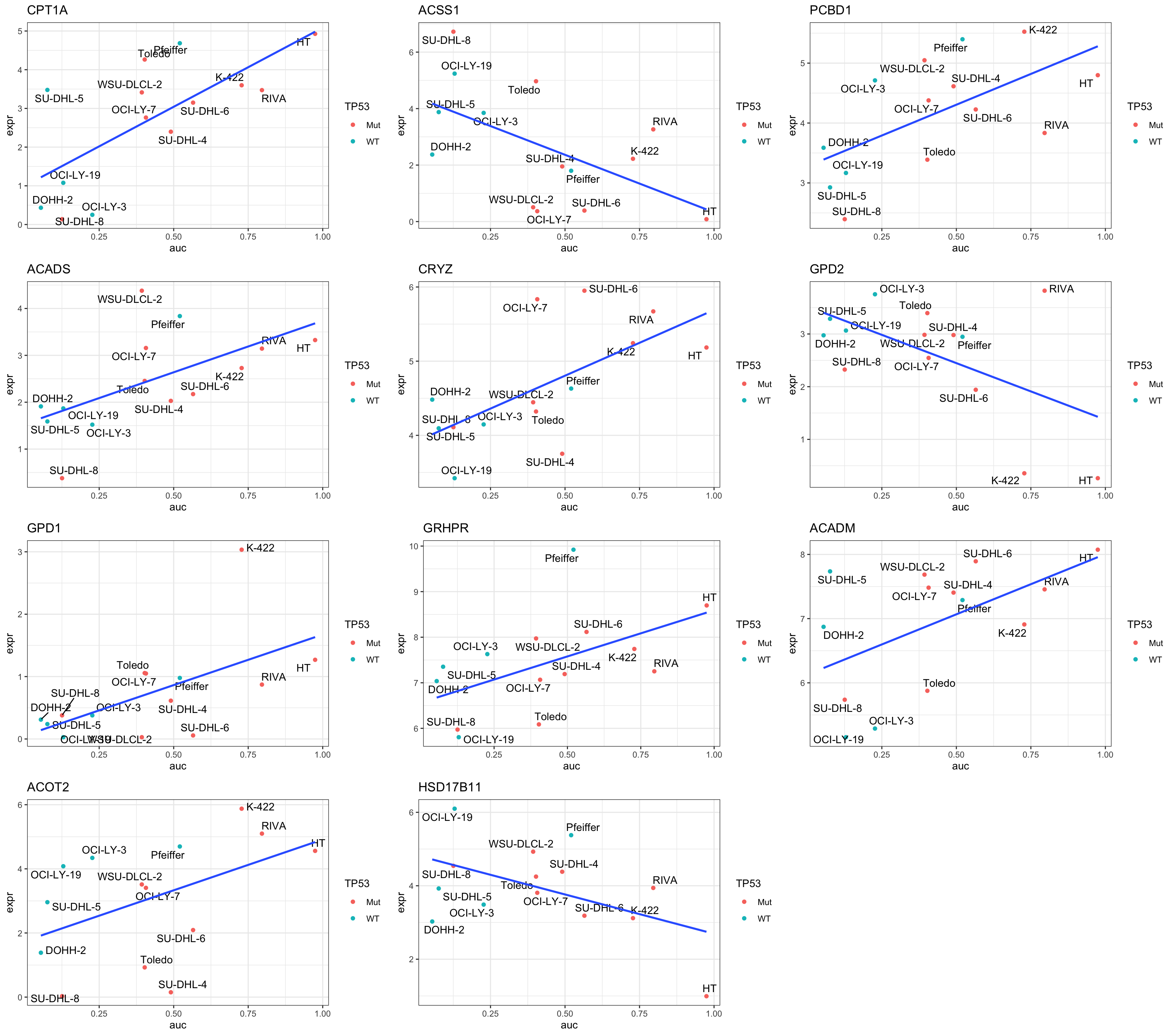

MOFA analysis

library(MOFA2)

Preprocessing

mofaData <- omicList

Only use top 5000 most variant rna expression

exprMat <- mofaData$rna
sds <- genefilter::rowSds(exprMat)
exprMat <- exprMat[order(sds, decreasing = TRUE)[1:5000],]
mofaData$rna <- exprMat

Change column names of the metabolite matrix

colnames(mofaData$metabolite) <- str_remove(colnames(mofaData$metabolite),"_U")

Create MOFA object

# Create MultiAssayExperiment object 
mofaData <- MultiAssayExperiment::MultiAssayExperiment(
  experiments = mofaData
)

MOFAobject <- create_mofa_from_MultiAssayExperiment(mofaData)

Plot data overview

plot_data_overview(MOFAobject)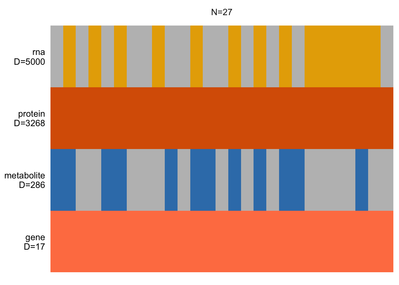

Define MOFA options

Data options

data_opts <- get_default_data_options(MOFAobject)
data_opts

$scale_views
[1] FALSE

$scale_groups
[1] FALSE

$center_groups
[1] TRUE

$use_float32
[1] FALSE

$views
[1] "gene"       "protein"    "metabolite" "rna"       

$groups
[1] "group1"

Model options

model_opts <- get_default_model_options(MOFAobject)
model_opts$num_factors <- 10

model_opts

$likelihoods
      gene    protein metabolite        rna 
"gaussian" "gaussian" "gaussian" "gaussian" 

$num_factors
[1] 10

$spikeslab_factors
[1] FALSE

$spikeslab_weights
[1] TRUE

$ard_factors
[1] FALSE

$ard_weights
[1] TRUE

Change the likely hood of Mutations to “bernoulli

model_opts$likelihoods[["gene"]] <- "bernoulli"
model_opts$likelihoods

       gene     protein  metabolite         rna 
"bernoulli"  "gaussian"  "gaussian"  "gaussian"

Training options

train_opts <- get_default_training_options(MOFAobject)
train_opts$convergence_mode <- "slow"
train_opts$seed <- 2022
train_opts$maxiter <- 10000
train_opts

$maxiter
[1] 10000

$convergence_mode
[1] "slow"

$drop_factor_threshold
[1] -1

$verbose
[1] FALSE

$startELBO
[1] 1

$freqELBO
[1] 5

$stochastic
[1] FALSE

$gpu_mode
[1] FALSE

$seed
[1] 2022

$outfile
NULL

$weight_views
[1] FALSE

$save_interrupted
[1] FALSE

Change drop threshold to 0.01

train_opts$drop_factor_threshold <-0.01

Train the MOFA model

Prepare MOFA object

MOFAobject <- prepare_mofa(MOFAobject,
  data_options = data_opts,
  model_options = model_opts,
  training_options = train_opts
)

Training

MOFAobject <- run_mofa(MOFAobject)
saveRDS(MOFAobject,"../output/mofaDLBCL_Doxo.rds")

Preliminary analysis of the results

MOFAobject <- readRDS("../output/mofaDLBCL_Doxo.rds")

Factor correlation matrix

plot_factor_cor(MOFAobject)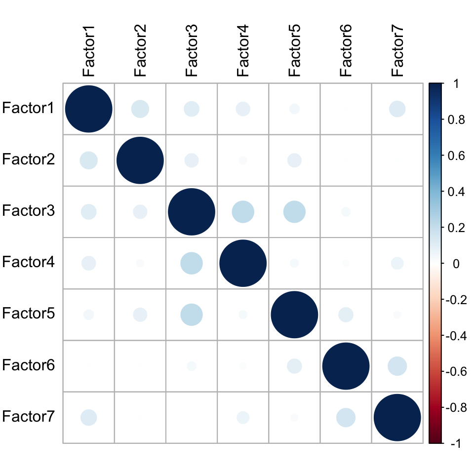

Variance explained

plot_variance_explained(MOFAobject, max_r2=15)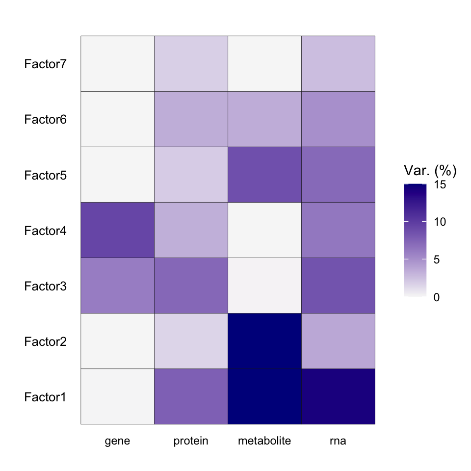

Total variance explained

plot_variance_explained(MOFAobject, plot_total = T)[[2]]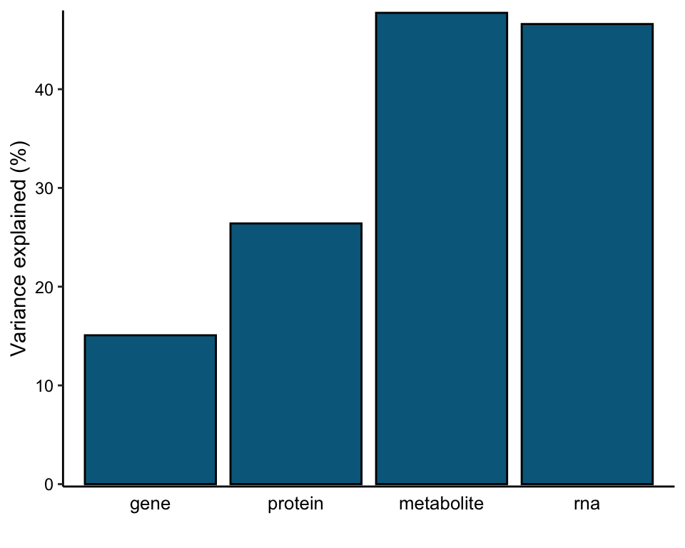

Factor heatmap

library(pheatmap)
#gene annotation
facMat <- t(get_factors(MOFAobject)[[1]])

colAnno <- aucTab %>% column_to_rownames("Name")

pheatmap(facMat, clustering_method = "ward.D2", annotation_col = colAnno)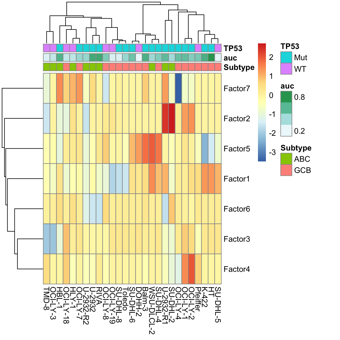

Correlation between factors and annotations

facTab <- facMat %>% as_tibble(rownames = "factor") %>%
  pivot_longer(-factor, names_to = "Name", values_to = "value") %>%
  left_join(aucTab, by= "Name")

Subtype

resTab <- facTab %>% group_by(factor) %>% nest() %>%
  mutate(m=map(data, ~t.test(value ~ Subtype,.))) %>%
  mutate(res = map(m, broom::tidy)) %>%
  unnest(res) %>%
  select(factor, estimate, p.value) %>% 
  arrange(p.value)
head(resTab)

# A tibble: 6 × 3
# Groups:   factor [6]
  factor  estimate p.value
  <chr>      <dbl>   <dbl>
1 Factor3   -0.957 0.00518
2 Factor4   -0.380 0.100  
3 Factor6   -0.555 0.112  
4 Factor7    0.443 0.244  
5 Factor5   -0.204 0.588  
6 Factor1   -0.117 0.743

ggplot(filter(facTab, factor == "Factor3"), aes(x=Subtype, y=value)) +
  geom_boxplot() + geom_point()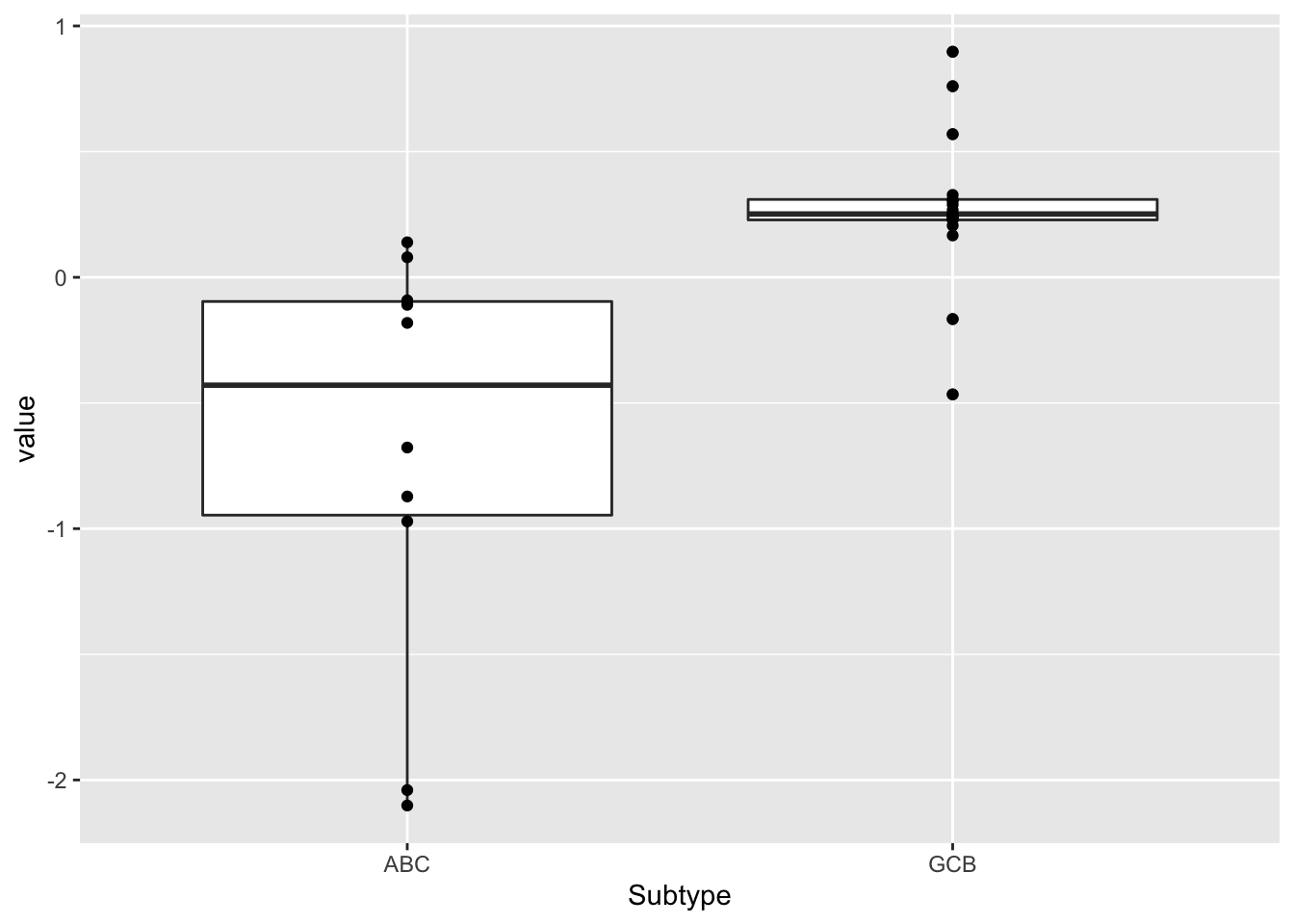

TP55

resTab <- facTab %>% group_by(factor) %>% nest() %>%
  mutate(m=map(data, ~t.test(value ~ TP53,.))) %>%
  mutate(res = map(m, broom::tidy)) %>%
  unnest(res) %>%
  select(factor, estimate, p.value) %>% 
  arrange(p.value)
head(resTab)

# A tibble: 6 × 3
# Groups:   factor [6]
  factor  estimate p.value
  <chr>      <dbl>   <dbl>
1 Factor6  -0.382   0.0594
2 Factor2   0.477   0.164 
3 Factor1   0.484   0.201 
4 Factor3   0.371   0.339 
5 Factor4  -0.149   0.528 
6 Factor7   0.0648  0.860

ggplot(filter(facTab, factor == "Factor6"), aes(x=TP53, y=value)) +
  geom_boxplot() + geom_point()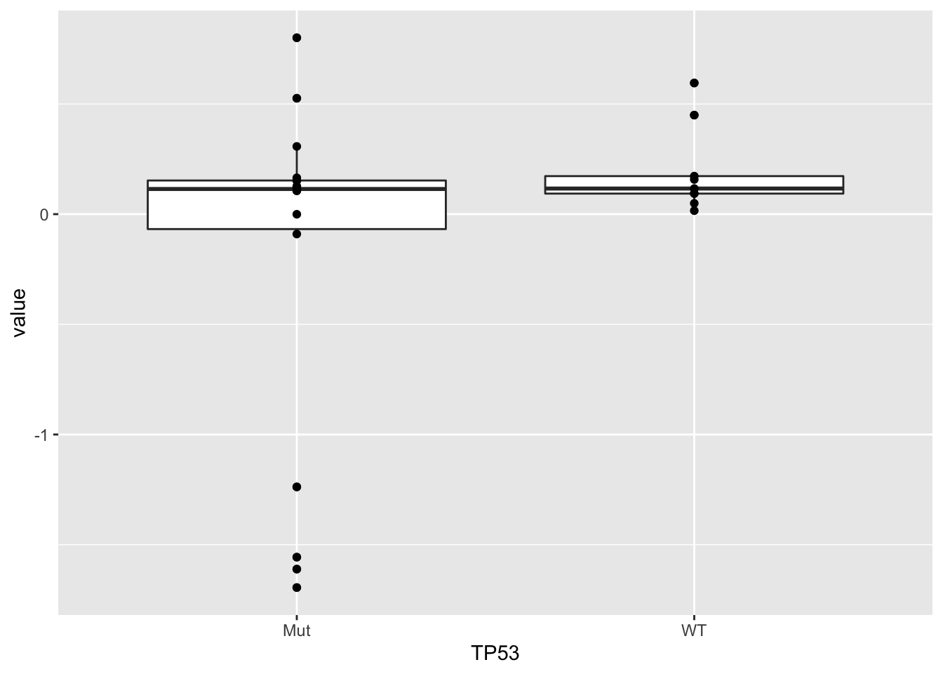

Doxorubicin response

resTab <- facTab %>% group_by(factor) %>% nest() %>%
  mutate(m=map(data, ~cor.test(~ value + auc,.))) %>%
  mutate(res = map(m, broom::tidy)) %>%
  unnest(res) %>%
  select(factor, estimate, p.value) %>% 
  arrange(p.value)
head(resTab)

# A tibble: 6 × 3
# Groups:   factor [6]
  factor  estimate p.value
  <chr>      <dbl>   <dbl>
1 Factor1   0.430   0.0251
2 Factor6  -0.311   0.114 
3 Factor5  -0.170   0.397 
4 Factor2   0.136   0.500 
5 Factor3   0.127   0.529 
6 Factor4  -0.0588  0.771

ggplot(filter(facTab, factor == "Factor1"), aes(x=auc, y=value)) +
  geom_point(aes(col = TP53)) + 
  geom_smooth(method = "lm") +
  ggrepel::geom_text_repel(aes(label = Name))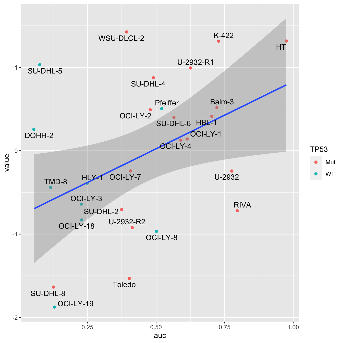

Focus on F1 (Doxorubicine response)

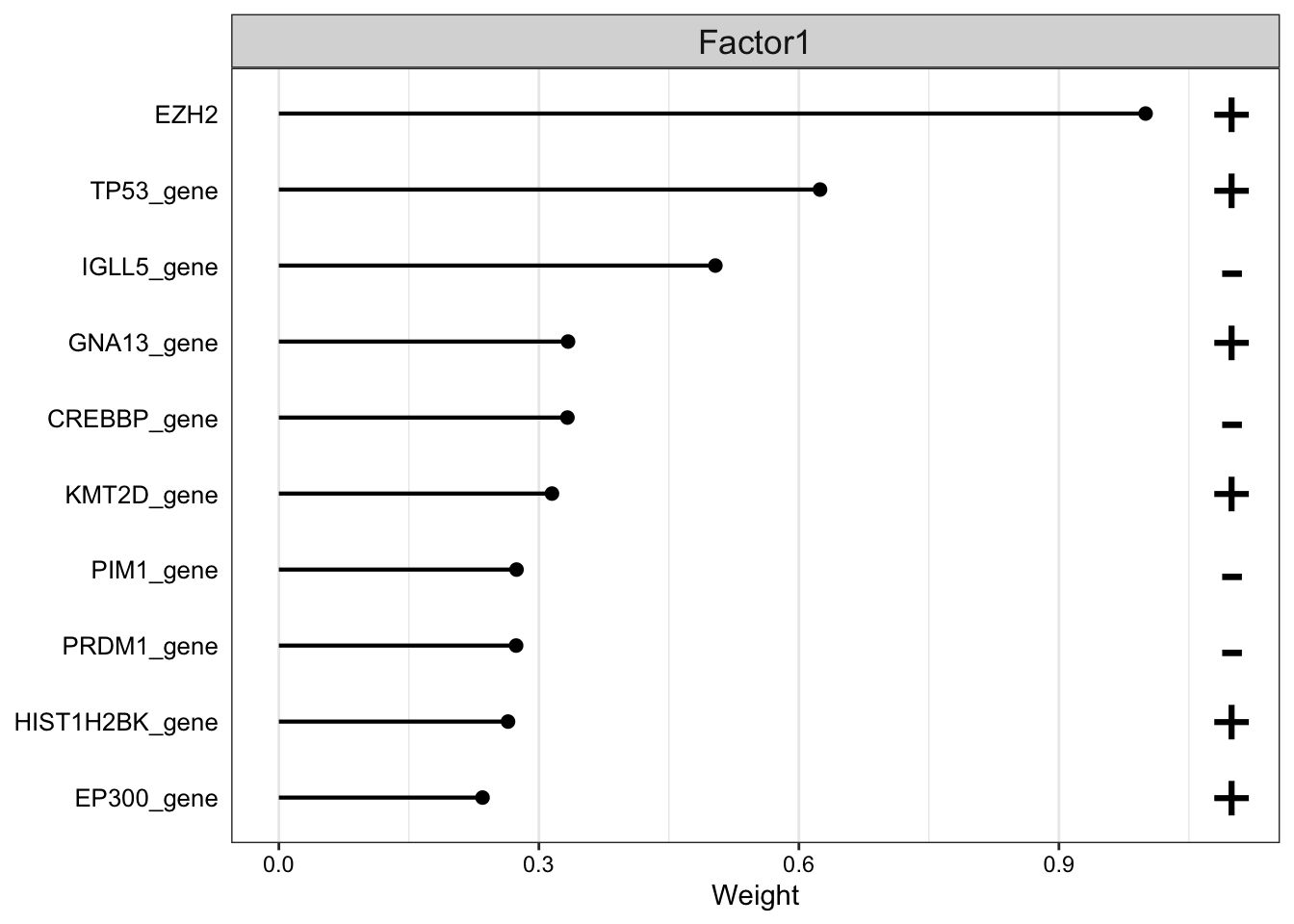
Weight of genomic features

plot_top_weights(MOFAobject,
 view = "gene",
 factor = 1,
 nfeatures = 10,     # Top number of features to highlight
 scale = T           # Scale weights from -1 to 1
)

F1 values versus TP53 mutation

plot_factor(MOFAobject, 
  factors = 1, 
  color_by = "TP53_gene",
  add_violin = TRUE,
  dodge = TRUE
)

F1 values versus EZH2 mutation

plot_factor(MOFAobject, 
  factors = 1, 
  color_by = "EZH2",
  add_violin = TRUE,
  dodge = TRUE
)

Weight of protein features

plot_top_weights(MOFAobject,
 view = "protein",
 factor = 1,
 nfeatures = 10,     # Top number of features to highlight
 scale = T           # Scale weights from -1 to 1
)

Weight of rna features

plot_top_weights(MOFAobject,
 view = "rna",
 factor = 1,
 nfeatures = 10,     # Top number of features to highlight
 scale = T           # Scale weights from -1 to 1
)

Weight of metabolites features

plot_top_weights(MOFAobject,
 view = "metabolite",
 factor = 1,
 nfeatures = 10,     # Top number of features to highlight
 scale = T           # Scale weights from -1 to 1
)

Focus on F3 (Subtype)

Weight of genomic features on LF3

plot_top_weights(MOFAobject,
 view = "gene",
 factor =3,
 nfeatures = 10,     # Top number of features to highlight
 scale = T           # Scale weights from -1 to 1
)

Weight of protein features on LF3

plot_top_weights(MOFAobject,
 view = "protein",
 factor =3,
 nfeatures = 10,     # Top number of features to highlight
 scale = T           # Scale weights from -1 to 1
)

Weight of rna features on LF3

plot_top_weights(MOFAobject,
 view = "rna",
 factor =3,
 nfeatures = 10,     # Top number of features to highlight
 scale = T           # Scale weights from -1 to 1
)

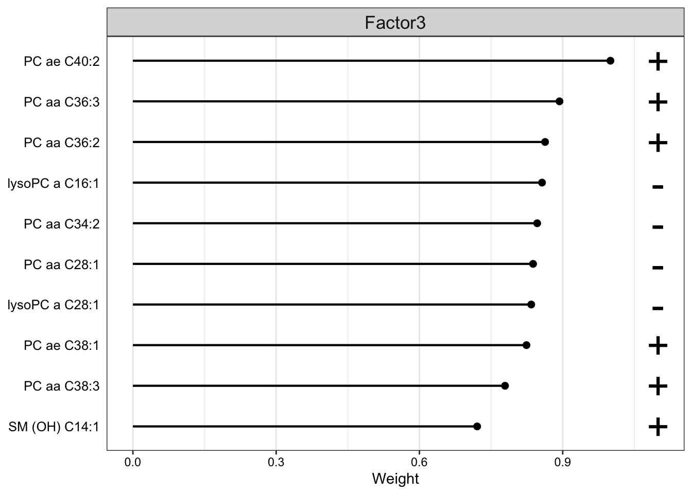
Weight of metabolite features on LF3

plot_top_weights(MOFAobject,
 view = "metabolite",
 factor =3,
 nfeatures = 10,     # Top number of features to highlight
 scale = T           # Scale weights from -1 to 1
)

LASSO regression for predicting Doxorubicine responses

library(glmnet)
detach(package:MOFA2, unload = TRUE)

Preprocessing data

Response vector

responseList <- list(Doxorubicin = structure(aucTab$auc, names=aucTab$Name))

RNAseq data

lassoData <- omicList
exprMat <- lassoData$rna
sds <- genefilter::rowSds(exprMat)
exprMat <- exprMat[order(sds, decreasing = TRUE)[1:5000],]
exprMat <- t(exprMat)
colnames(exprMat) <- paste0(colnames(exprMat),"_rna")

Proteomic data

protMat <- t(lassoData$protein)
colnames(protMat) <- paste0(colnames(protMat),"_protein")

Genomic data

geneMat <- t(lassoData$gene)
colnames(geneMat) <- paste0(colnames(geneMat),"_gene")

Metabolomic data

metaMat <- lassoData$metabolite
colnames(metaMat) <- str_remove(colnames(metaMat),"_U")
metaMat <- t(metaMat)
colnames(metaMat) <- paste0(colnames(metaMat),"_metabolite")

Feature selection with LASSO penalty

#Functions for running glm
runGlm <- function(X, y, method = "ridge", repeats=20, folds = 3, lambda = "lambda.min") {
  modelList <- list()
  lambdaList <- c()
  varExplain <- c()
  coefMat <- matrix(NA, ncol(X), repeats)
  rownames(coefMat) <- colnames(X)

  if (method == "lasso"){
    alpha = 1
  } else if (method == "ridge") {
    alpha = 0
  }
  
  for (i in seq(repeats)) {
    if (ncol(X) > 2) {
      res <- cv.glmnet(X,y, type.measure = "mse", family="gaussian", 
                       nfolds = folds, alpha = alpha, standardize = FALSE)
      lambdaList <- c(lambdaList, res[[lambda]])
      modelList[[i]] <- res
      
      coefModel <- coef(res, s = lambda)[-1] #remove intercept row
      coefMat[,i] <- coefModel
      
      #calculate variance explained
      y.pred <- predict(res, s = lambda, newx = X)
      varExp <- cor(as.vector(y),as.vector(y.pred))^2
      varExplain[i] <- ifelse(is.na(varExp), 0, varExp) 
      
    } else {
      fitlm<-lm(y~., data.frame(X))
      varExp <- summary(fitlm)$r.squared
      varExplain <- c(varExplain, varExp)
      
    }

  }
  list(modelList = modelList, lambdaList = lambdaList, varExplain = varExplain, coefMat = coefMat)
}

#function for scaling predictors
dataScale <- function(x, censor = NULL, robust = FALSE) {
        #function to scale different variables
        if (length(unique(na.omit(x))) <=3){
          #a binary variable, change to -0.5 and 0.5 for 1 and 2
          x - 0.5
        } else {
          if (robust) {
          #continuous variable, centered by median and divied by 2*mad
          mScore <- (x-median(x,na.rm=TRUE))/mad(x,na.rm=TRUE)
            if (!is.null(censor)) {
              mScore[mScore > censor] <- censor
              mScore[mScore < -censor] <- -censor
            }
          mScore/2
          } else {
            mScore <- (x-mean(x,na.rm=TRUE))/(sd(x,na.rm=TRUE))
              if (!is.null(censor)) {
                mScore[mScore > censor] <- censor
                mScore[mScore < -censor] <- -censor
              }
          mScore/2
          }
        }
      }

#function to generate response vector and explainatory variable for each seahorse measurement
generateData <- function(responseList, inclSet,  onlyCombine = FALSE, censor = NULL, robust = FALSE) {
    
    allResponse <- list()
    allExplain <- list()

    for (measure in names(responseList)) {
      y <- responseList[[measure]]
      y <- y[!is.na(y)]
      
      #get overlapped samples for each dataset 
      overSample <- names(y)
      
      for (eachSet in inclSet) {
        overSample <- intersect(overSample,rownames(eachSet))
      }
      
      y <- dataScale(y[overSample], censor = censor, robust = robust)
      
      expTab <- list()
      
      if ("Gene" %in% names(inclSet)) {
        geneTab <- inclSet$Gene[overSample,]
        #at least 3 mutated sample
        geneTab <- geneTab[, colSums(geneTab) >= 3]
        vecName <- sprintf("genetic(%s)", ncol(geneTab))
        expTab[[vecName]] <- apply(geneTab,2,dataScale)
      }
      
      
      if ("RNA" %in% names(inclSet)){
        rnaMat <- inclSet$RNA[overSample, ]
        colnames(rnaMat) <- paste0("con.",colnames(rnaMat), sep = "")
        vecName <- sprintf("RNA(%s)", ncol(rnaMat))
        expTab[[vecName]] <- apply(rnaMat,2,dataScale, censor = censor, robust = robust)
        
      }
      
      if ("Protein" %in% names(inclSet)){
        protMat <- inclSet$Protein[overSample, ]
        colnames(protMat) <- paste0("con.",colnames(protMat), sep = "")
        vecName <- sprintf("Protein(%s)", ncol(protMat))
        expTab[[vecName]] <- apply(protMat,2,dataScale, censor = censor, robust = robust)
        
      }
        
      if ("Metabolite" %in% names(inclSet)){
        metaMat <- inclSet$Metabolite[overSample, ]
        colnames(metaMat) <- paste0("con.",colnames(metaMat), sep = "")
        vecName <- sprintf("Metabolite(%s)", ncol(metaMat))
        expTab[[vecName]] <- apply(metaMat,2,dataScale, censor = censor, robust = robust)
        
      }
      
      if (length(inclSet) > 1) {
        comboTab <- c()
        for (eachSet in names(expTab)){
          comboTab <- cbind(comboTab, expTab[[eachSet]])
        }
        vecName <- sprintf("all(%s)", ncol(comboTab))
        expTab[[vecName]] <- comboTab
      }
      
      allResponse[[measure]] <- y
      allExplain[[measure]] <- expTab
    }
    
  if (onlyCombine) {
    #only return combined results, for feature selection
    allExplain <- lapply(allExplain, function(x) x[length(x)])
  }
    
  return(list(allResponse=allResponse, allExplain=allExplain))

}

italicizeGene <- function(featureNames) {
  geneNameList <- c("SF3B1","NOTCH1","TP53", "DDX3X","MED12", "ATM","BRAF","EGR2")
  specialCase <- "TP53/del17p"
  formatedList <- sapply(featureNames, function(n) {
    if (n %in% geneNameList) {
      sprintf("italic('%s')",n)
    } else if (n == specialCase) {
      sprintf("italic('TP53')~'/del17p'")
    }
    else {
      sprintf("'%s'",n)
    }
  })
  return(formatedList)
}

formatCNV <- function(cnvList) {
  nameCNV <- c(del17p = "del(17)(p13)", del11q = "del(11)(q22.3)", del13q = "del(13)(q14)", trisomy12 = "trisomy 12", trisomy19 = "trisomy 19")
  cnvList <- sapply(cnvList, function(n) {
    if (n %in% names(nameCNV)) {
      n <- nameCNV[n]
    }
    n
  })
  cnvList
}

library(gtable)
lassoPlot <- function(lassoOut, cleanData, freqCut = 1, coefCut = 0.01, 
                      setNumber = "last", legend = TRUE, labSuffix = " response", scaleFac =1) {
  plotList <- list()
  if (setNumber == "last") {
    setNumber <- length(lassoOut[[1]])
  } else {
    setNumber <- setNumber
  }
  for (seaName in names(lassoOut)) {
    #for the barplot on the left of the heatmap
    barValue <- rowMeans(lassoOut[[seaName]][[setNumber]]$coefMat)
    freqValue <- rowMeans(abs(sign(lassoOut[[seaName]][[setNumber]]$coefMat)))
    barValue <- barValue[abs(barValue) >= coefCut & freqValue >= freqCut] # a certain threshold
    barValue <- barValue[order(barValue)]
    if(length(barValue) == 0) {
      plotList[[seaName]] <- NA
      next
    }

    #for the heatmap and scatter plot below the heatmap
    allData <- cleanData$allExplain[[seaName]][[setNumber]]
    seaValue <- cleanData$allResponse[[seaName]]*2 #back to Z-score
    
    tabValue <- allData[, names(barValue),drop=FALSE]
    ord <- order(seaValue)
    seaValue <- seaValue[ord]
    tabValue <- tabValue[ord, ,drop=FALSE]
    sampleIDs <- rownames(tabValue)
    tabValue <- as.tibble(tabValue)
    
    #change scaled binary back to catagorical
    for (eachCol in colnames(tabValue)) {
      if (strsplit(eachCol, split = "[.]")[[1]][1] != "con") {
        tabValue[[eachCol]] <- as.integer(as.factor(tabValue[[eachCol]]))
      }
      else {
        tabValue[[eachCol]] <- tabValue[[eachCol]]*2 #back to Z-score
      }
    }
    
    tabValue$Sample <- sampleIDs
    #Mark different rows for different scaling in heatmap
    matValue <- gather(tabValue, key = "Var",value = "Value", -Sample)
    matValue$Type <- "mut"
    
    #For continuious value
    matValue$Type[grep("con.",matValue$Var)] <- "con"
    
    #for methylation_cluster
    matValue$Type[grep("ConsCluster",matValue$Var)] <- "meth"
    
    #change the scale of the value, let them do not overlap with each other
    matValue[matValue$Type == "mut",]$Value = matValue[matValue$Type == "mut",]$Value + 10
    matValue[matValue$Type == "meth",]$Value = matValue[matValue$Type == "meth",]$Value + 20
    
    
    #color scale for viability
    idx <- matValue$Type == "con"
    
    myCol <- colorRampPalette(c("blue",'white',"red"), 
                   space = "Lab")
    if (sum(idx) != 0) {
      matValue[idx,]$Value = round(matValue[idx,]$Value,digits = 2)
      minViab <- min(matValue[idx,]$Value)
      maxViab <- max(matValue[idx,]$Value)
      limViab <- max(c(abs(minViab), abs(maxViab)))
      scaleSeq1 <- round(seq(-limViab, limViab,0.01), digits=2)
      color4viab <- setNames(myCol(length(scaleSeq1+1)), nm=scaleSeq1)
    } else {
      scaleSeq1 <- round(seq(0,1,0.01), digits=2)
      color4viab <- setNames(myCol(length(scaleSeq1+1)), nm=scaleSeq1)
    }
    

    
    #change continues measurement to discrete measurement
    matValue$Value <- factor(matValue$Value,levels = sort(unique(matValue$Value)))
    
    #change order of heatmap
    names(barValue) <-  gsub("con.", "", names(barValue))
    matValue$Var <- gsub("con.","",matValue$Var)
    matValue$Var <- factor(matValue$Var, levels = names(barValue))
    matValue$Sample <- factor(matValue$Sample, levels = names(seaValue))
    
    matValue <- matValue %>% mutate(varForm = as.character(Var)) %>%
      mutate(varForm = formatCNV(varForm)) %>%
      mutate(varForm = italicizeGene(varForm)) %>%
      arrange(Var) %>% mutate(varForm = factor(varForm, levels = unique(varForm)))
    
    #plot the heatmap
    p1 <- ggplot(matValue, aes(x=Sample, y=Var)) + geom_tile(aes(fill=Value), color = "gray") + 
      theme_bw() +
      scale_y_discrete(expand=c(0,0),position = "right",labels = parse(text = levels(matValue$varForm))) +
      theme(axis.text.y=element_text(hjust=0, size=10*scaleFac), axis.text.x=element_blank(), 
            axis.title = element_blank(),
            axis.ticks=element_blank(), panel.border=element_rect(colour="gainsboro"),  
            plot.title=element_blank(), panel.background=element_blank(), 
            panel.grid.major=element_blank(), panel.grid.minor=element_blank(),
            plot.margin = margin(0,0,0,0)) +  
      scale_fill_manual(name="Mutated",  values=c(color4viab, `11`="gray96", `12`='black', `21`='lightgreen', 
                                                       `22`='green',`23` = 'green4'),guide=FALSE) #+ ggtitle(seaName)
    
    #Plot the bar plot on the left of the heatmap
    barDF = data.frame(barValue, nm=factor(names(barValue),levels=names(barValue)))
    
    p2 <- ggplot(data=barDF, aes(x=nm, y=barValue)) + 
      geom_bar(stat="identity", fill="lightblue", colour="black", position = "identity", width=.66, size=0.2) + 
      theme_bw() + geom_hline(yintercept=0, size=0.3) + scale_x_discrete(expand=c(0,0.5)) + 
      scale_y_continuous(expand=c(0,0)) + coord_flip() + 
      theme(panel.grid.major=element_blank(), panel.background=element_blank(), axis.ticks.y = element_blank(),
            panel.grid.minor = element_blank(), 
            axis.text.x =element_text(size=8*scaleFac), 
            axis.text.y = element_blank(),
            axis.title = element_blank(),
            panel.border=element_blank(),plot.margin = margin(0,0,0,0))  + geom_vline(xintercept=c(0.5), color="black", size=0.6)
    
    #Plot the scatter plot under the heatmap
    
    # scatterplot below
    scatterDF = data.frame(X=factor(names(seaValue), levels=names(seaValue)), Y=seaValue)
    
    p3 <- ggplot(scatterDF, aes(x=X, y=Y)) + geom_point(shape=21, fill="dimgrey", colour="black", size=1.2) + 
      xlab(paste0(seaName, labSuffix)) + ylab("Z-score") +
      theme_bw() + 
      theme(panel.grid.minor=element_blank(), panel.grid.major.x=element_blank(), 
            axis.title=element_text(size=10*scaleFac), 
            axis.text.x=element_blank(), axis.ticks.x=element_blank(), 
            axis.text.y=element_text(size=8*scaleFac), 
            panel.border=element_rect(colour="dimgrey", size=0.1), 
            panel.background=element_rect(fill="gray96"),plot.margin = margin(0,0,0,0))
    
     
    dummyGrob <- ggplot() + theme_void()
    
    #Scale bar for continuous variable
    if (legend) {
       Vgg = ggplot(data=data.frame(x=1, y=as.numeric(names(color4viab))), aes(x=x, y=y, color=y)) + geom_point() + 
      scale_color_gradientn(name="Z-score", colours =color4viab) + 
      theme(legend.title=element_text(size=12*scaleFac), legend.text=element_text(size=10*scaleFac))
    barLegend <- plot_grid(gtable_filter(ggplotGrob(Vgg), "guide-box"))
    #Assemble all the plots togehter
    } else {
     barLegend <- dummyGrob  
    }
   
    
   
    gt <- egg::ggarrange(p2,p1,barLegend,dummyGrob, p3, dummyGrob, ncol=3, nrow=2, 
                         widths = c(0.6,2,0.3), padding = unit(0,"line"), clip = "off",
                         heights = c(length(unique(matValue$Var))/2,2),draw = FALSE)
    plotList[[seaName]] <- gt
  }
  return(plotList)
}

plotVar <- function(glmResult) {
  
  pList <- lapply(names(glmResult), function(n) {
     plotTab <- lapply(names(glmResult[[n]]), function(x) {
       tibble(variable = x, value = glmResult[[n]][[x]]$varExplain)}) %>% 
       bind_rows() %>% group_by(variable) %>% 
       summarise(mean=mean(value, na.rm = TRUE),sd=sd(value, na.rm=TRUE))
     
     ggplot(plotTab,aes(x=variable, y=mean, fill= variable)) + 
       geom_bar(position=position_dodge(), stat="identity", width = 0.8, col="black") + 
       geom_errorbar(aes(ymin=mean-sd, ymax=mean+sd, width = 0.3), position=position_dodge(.9)) + 
       theme_classic() + theme(axis.text.x = element_text(angle = 90, hjust = 1, vjust = 0.5, size =12), 
                            plot.title = element_text(hjust =0.5),
                            axis.text.y = element_text(size=12),
                            axis.title = element_text(size=15),
                            legend.position = "none") + 
       scale_fill_brewer("Set1",type = "qual") + coord_cartesian(ylim = c(0,1)) +
       ylab("R2") + xlab("") + ggtitle("")
  })
  pList
}

Only genetics as predictors

Clean and integrate multi-omics data

inclSet<-list(Gene=geneMat)
cleanData <- generateData(responseList, inclSet, censor = 5)

Run lasso

set.seed(2021)
lassoResults <- list()
for (eachMeasure in names(cleanData$allResponse)) {
  dataResult <- list()
  for (eachDataset in names(cleanData$allExplain[[eachMeasure]])) {
    y <- cleanData$allResponse[[eachMeasure]]
    X <- cleanData$allExplain[[eachMeasure]][[eachDataset]]
  
   
    glmRes <- runGlm(X, y, method = "lasso", repeats = 50, folds = 3)
    dataResult[[eachDataset]] <- glmRes 
  }
  lassoResults[[eachMeasure]] <- dataResult
  
}

Warning: The above code chunk cached its results, but it won’t be re-run if previous chunks it depends on are updated. If you need to use caching, it is highly recommended to also set knitr::opts_chunk$set(autodep = TRUE) at the top of the file (in a chunk that is not cached). Alternatively, you can customize the option dependson for each individual chunk that is cached. Using either autodep or dependson will remove this warning. See the knitr cache options for more details.

Variance explained

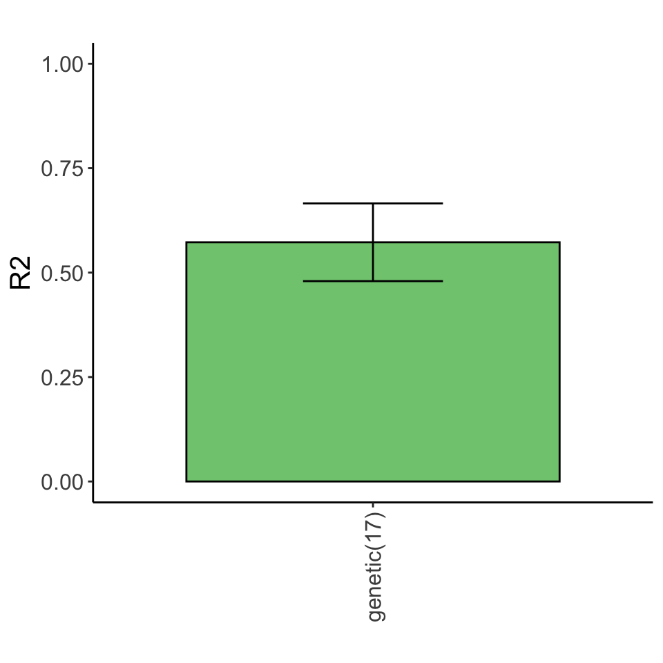
Lasso plot

heatMaps <- lassoPlot(lassoResults, cleanData, freqCut = 0.8,setNumber = 1, legend = FALSE, scaleFac = 1)
heatMaps

$Doxorubicin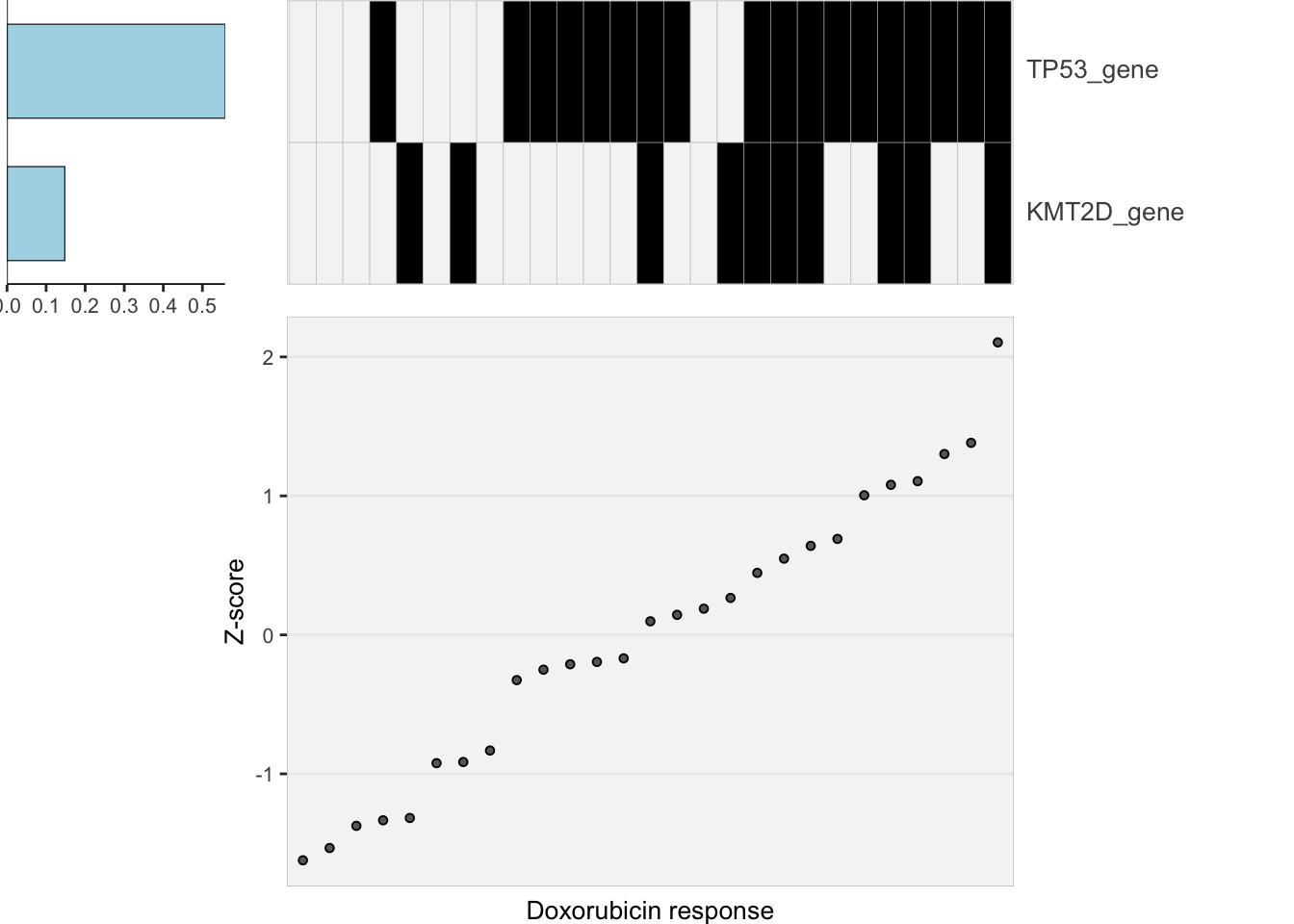

Only protein as predictors

Clean and integrate multi-omics data

inclSet<-list(Protein=protMat)
cleanData <- generateData(responseList, inclSet, censor = 5)

Run lasso

set.seed(2021)
lassoResults <- list()
for (eachMeasure in names(cleanData$allResponse)) {
  dataResult <- list()
  for (eachDataset in names(cleanData$allExplain[[eachMeasure]])) {
    y <- cleanData$allResponse[[eachMeasure]]
    X <- cleanData$allExplain[[eachMeasure]][[eachDataset]]
  
   
    glmRes <- runGlm(X, y, method = "lasso", repeats = 50, folds = 3)
    dataResult[[eachDataset]] <- glmRes 
  }
  lassoResults[[eachMeasure]] <- dataResult
  
}

Variance explained

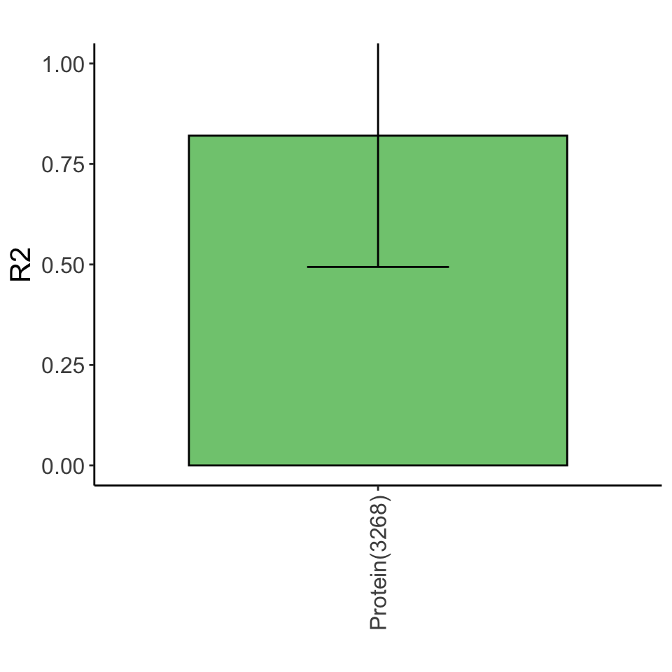
Lasso plot

heatMaps <- lassoPlot(lassoResults, cleanData, freqCut = 0.8,setNumber = 1, legend = FALSE, scaleFac = 1)
heatMaps

$Doxorubicin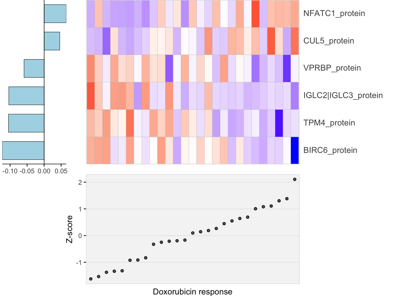

Only rna as predictors

Clean and integrate multi-omics data

inclSet<-list(RNA=exprMat)
cleanData <- generateData(responseList, inclSet, censor = 5)

Run lasso

set.seed(2021)
lassoResults <- list()
for (eachMeasure in names(cleanData$allResponse)) {
  dataResult <- list()
  for (eachDataset in names(cleanData$allExplain[[eachMeasure]])) {
    y <- cleanData$allResponse[[eachMeasure]]
    X <- cleanData$allExplain[[eachMeasure]][[eachDataset]]
  
   
    glmRes <- runGlm(X, y, method = "lasso", repeats = 50, folds = 3)
    dataResult[[eachDataset]] <- glmRes 
  }
  lassoResults[[eachMeasure]] <- dataResult
  
}

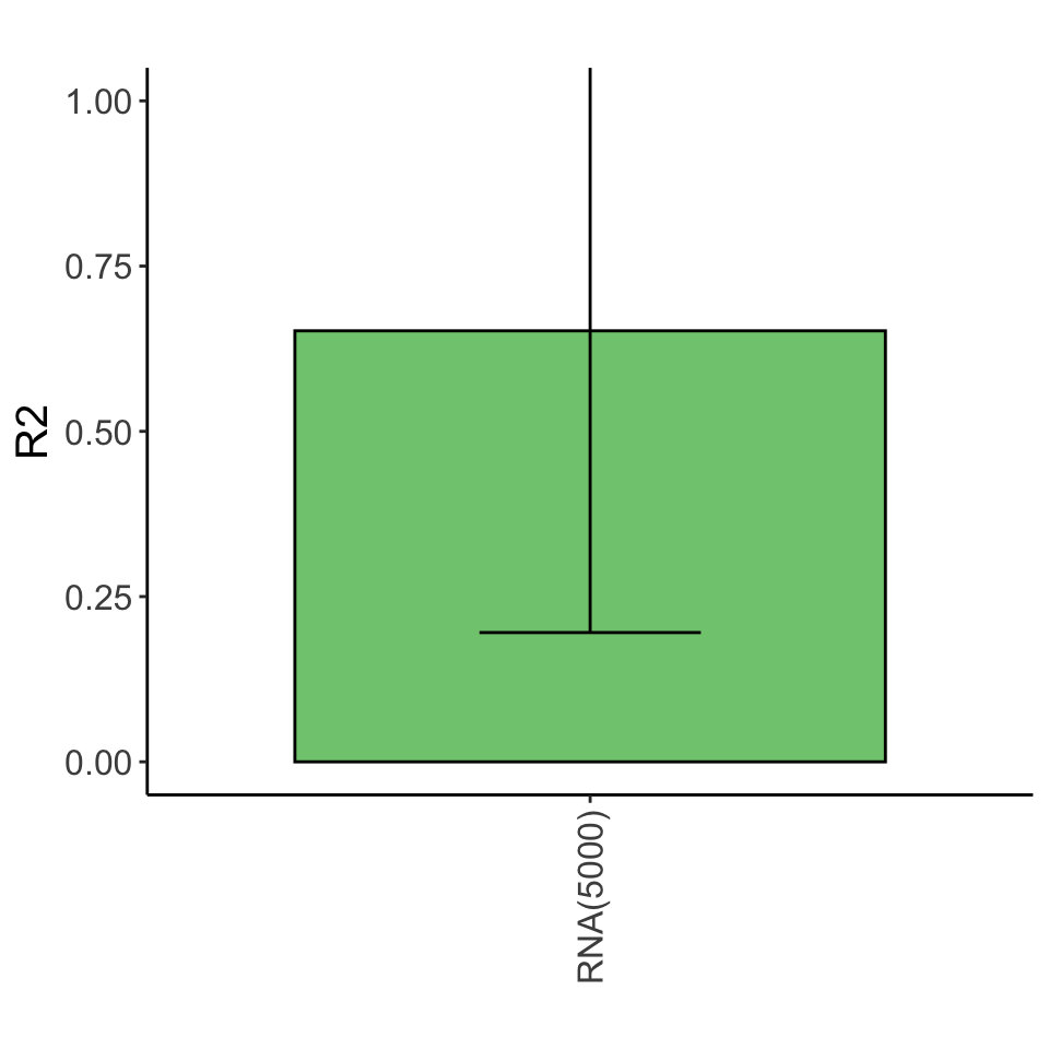
Variance explained

Only metabolites as predictors

Clean and integrate multi-omics data

inclSet<-list(Metabolite=metaMat)
cleanData <- generateData(responseList, inclSet, censor = 5)

Run lasso

set.seed(2021)
lassoResults <- list()
for (eachMeasure in names(cleanData$allResponse)) {
  dataResult <- list()
  for (eachDataset in names(cleanData$allExplain[[eachMeasure]])) {
    y <- cleanData$allResponse[[eachMeasure]]
    X <- cleanData$allExplain[[eachMeasure]][[eachDataset]]
  
   
    glmRes <- runGlm(X, y, method = "lasso", repeats = 50, folds = 3)
    dataResult[[eachDataset]] <- glmRes 
  }
  lassoResults[[eachMeasure]] <- dataResult
  
}

Variance explained

Lasso plot

heatMaps <- lassoPlot(lassoResults, cleanData, freqCut = 0.8,setNumber = 1, legend = FALSE, scaleFac = 1)
heatMaps

$Doxorubicin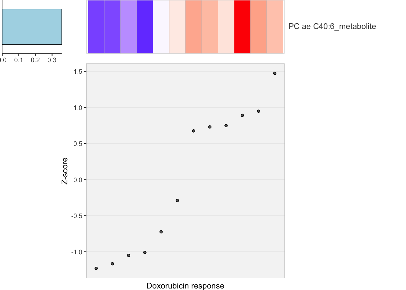

Heatmap of selected features

All combined

Clean and integrate multi-omics data

inclSet<-list(Gene=geneMat, Protein = protMat, RNA = exprMat, Metabolite = metaMat)
cleanData <- generateData(responseList, inclSet, censor = 5)

set.seed(2021)
lassoResults <- list()
for (eachMeasure in names(cleanData$allResponse)) {
  dataResult <- list()
  for (eachDataset in names(cleanData$allExplain[[eachMeasure]])) {
    y <- cleanData$allResponse[[eachMeasure]]
    X <- cleanData$allExplain[[eachMeasure]][[eachDataset]]
  
   
    glmRes <- runGlm(X, y, method = "lasso", repeats = 50, folds = 3)
    dataResult[[eachDataset]] <- glmRes 
  }
  lassoResults[[eachMeasure]] <- dataResult
  
}

varList <- plotVar(lassoResults)

cowplot::plot_grid(plotlist = varList, ncol=1)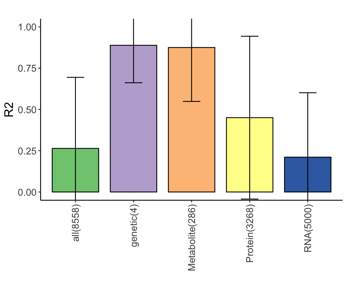

Combined

heatMaps <- lassoPlot(lassoResults, cleanData, freqCut = 0.2, setNumber = 5, legend = FALSE, scaleFac = 1)
plot_grid(heatMaps$Doxorubicin)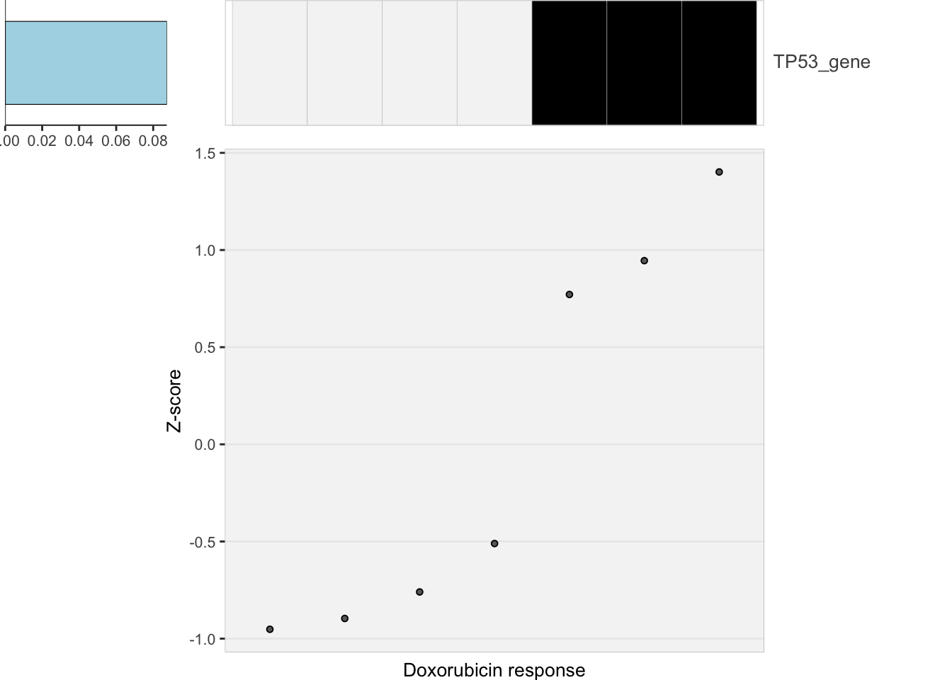

Sample size is perhaps too small for LASSO

sessionInfo()

R version 4.2.0 (2022-04-22)
Platform: x86_64-apple-darwin17.0 (64-bit)
Running under: macOS Big Sur/Monterey 10.16

Matrix products: default
BLAS:   /Library/Frameworks/R.framework/Versions/4.2/Resources/lib/libRblas.0.dylib
LAPACK: /Library/Frameworks/R.framework/Versions/4.2/Resources/lib/libRlapack.dylib

locale:
[1] en_US.UTF-8/en_US.UTF-8/en_US.UTF-8/C/en_US.UTF-8/en_US.UTF-8

attached base packages:
[1] stats4    stats     graphics  grDevices utils     datasets  methods  
[8] base     

other attached packages:
 [1] gtable_0.3.0                glmnet_4.1-4               
 [3] Matrix_1.4-1                pheatmap_1.0.12            
 [5] piano_2.12.0                forcats_0.5.1              
 [7] stringr_1.4.0               dplyr_1.0.9                
 [9] purrr_0.3.4                 readr_2.1.2                
[11] tidyr_1.2.0                 tibble_3.1.7               
[13] ggplot2_3.3.6               tidyverse_1.3.1            
[15] proDA_1.10.0                cowplot_1.1.1              
[17] DESeq2_1.36.0               SummarizedExperiment_1.26.1
[19] Biobase_2.56.0              GenomicRanges_1.48.0       
[21] GenomeInfoDb_1.32.2         IRanges_2.30.0             
[23] S4Vectors_0.34.0            BiocGenerics_0.42.0        
[25] MatrixGenerics_1.8.0        matrixStats_0.62.0         
[27] limma_3.52.2                jyluMisc_0.1.5             

loaded via a namespace (and not attached):
  [1] utf8_1.2.2                  shinydashboard_0.7.2       
  [3] reticulate_1.25             tidyselect_1.1.2           
  [5] RSQLite_2.2.14              AnnotationDbi_1.58.0       
  [7] htmlwidgets_1.5.4           grid_4.2.0                 
  [9] BiocParallel_1.30.3         Rtsne_0.16                 
 [11] maxstat_0.7-25              munsell_0.5.0              
 [13] preprocessCore_1.58.0       codetools_0.2-18           
 [15] DT_0.23                     withr_2.5.0                
 [17] colorspace_2.0-3            filelock_1.0.2             
 [19] highr_0.9                   knitr_1.39                 
 [21] rstudioapi_0.13             ggsignif_0.6.3             
 [23] labeling_0.4.2              git2r_0.30.1               
 [25] slam_0.1-50                 GenomeInfoDbData_1.2.8     
 [27] KMsurv_0.1-5                bit64_4.0.5                
 [29] farver_2.1.0                rhdf5_2.40.0               
 [31] rprojroot_2.0.3             basilisk_1.8.0             
 [33] vctrs_0.4.1                 generics_0.1.2             
 [35] TH.data_1.1-1               xfun_0.31                  
 [37] sets_1.0-21                 R6_2.5.1                   
 [39] locfit_1.5-9.5              rhdf5filters_1.8.0         
 [41] bitops_1.0-7                cachem_1.0.6               
 [43] fgsea_1.22.0                DelayedArray_0.22.0        
 [45] assertthat_0.2.1            promises_1.2.0.1           
 [47] scales_1.2.0                multcomp_1.4-19            
 [49] extraDistr_1.9.1            egg_0.4.5                  
 [51] affy_1.74.0                 sandwich_3.0-2             
 [53] workflowr_1.7.0             rlang_1.0.2                
 [55] genefilter_1.78.0           splines_4.2.0              
 [57] rstatix_0.7.0               broom_0.8.0                
 [59] reshape2_1.4.4              BiocManager_1.30.18        
 [61] yaml_2.3.5                  abind_1.4-5                
 [63] modelr_0.1.8                crosstalk_1.2.0            
 [65] backports_1.4.1             httpuv_1.6.5               
 [67] tools_4.2.0                 relations_0.6-12           
 [69] affyio_1.66.0               ellipsis_0.3.2             
 [71] gplots_3.1.3                jquerylib_0.1.4            
 [73] RColorBrewer_1.1-3          MultiAssayExperiment_1.22.0
 [75] plyr_1.8.7                  Rcpp_1.0.8.3               
 [77] visNetwork_2.1.0            zlibbioc_1.42.0            
 [79] RCurl_1.98-1.7              basilisk.utils_1.8.0       
 [81] ggpubr_0.4.0                zoo_1.8-10                 
 [83] haven_2.5.0                 ggrepel_0.9.1              
 [85] cluster_2.1.3               exactRankTests_0.8-35      
 [87] fs_1.5.2                    magrittr_2.0.3             
 [89] data.table_1.14.2           reprex_2.0.1               
 [91] survminer_0.4.9             mvtnorm_1.1-3              
 [93] hms_1.1.1                   shinyjs_2.1.0              
 [95] mime_0.12                   evaluate_0.15              
 [97] xtable_1.8-4                XML_3.99-0.10              
 [99] readxl_1.4.0                shape_1.4.6                
[101] gridExtra_2.3               compiler_4.2.0             
[103] KernSmooth_2.23-20          crayon_1.5.1               
[105] htmltools_0.5.2             mgcv_1.8-40                
[107] later_1.3.0                 tzdb_0.3.0                 
[109] geneplotter_1.74.0          lubridate_1.8.0            
[111] DBI_1.1.3                   corrplot_0.92              
[113] dbplyr_2.2.0                MASS_7.3-57                
[115] car_3.1-0                   cli_3.3.0                  
[117] vsn_3.64.0                  marray_1.74.0              
[119] parallel_4.2.0              igraph_1.3.2               
[121] pkgconfig_2.0.3             km.ci_0.5-6                
[123] dir.expiry_1.4.0            foreach_1.5.2              
[125] xml2_1.3.3                  annotate_1.74.0            
[127] bslib_0.3.1                 XVector_0.36.0             
[129] drc_3.0-1                   rvest_1.0.2                
[131] digest_0.6.29               Biostrings_2.64.0          
[133] rmarkdown_2.14              cellranger_1.1.0           
[135] fastmatch_1.1-3             survMisc_0.5.6             
[137] uwot_0.1.11                 shiny_1.7.1                
[139] gtools_3.9.2.2              lifecycle_1.0.1            
[141] nlme_3.1-158                jsonlite_1.8.0             
[143] Rhdf5lib_1.18.2             carData_3.0-5              
[145] fansi_1.0.3                 pillar_1.7.0               
[147] lattice_0.20-45             KEGGREST_1.36.2            
[149] fastmap_1.1.0               httr_1.4.3                 
[151] plotrix_3.8-2               survival_3.3-1             
[153] glue_1.6.2                  iterators_1.0.14           
[155] png_0.1-7                   bit_4.0.4                  
[157] HDF5Array_1.24.1            stringi_1.7.6              
[159] sass_0.4.1                  blob_1.2.3                 
[161] caTools_1.18.2              memoise_2.0.1

Compare the signature of Doxorubicin resistant and sensitive DLBCL cell lines (using continous response variable)

Junyan Lu

2022-06-10

Load libraries and datasets

Data preprocessing

Drug screen data (the cell line screen data from Tobias)

Genomics

Processing genomics data

T-test

Association with proteomics

Preprocessing proteomic data

Identify proteins differentially expressed

Enrichment analysis

Metabolimics

Process metabolomic data

Differential metabolites abundance

Differential gene expression analysis based on public data

Proprocessing

Differential expression using limma

Enrichment analysis

MOFA analysis

Preprocessing

Create MOFA object

Define MOFA options

Data options

Model options

Training options

Train the MOFA model

Preliminary analysis of the results

Factor heatmap

Correlation between factors and annotations

Focus on F1 (Doxorubicine response)

Focus on F3 (Subtype)

LASSO regression for predicting Doxorubicine responses

Preprocessing data

Feature selection with LASSO penalty

Only genetics as predictors

Only protein as predictors

Only rna as predictors

Only metabolites as predictors

Heatmap of selected features

All combined