Integrative analysis using MOFA
Junyan Lu
2022-05-04
Last updated: 2022-09-21
Checks: 5 1
Knit directory: combiDLBCL/analysis/
This reproducible R Markdown analysis was created with workflowr (version 1.7.0). The Checks tab describes the reproducibility checks that were applied when the results were created. The Past versions tab lists the development history.
Great job! The global environment was empty. Objects defined in the global environment can affect the analysis in your R Markdown file in unknown ways. For reproduciblity it’s best to always run the code in an empty environment.
The command set.seed(20220425) was run prior to running
the code in the R Markdown file. Setting a seed ensures that any results
that rely on randomness, e.g. subsampling or permutations, are
reproducible.
Great job! Recording the operating system, R version, and package versions is critical for reproducibility.
Nice! There were no cached chunks for this analysis, so you can be confident that you successfully produced the results during this run.
Great job! Using relative paths to the files within your workflowr project makes it easier to run your code on other machines.
Tracking code development and connecting the code version to the
results is critical for reproducibility. To start using Git, open the
Terminal and type git init in your project directory.
This project is not being versioned with Git. To obtain the full
reproducibility benefits of using workflowr, please see
?wflow_start.
Load libraries
Data preprocessing
Select DLBCL cell line only
load("../data/Screen.CL19.RData")
cellList <- unique(filter(Screen.CL19, str_detect(Entity, "DLBCL"))$Name)
Drug screen data
Subset for Pola plates
#load pre-processed data
load("../output/screenData.RData")
screenData <- filter(screenData, Plate =="CHP:Pola", Drug_A != "AZD7762") %>%
  mutate(Name = ifelse(Name %in% "Karpas1106p","Karpas-1106p",Name))
Get combi-drug
singleViab <- filter(screenData, Drug_B.Conc ==0, Drug_A.Conc!=0) %>%
  mutate(Drug = Drug_A, Conc = Drug_A.Conc, ConcStep = Drug_A.ConcStep) %>%
  select(Name, Drug, Conc, ConcStep, normVal)
Get base-drug
baseViab <- filter(screenData, Drug_A.Conc ==0, Drug_B.Conc!=0) %>%
  mutate(Drug = Drug_B, Conc = Drug_B.Conc, ConcStep = Drug_B.ConcStep) %>%
  select(Name, Drug, Conc, ConcStep, normVal)
Combine and summarise
viabTab.conc <- bind_rows(singleViab, baseViab) #individual concentration
viabTab <- group_by(viabTab.conc, Name, Drug) %>%
  summarise(viab = calcAUC(normVal, Conc)) %>%
  ungroup()

drugMat <- viabTab %>% pivot_wider(names_from = Name, values_from = viab) %>%
  column_to_rownames("Drug") %>% as.matrix()

dim(drugMat)
[1] 28 32Drug combination index
Get combination effect
screenSub <- filter(screenData, Drug_B == "CHP_Pola")

comTab <- filter(screenSub, Drug_A.Conc >0, Drug_B.Conc >0) %>%
  select(Name, Drug_A, Drug_A.Conc, Drug_B, Drug_B.Conc, normVal) %>%
  dplyr::rename(viabObs = normVal)
drugATab <- filter(screenSub, Drug_A != "DMSO", Drug_B.Conc ==0) %>%
  select(Name, Drug_A, Drug_A.Conc, normVal, Drug_A.ConcStep) %>%
  dplyr::rename(viabA = normVal)
drugBTab <- filter(screenSub, Drug_A == "DMSO", Drug_B.Conc !=0) %>%
  select(Name, Drug_B, Drug_B.Conc, normVal) %>%
  dplyr::rename(viabB = normVal)
synTab <- comTab %>% left_join(drugATab, by =c("Name","Drug_A","Drug_A.Conc")) %>%
left_join(drugBTab, by = c("Name","Drug_B","Drug_B.Conc")) %>%
mutate(viabExp = viabA*viabB) %>%
mutate(CI = viabObs-viabExp,
logCI = log10(viabObs/viabExp)) %>%
group_by(Drug_A,Name) %>% summarise(meanCI = mean(CI))
combiMat <- pivot_wider(synTab, names_from = Name, values_from = meanCI) %>%
column_to_rownames("Drug_A") %>% as.matrix()
dim(combiMat)[1] 25 32Proteomics
library(SummarizedExperiment)
protData <- readRDS("../data/SC005_SummarizedExperiment_proteomics.RDS")
protData <- protData[, protData$condition %in% "U"]
protMat <- assay(protData)
protMatNorm <- PhosR::medianScaling(protMat, scale = FALSE)
protNorm <- protData
assay(protNorm) <- protMatNorm

protTab <- assay(protNorm) %>% as_tibble(rownames = "uniprotID") %>%
  pivot_longer(-uniprotID) %>%
  mutate(cellLine = colData(protNorm)[name,]$cell.line) %>%
  group_by(uniprotID, cellLine) %>%
  summarise(count = mean(value, na.rm=TRUE)) %>%
  ungroup() %>%
  mutate(symbol = rowData(protNorm)[uniprotID,]$Gene_name) %>%
  filter(!symbol %in% c("",NA)) %>% mutate(Name = cellLine)

protSub <- jyluMisc::tidyToSum(protTab, rowID = "uniprotID",colID = "cellLine",
                     values = "count", annoRow = "symbol", annoCol = "Name")

protMat <- assay(protSub)
rownames(protMat) <- rowData(protSub)$symbol
protMat <- protMat[!duplicated(rownames(protMat)),]
dim(protMat)
[1] 2640 13Metabolimics
metaData <- readRDS("../data/SC005_SummarizedExperiment_metabolomics.RDS")
metaData <- metaData[, metaData$condition %in% "U"]
metaMat <- assay(metaData)

metaMatNorm <- PhosR::medianScaling(metaMat, scale = FALSE)
metaNorm <- metaData
assay(metaNorm) <- metaMatNorm

metaTab <- assay(metaNorm) %>% as_tibble(rownames = "id") %>%
  pivot_longer(-id) %>%
  mutate(cellLine = colData(metaNorm)[name,]$cell.line) %>%
  group_by(id, cellLine) %>%
  summarise(count = mean(value, na.rm=TRUE)) %>%
  mutate(symbol = rowData(metaNorm)[id,]$metabolite,
         class = rowData(metaNorm)[id,]$class,
         Name = cellLine) %>%
  filter(!symbol %in% c("",NA))

metaSub <- jyluMisc::tidyToSum(metaTab, rowID = "id",colID = "cellLine",
                     values = "count", annoRow = c("symbol","class"), annoCol = "Name")

metaMat <- assay(metaSub)

dim(metaMat)
[1] 286 12Genomic data
Preprocessing genomics table
load("../data/SVs_filtered.RData")Summarise mutations:
count as gene mutation if there is at least one mutation within gene
#cellList <- intersect(intersect(colnames(drugMat), colnames(protMat)),colnames(metaMat))

mutTab <- filter(svTab, Name %in% colnames(drugMat)) %>%
  group_by(Name, Gene) %>% summarise(n = length(Name)) %>%
  arrange(desc(n))

#Get mutations occured at least in three cell lines
geneCount <- group_by(mutTab, Gene) %>% summarise(n=length(Name)) %>%
  filter(n>=5) %>% arrange(desc(n))
Only use mutations that occurred at least five time in all the cell lines
mutTabSub <- mutTab %>%
  mutate(status =1) %>% select(Name, Gene, status) %>%
  pivot_wider(names_from = "Gene", values_from = "status") %>%
  mutate_all(replace_na,0) %>%
  pivot_longer(-Name, names_to = "Gene", values_to = "status")%>%
  mutate(status = ifelse(Name %in% c("Pfeiffer", "OCI-LY-8") &
                           Gene == "TP53", 1,status)) %>% #fix TP53 mutation status of two cell lines
  filter(Gene %in% geneCount$Gene)

geneMat <- mutTabSub %>% pivot_wider(names_from = "Name", values_from = "status") %>%
  column_to_rownames("Gene") %>% as.matrix()

dim(geneMat)
[1] 10 32Create MOFA object
mofaData <- list(Drug = drugMat,
                 DrugCombo = combiMat,
                 Protein = protMat,
                 Mutation = geneMat,
                 Metabolite = metaMat)

# Create MultiAssayExperiment object
mofaData <- MultiAssayExperiment::MultiAssayExperiment(
  experiments = mofaData
)
Only keep samples that have at least four assays
useSamples <- MultiAssayExperiment::sampleMap(mofaData) %>%
  as_tibble() %>% group_by(primary) %>% summarise(n= length(assay)) %>%
  filter(n >= 4) %>% pull(primary)
mofaData <- mofaData[,useSamples]
MOFAobject <- create_mofa_from_MultiAssayExperiment(mofaData)Plot data overview
plot_data_overview(MOFAobject)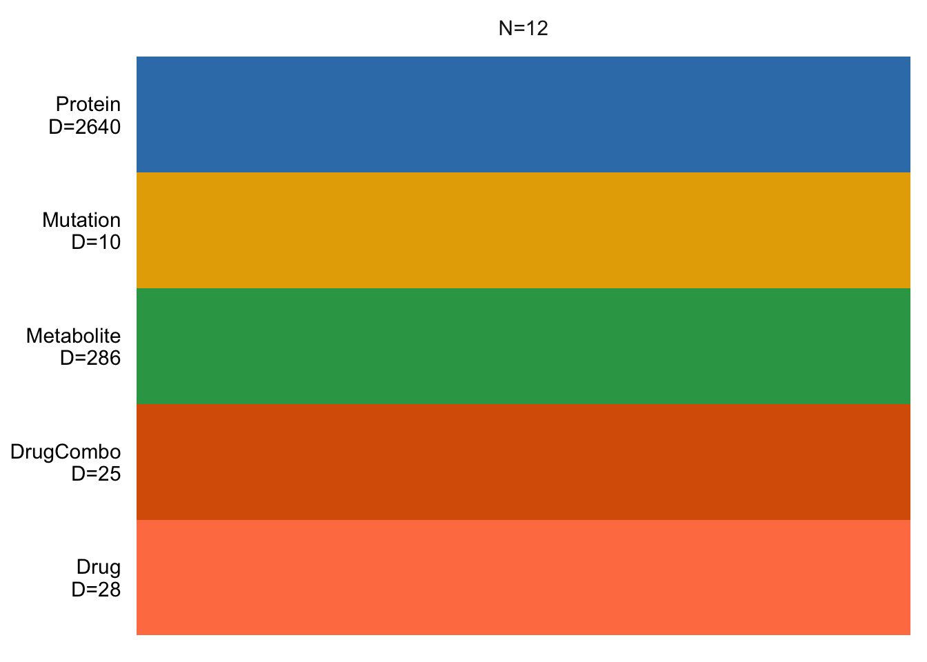
Define MOFA options
Data options
data_opts <- get_default_data_options(MOFAobject)
data_opts
$scale_views
[1] FALSE
$scale_groups
[1] FALSE
$center_groups
[1] TRUE
$use_float32
[1] FALSE
$views
[1] "Drug" "DrugCombo" "Protein" "Mutation" "Metabolite"
$groups
[1] "group1"Model options
model_opts <- get_default_model_options(MOFAobject)
model_opts$num_factors <- 10
model_opts
$likelihoods
Drug DrugCombo Protein Mutation Metabolite
"gaussian" "gaussian" "gaussian" "gaussian" "gaussian"
$num_factors
[1] 10
$spikeslab_factors
[1] FALSE
$spikeslab_weights
[1] TRUE
$ard_factors
[1] FALSE
$ard_weights
[1] TRUEChange the likely hood of Mutations to “bernoulli
model_opts$likelihoods[["Mutation"]] <- "bernoulli"
model_opts$likelihoods
Drug DrugCombo Protein Mutation Metabolite
"gaussian" "gaussian" "gaussian" "bernoulli" "gaussian" Training options
train_opts <- get_default_training_options(MOFAobject)
train_opts$convergence_mode <- "slow"
train_opts$seed <- 2022
train_opts$maxiter <- 10000
train_opts
$maxiter
[1] 10000
$convergence_mode
[1] "slow"
$drop_factor_threshold
[1] -1
$verbose
[1] FALSE
$startELBO
[1] 1
$freqELBO
[1] 5
$stochastic
[1] FALSE
$gpu_mode
[1] FALSE
$seed
[1] 2022
$outfile
NULL
$weight_views
[1] FALSE
$save_interrupted
[1] FALSEChange drop threshold to 0.01
train_opts$drop_factor_threshold <-0.01Train the MOFA model
Prepare MOFA object
MOFAobject <- prepare_mofa(MOFAobject,
  data_options = data_opts,
  model_options = model_opts,
  training_options = train_opts
)
Training
MOFAobject <- run_mofa(MOFAobject)
saveRDS(MOFAobject,"../output/mofaDLBCL.rds")
Preliminary analysis of the results
MOFAobject <- readRDS("../output/mofaDLBCL.rds")Factor correlation matrix
plot_factor_cor(MOFAobject)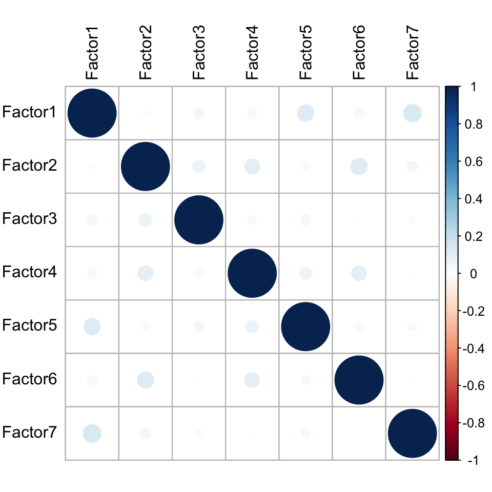
Variance explained
plot_variance_explained(MOFAobject, max_r2=15)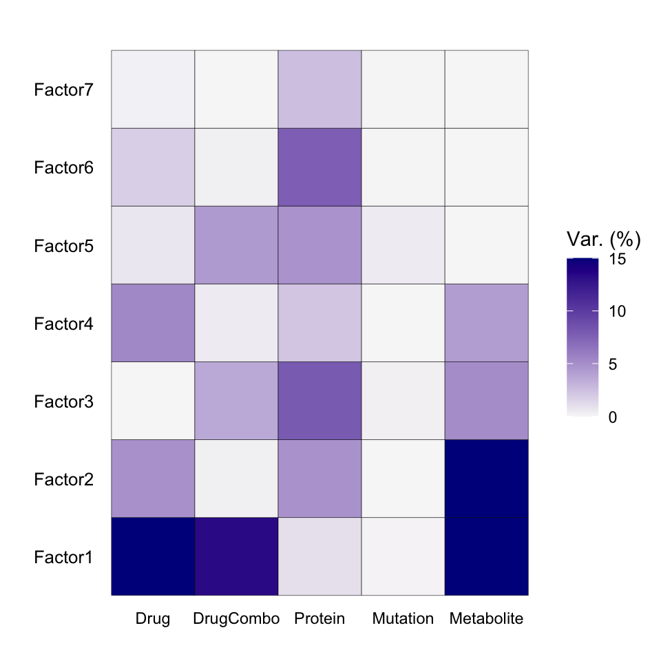
Total variance explained
plot_variance_explained(MOFAobject, plot_total = T)[[2]]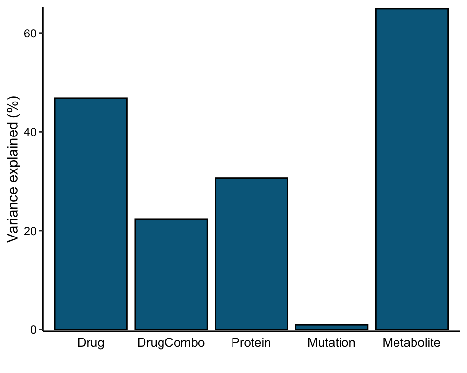
Factor heatmap
library(pheatmap)
#gene annotation
facMat <- t(get_factors(MOFAobject)[[1]])

seleGenes <- c("TP53","EP300","BCL2","KMT2D")

colAnno <- tibble(Name = colnames(facMat)) %>%
  left_join(mutTabSub,by="Name") %>% filter(Gene %in% seleGenes) %>%
  pivot_wider(names_from = "Gene", values_from = "status") %>%
  data.frame() %>% column_to_rownames("Name")


pheatmap(facMat, clustering_method = "complete", annotation_col = colAnno)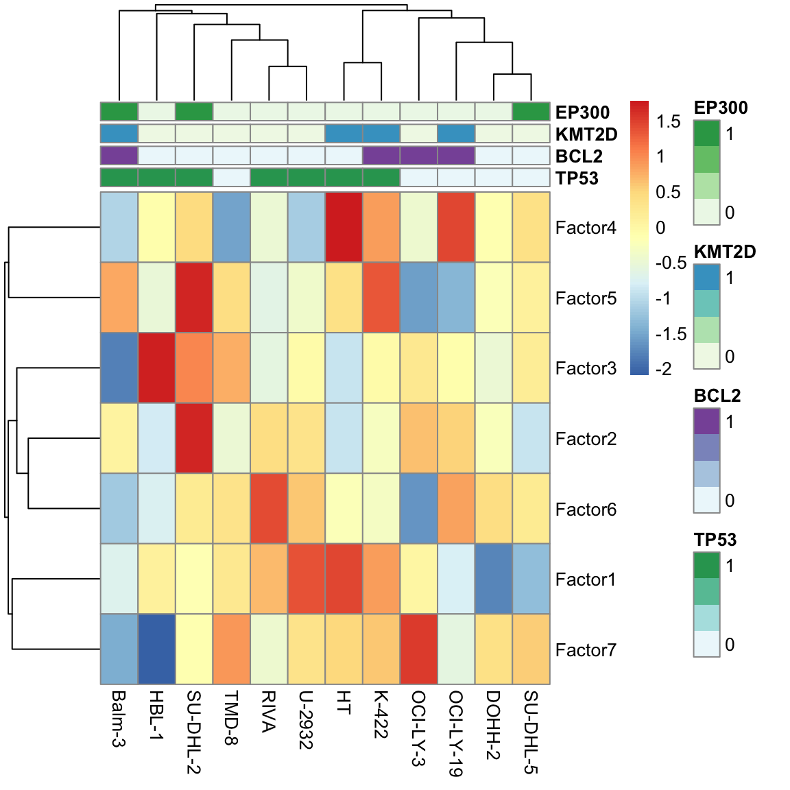
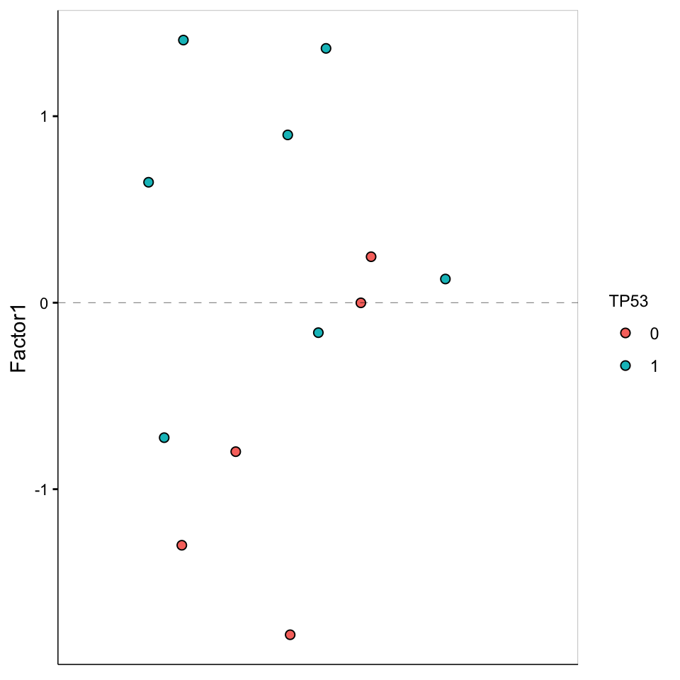
Focus on F1
Factor values
plot_factor(MOFAobject,
  factors = 1,
  color_by = "TP53"
)
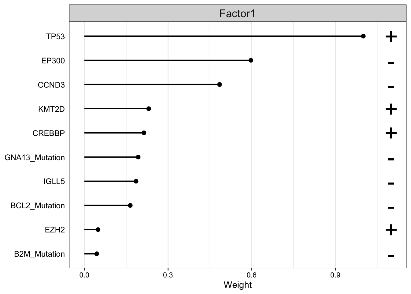
Weight of genomic features
plot_top_weights(MOFAobject,
 view = "Mutation",
 factor = 1,
 nfeatures = 10,     # Top number of features to highlight
 scale = T           # Scale weights from -1 to 1
)
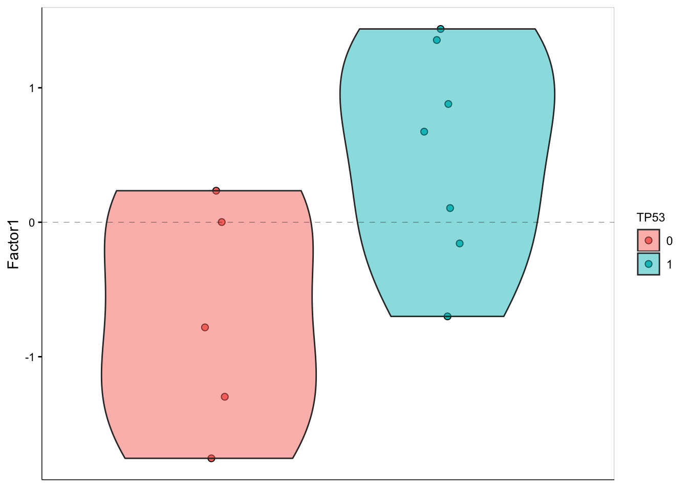
F1 values versus TP53 mutation
plot_factor(MOFAobject,
  factors = 1,
  color_by = "TP53",
  add_violin = TRUE,
  dodge = TRUE
)
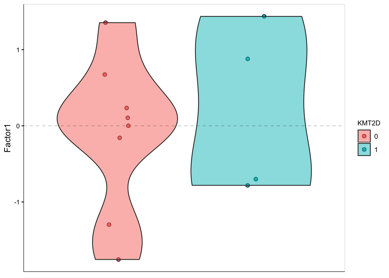
F1 values versus KMT2D mutation
plot_factor(MOFAobject,
  factors = 1,
  color_by = "KMT2D",
  add_violin = TRUE,
  dodge = TRUE
)
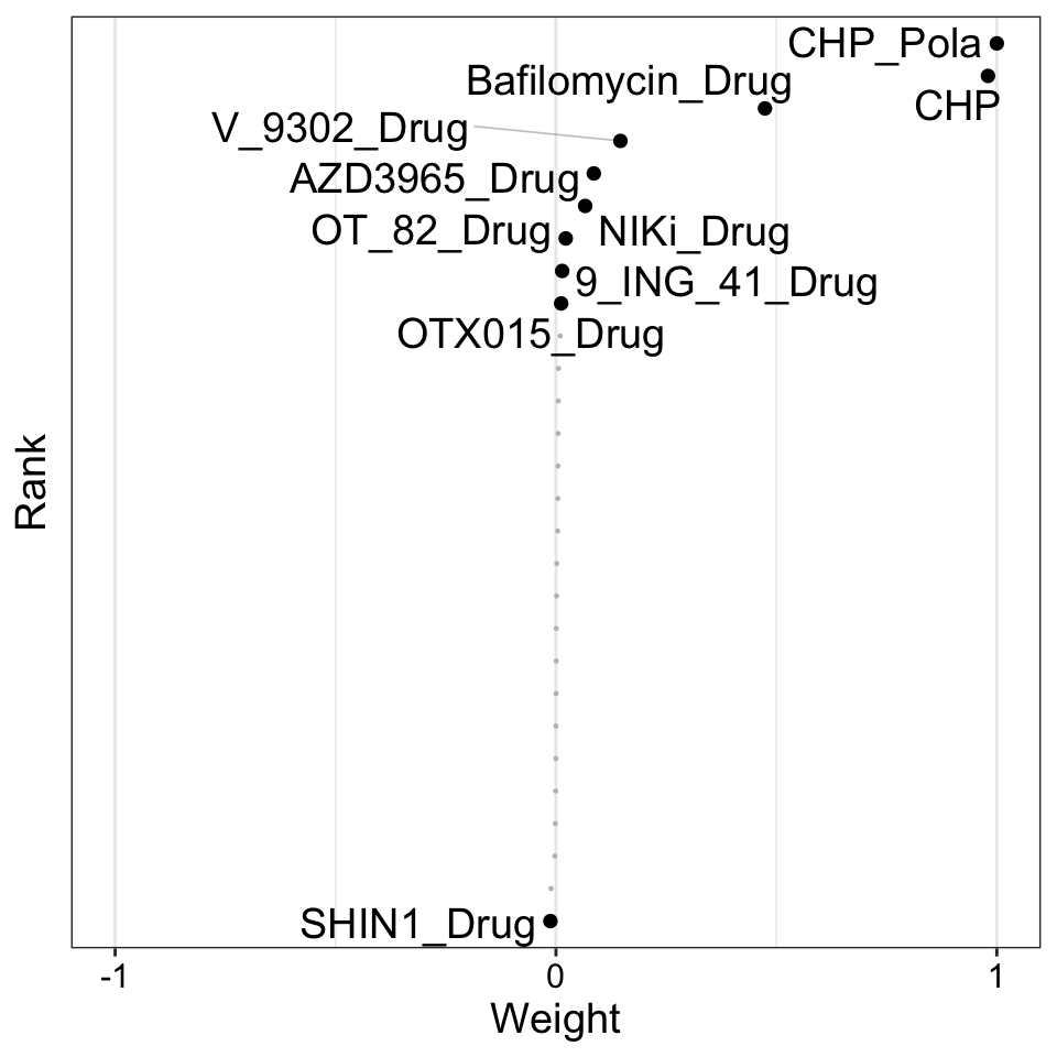
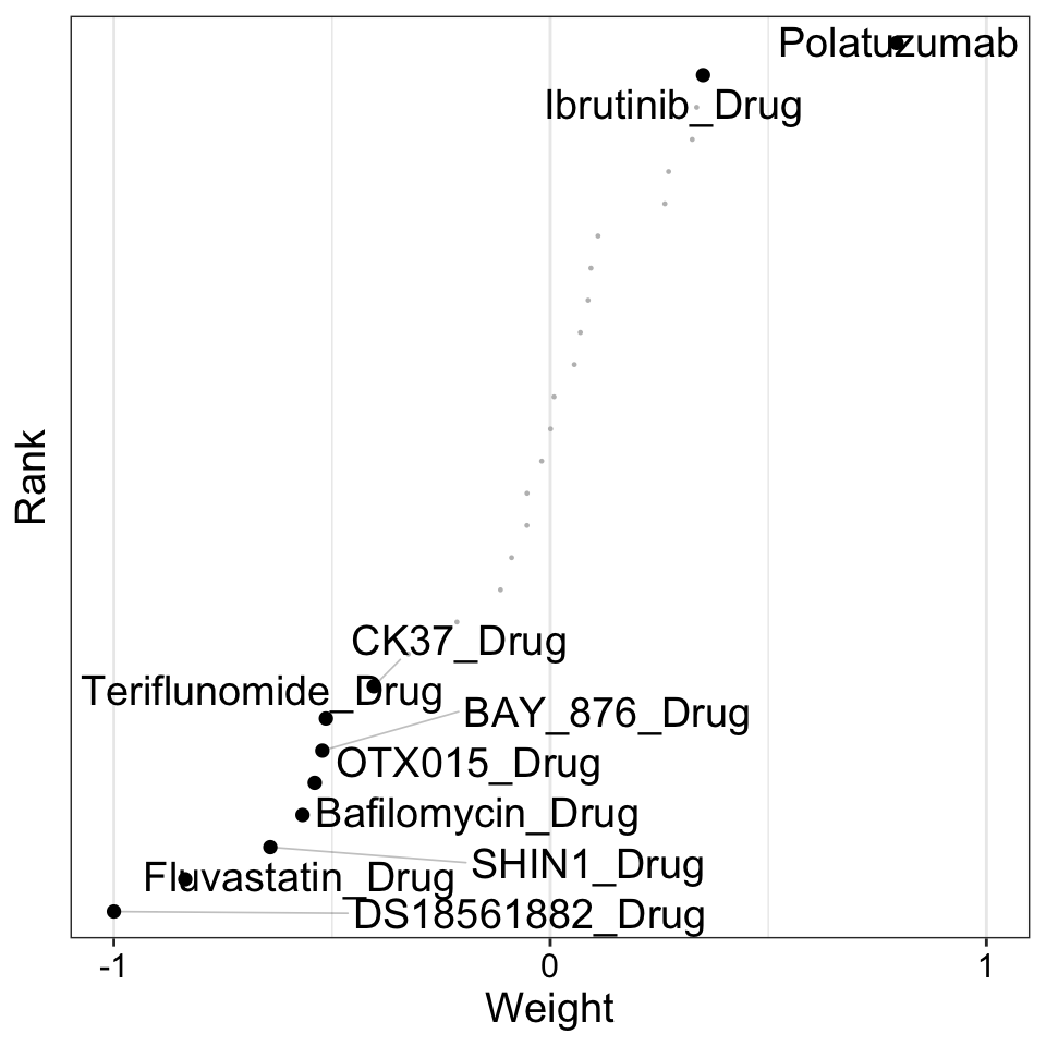
Weight of drug features
plot_weights(MOFAobject,
 view = "Drug",
 factor = 1,
 nfeatures = 10,     # Top number of features to highlight
 scale = T           # Scale weights from -1 to 1
)
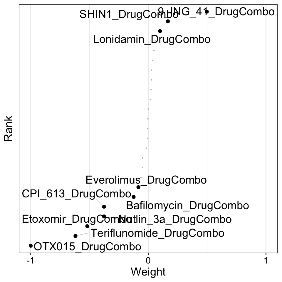
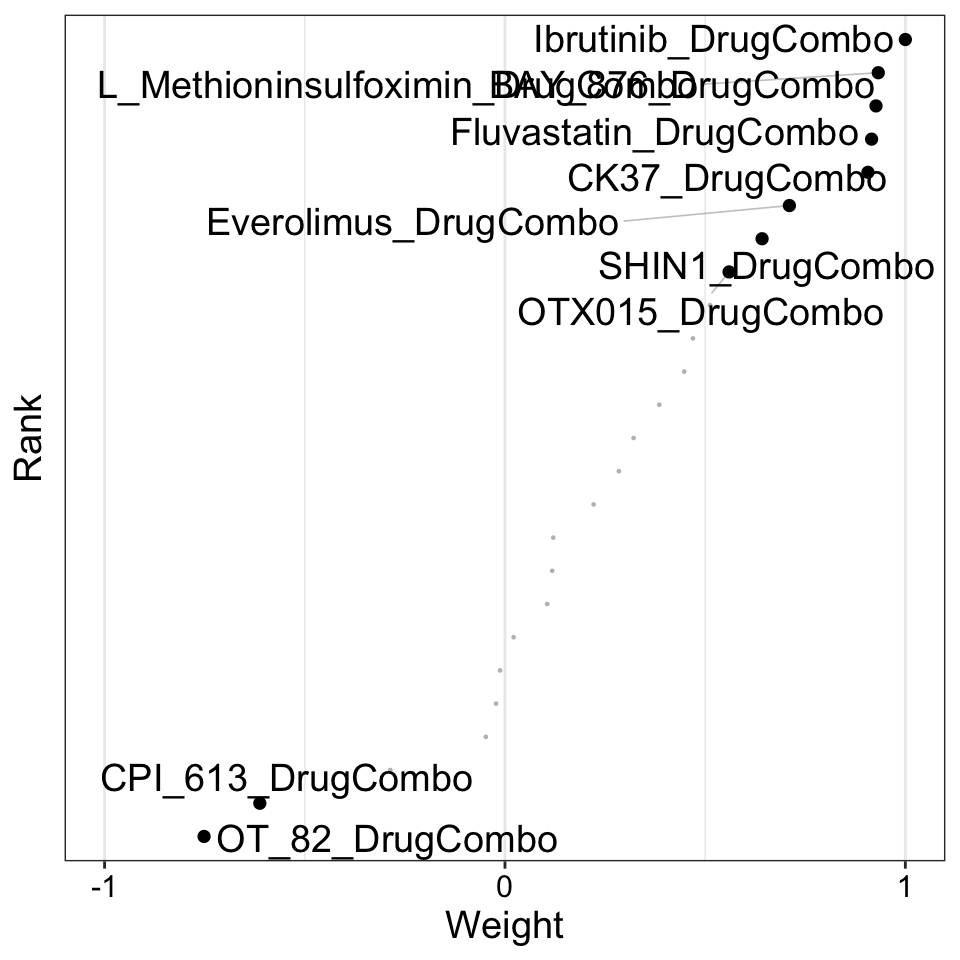
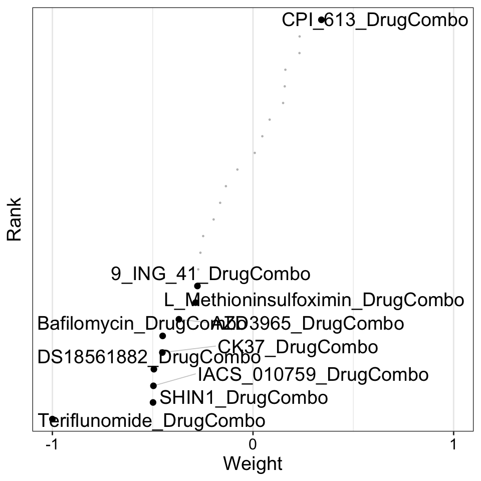
Weight of drug combination index features
plot_weights(MOFAobject,
 view = "DrugCombo",
 factor = 1,
 nfeatures = 10,     # Top number of features to highlight
 scale = T           # Scale weights from -1 to 1
)
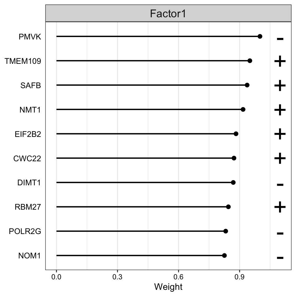
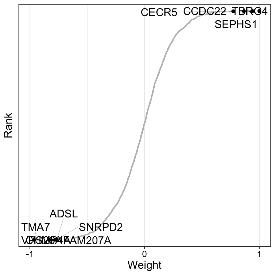
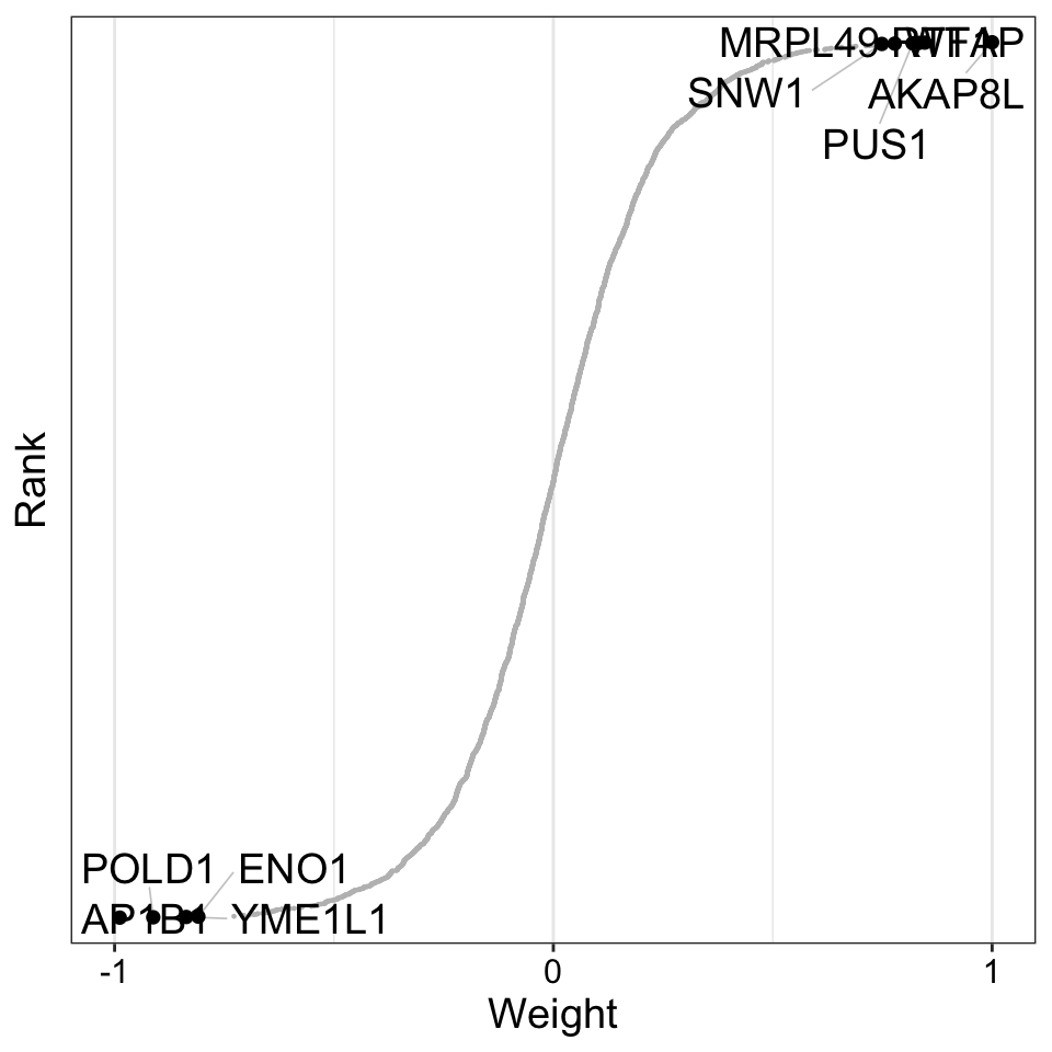
Weight of protein features
plot_top_weights(MOFAobject,
 view = "Protein",
 factor = 1,
 nfeatures = 10,     # Top number of features to highlight
 scale = T           # Scale weights from -1 to 1
)
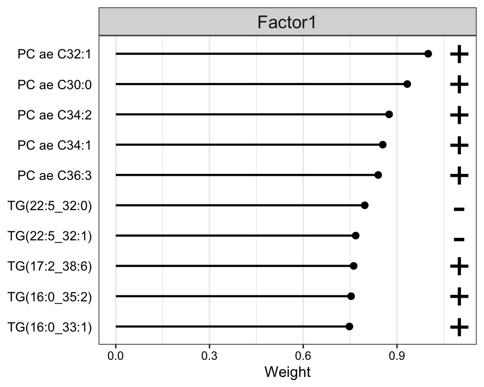
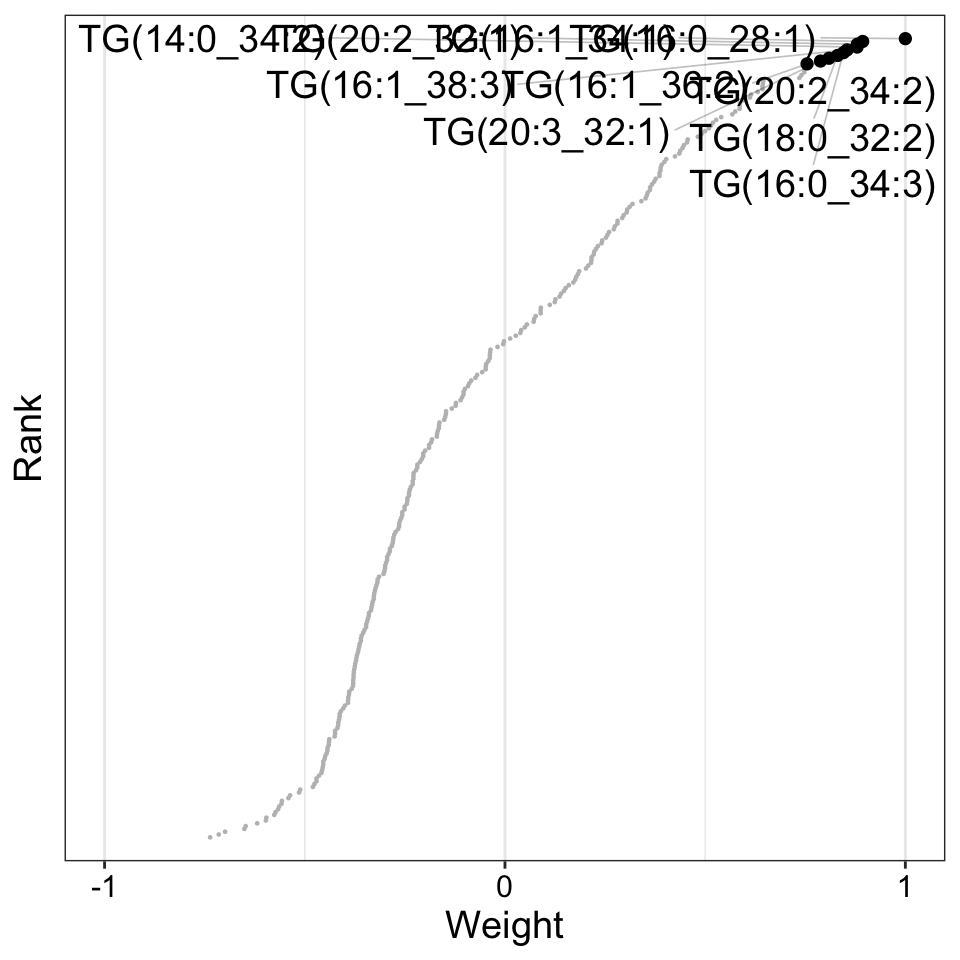
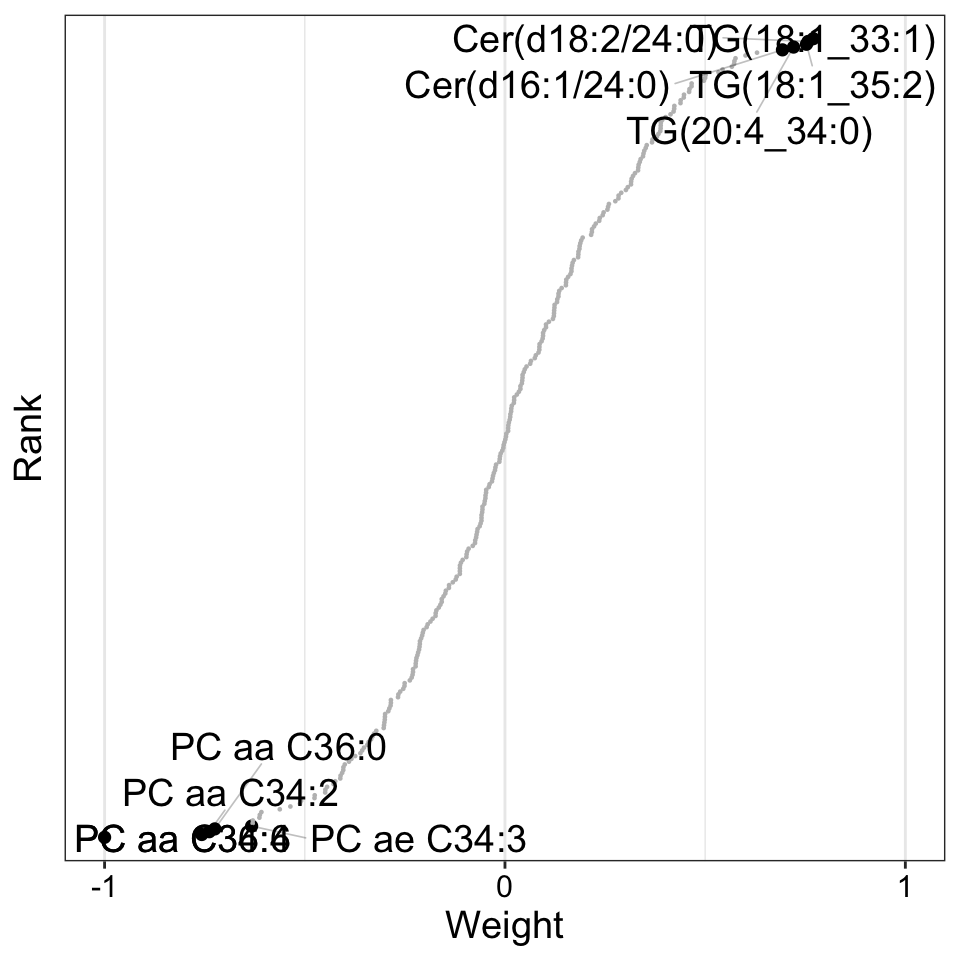
Weight of metabolites features
plot_top_weights(MOFAobject,
 view = "Metabolite",
 factor = 1,
 nfeatures = 10,     # Top number of features to highlight
 scale = T           # Scale weights from -1 to 1
)
Focus on F2
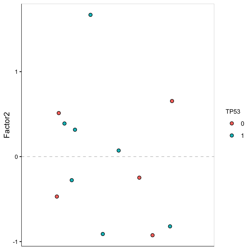
Factor 2 values
plot_factor(MOFAobject,
  factors = 2,
  color_by = "TP53"
)
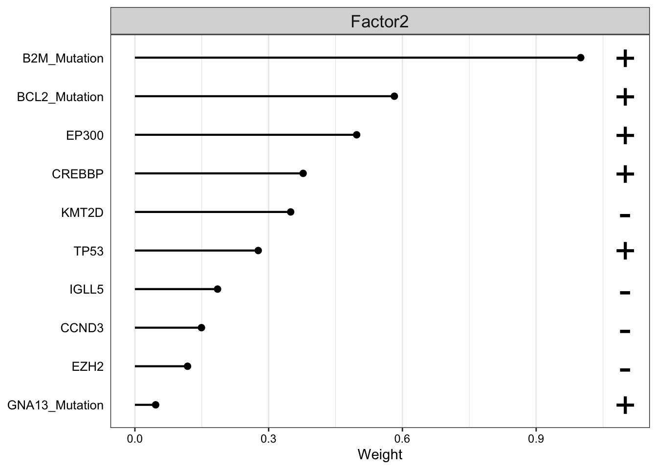
Weight of genomic features
plot_top_weights(MOFAobject,
 view = "Mutation",
 factor =2,
 nfeatures = 10,     # Top number of features to highlight
 scale = T           # Scale weights from -1 to 1
)
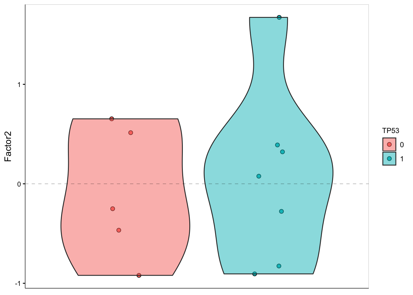
LF2 values versus TTN mutation
plot_factor(MOFAobject,
  factors = 2,
  color_by = "TP53",
  add_violin = TRUE,
  dodge = TRUE
)
Weight of drug features
plot_weights(MOFAobject,
 view = "Drug",
 factor = 2,
 nfeatures = 10,     # Top number of features to highlight
 scale = T           # Scale weights from -1 to 1
)
Weight of drug combo features
plot_weights(MOFAobject,
 view = "DrugCombo",
 factor = 2,
 nfeatures = 10,     # Top number of features to highlight
 scale = T           # Scale weights from -1 to 1
)
Weight of protein features
plot_weights(MOFAobject,
 view = "Protein",
 factor = 2,
 nfeatures = 10,     # Top number of features to highlight
 scale = T           # Scale weights from -1 to 1
)
Weight of metabolites features
plot_weights(MOFAobject,
 view = "Metabolite",
 factor = 2,
 nfeatures = 10,     # Top number of features to highlight
 scale = T           # Scale weights from -1 to 1
)
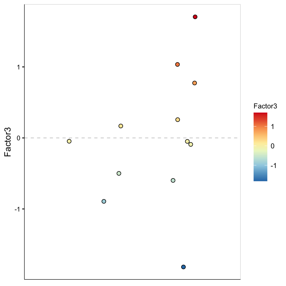
Focus on F3
Factor 3 values
plot_factor(MOFAobject,
  factors = 3,
  color_by = "Factor3"
)
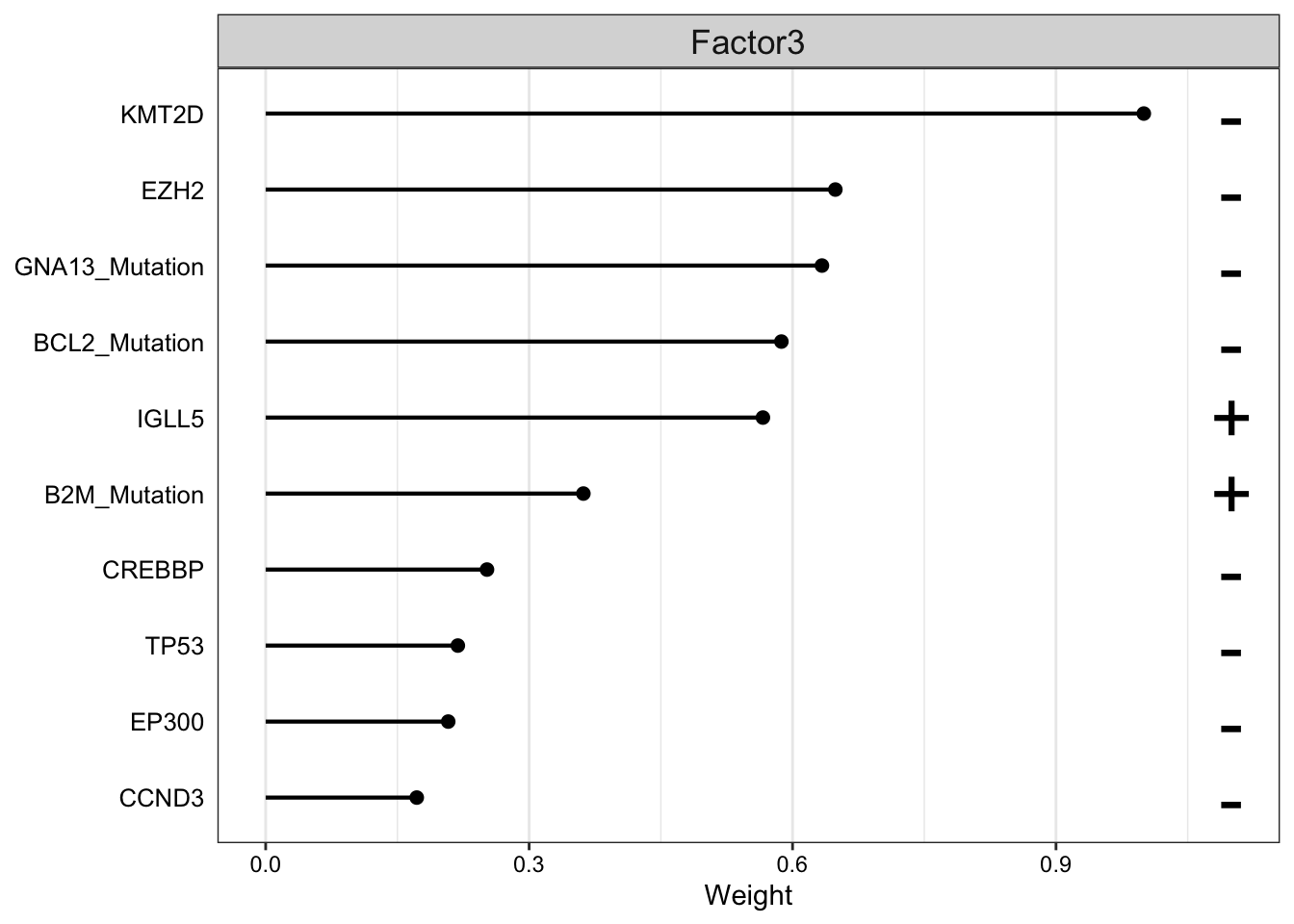
Weight of genomic features on LF3
plot_top_weights(MOFAobject,
 view = "Mutation",
 factor =3,
 nfeatures = 10,     # Top number of features to highlight
 scale = T           # Scale weights from -1 to 1
)
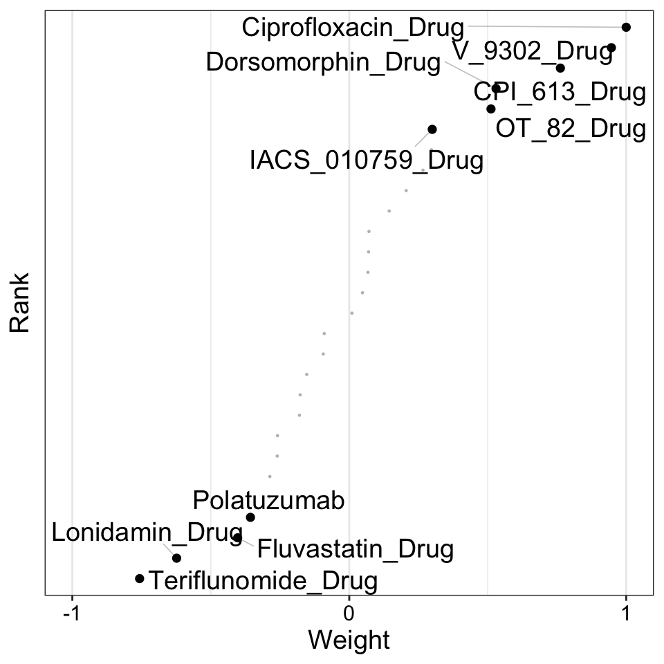
Weight of drug features on LF3
plot_weights(MOFAobject,
 view = "Drug",
 factor = 3,
 nfeatures = 10,     # Top number of features to highlight
 scale = T           # Scale weights from -1 to 1
)
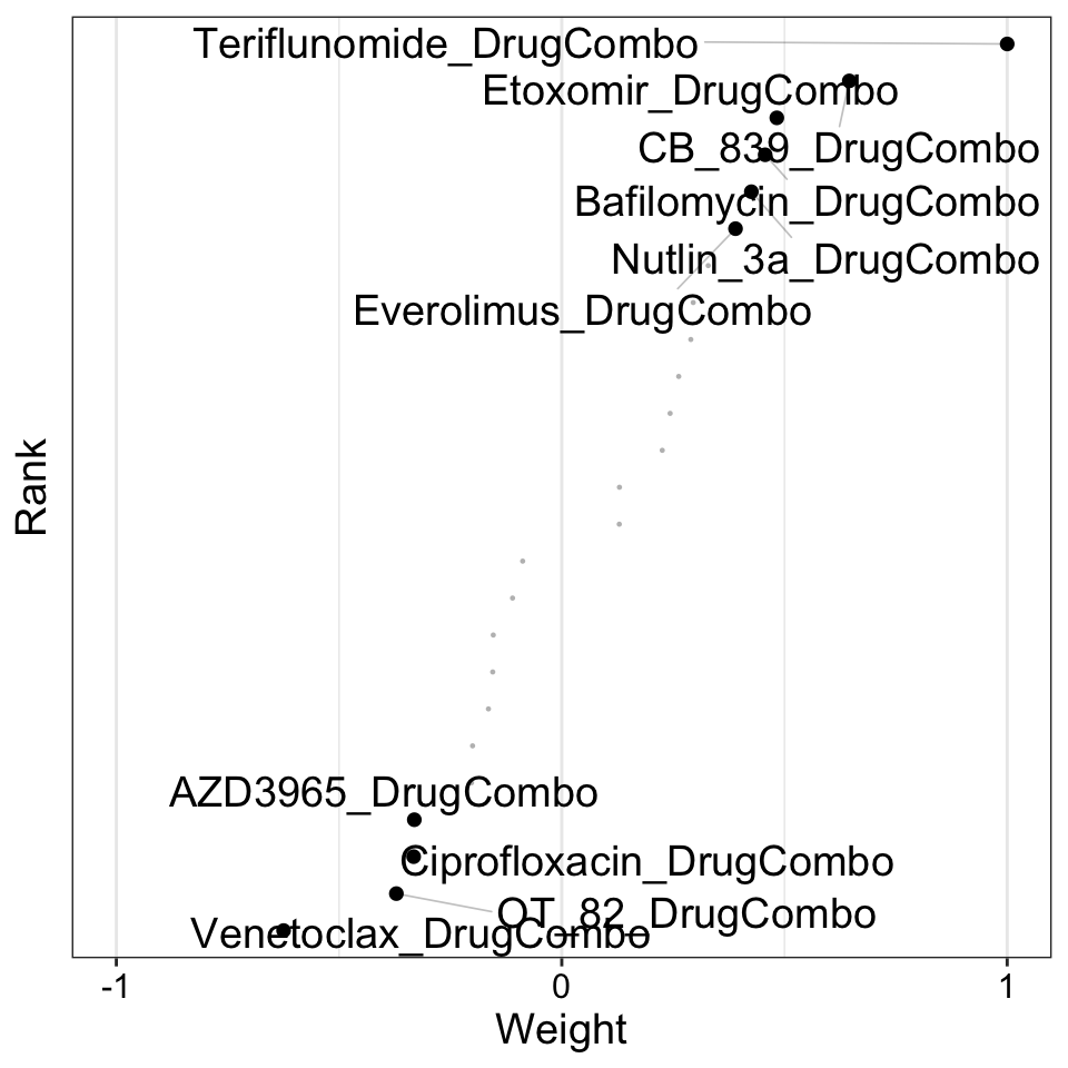
Weight of drug combo features on LF3
plot_weights(MOFAobject,
 view = "DrugCombo",
 factor = 3,
 nfeatures = 10,     # Top number of features to highlight
 scale = T           # Scale weights from -1 to 1
)
Weight of protein features
plot_weights(MOFAobject,
 view = "Protein",
 factor = 3,
 nfeatures = 10,     # Top number of features to highlight
 scale = T           # Scale weights from -1 to 1
)
Weight of metabolites features
plot_weights(MOFAobject,
 view = "Metabolite",
 factor =3,
 nfeatures = 10,     # Top number of features to highlight
 scale = T           # Scale weights from -1 to 1
)
Focus on F4
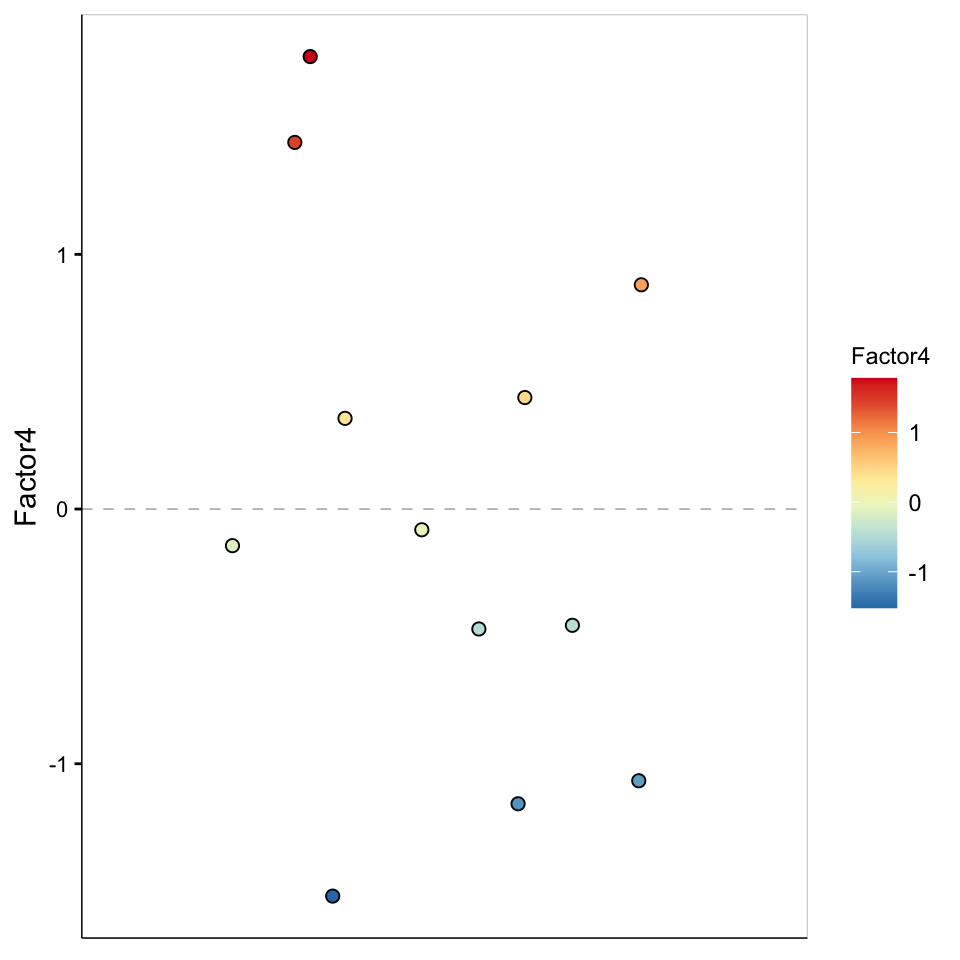
Factor 4 values
plot_factor(MOFAobject,
  factors = 4,
  color_by = "Factor4"
)
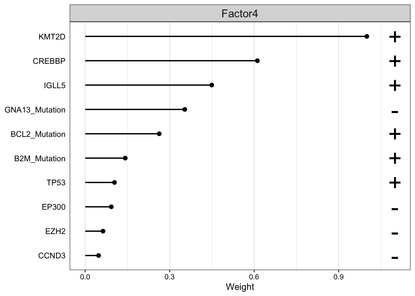
Weight of genomic features on LF4
plot_top_weights(MOFAobject,
 view = "Mutation",
 factor =4,
 nfeatures = 10,     # Top number of features to highlight
 scale = T           # Scale weights from -1 to 1
)
Weight of drug features on LF3
plot_weights(MOFAobject,
 view = "Drug",
 factor = 4,
 nfeatures = 10,     # Top number of features to highlight
 scale = T           # Scale weights from -1 to 1
)
Weight of drug combo features on LF3
plot_weights(MOFAobject,
 view = "DrugCombo",
 factor = 4,
 nfeatures = 10,     # Top number of features to highlight
 scale = T           # Scale weights from -1 to 1
)
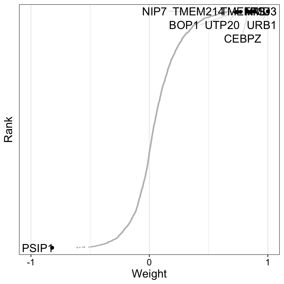
Weight of protein features
plot_weights(MOFAobject,
 view = "Protein",
 factor = 4,
 nfeatures = 10,     # Top number of features to highlight
 scale = T           # Scale weights from -1 to 1
)
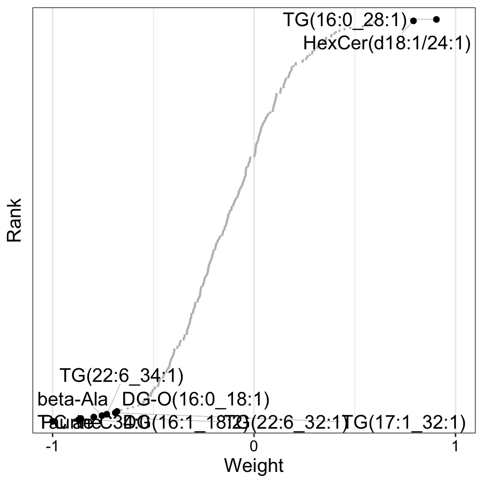
Weight of metabolites features
plot_weights(MOFAobject,
 view = "Metabolite",
 factor =4,
 nfeatures = 10,     # Top number of features to highlight
 scale = T           # Scale weights from -1 to 1
)
Focus on F1
facTab <- facMat %>% as_tibble(rownames = "factor") %>%
  pivot_longer(-factor) %>% filter(factor == "Factor1") %>%
  mutate(viab = drugMat["CHP",name]) %>%
  mutate(TP53 = geneMat["TP53",name]) %>%
  mutate(TP53 = ifelse(TP53==1, "Mut","WT"))
F1 versus CHP
ggplot(facTab, aes(x=value, y = viab)) +
  geom_point(aes(col  = TP53)) + geom_smooth(method = "lm", se = FALSE) +
  theme_bw() +
  theme(legend.position = c(0.8, 0.2)) +
  ylab("CHP response") + xlab("Factor 1")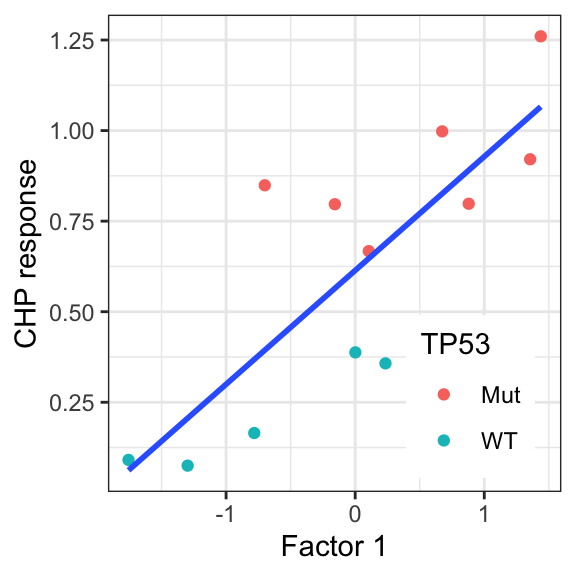
F1 versus TP53
ggplot(facTab, aes(x=TP53, y = value)) +
  geom_boxplot(width=0.5, aes(fill = TP53)) + geom_point() +
  theme_bw() +
  theme(legend.position = "none") +
  ylab("Factor 1")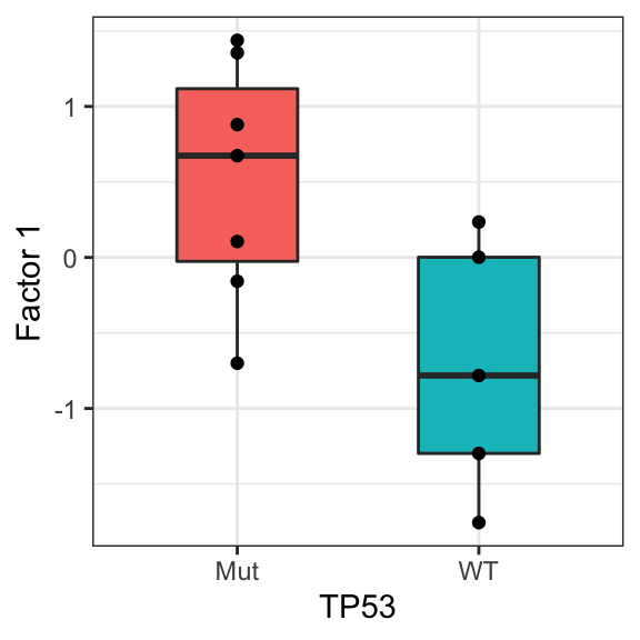
sessionInfo()R version 4.2.0 (2022-04-22)
Platform: x86_64-apple-darwin17.0 (64-bit)
Running under: macOS Big Sur/Monterey 10.16
Matrix products: default
BLAS: /Library/Frameworks/R.framework/Versions/4.2/Resources/lib/libRblas.0.dylib
LAPACK: /Library/Frameworks/R.framework/Versions/4.2/Resources/lib/libRlapack.dylib
locale:
[1] en_US.UTF-8/en_US.UTF-8/en_US.UTF-8/C/en_US.UTF-8/en_US.UTF-8
attached base packages:
[1] stats4 stats graphics grDevices utils datasets methods
[8] base
other attached packages:
[1] pheatmap_1.0.12 SummarizedExperiment_1.26.1
[3] Biobase_2.56.0 GenomicRanges_1.48.0
[5] GenomeInfoDb_1.32.2 IRanges_2.30.0
[7] S4Vectors_0.34.0 BiocGenerics_0.42.0
[9] MatrixGenerics_1.8.1 matrixStats_0.62.0
[11] forcats_0.5.1 stringr_1.4.0
[13] dplyr_1.0.9 purrr_0.3.4
[15] readr_2.1.2 tidyr_1.2.0
[17] tibble_3.1.8 ggplot2_3.3.6
[19] tidyverse_1.3.2 MOFA2_1.6.0
[21] jyluMisc_0.1.5
loaded via a namespace (and not attached):
[1] utf8_1.2.2 shinydashboard_0.7.2
[3] reticulate_1.25 tidyselect_1.1.2
[5] htmlwidgets_1.5.4 grid_4.2.0
[7] BiocParallel_1.30.3 Rtsne_0.16
[9] maxstat_0.7-25 munsell_0.5.0
[11] preprocessCore_1.58.0 codetools_0.2-18
[13] DT_0.23 withr_2.5.0
[15] colorspace_2.0-3 filelock_1.0.2
[17] highr_0.9 knitr_1.39
[19] rstudioapi_0.13 ggsignif_0.6.3
[21] labeling_0.4.2 git2r_0.30.1
[23] slam_0.1-50 GenomeInfoDbData_1.2.8
[25] KMsurv_0.1-5 farver_2.1.1
[27] rhdf5_2.40.0 rprojroot_2.0.3
[29] coda_0.19-4 basilisk_1.8.0
[31] vctrs_0.4.1 generics_0.1.3
[33] TH.data_1.1-1 xfun_0.31
[35] sets_1.0-21 R6_2.5.1
[37] reshape_0.8.9 bitops_1.0-7
[39] rhdf5filters_1.8.0 cachem_1.0.6
[41] fgsea_1.22.0 DelayedArray_0.22.0
[43] assertthat_0.2.1 promises_1.2.0.1
[45] scales_1.2.0 multcomp_1.4-19
[47] googlesheets4_1.0.0 gtable_0.3.0
[49] sandwich_3.0-2 workflowr_1.7.0
[51] rlang_1.0.4 GlobalOptions_0.1.2
[53] splines_4.2.0 rstatix_0.7.0
[55] gargle_1.2.0 broom_1.0.0
[57] yaml_2.3.5 reshape2_1.4.4
[59] abind_1.4-5 modelr_0.1.8
[61] backports_1.4.1 httpuv_1.6.5
[63] tools_4.2.0 relations_0.6-12
[65] statnet.common_4.6.0 ellipsis_0.3.2
[67] gplots_3.1.3 jquerylib_0.1.4
[69] RColorBrewer_1.1-3 ggdendro_0.1.23
[71] proxy_0.4-27 MultiAssayExperiment_1.22.0
[73] Rcpp_1.0.9 plyr_1.8.7
[75] visNetwork_2.1.0 zlibbioc_1.42.0
[77] RCurl_1.98-1.7 basilisk.utils_1.8.0
[79] ggpubr_0.4.0 viridis_0.6.2
[81] cowplot_1.1.1 zoo_1.8-10
[83] haven_2.5.0 ggrepel_0.9.1
[85] cluster_2.1.3 exactRankTests_0.8-35
[87] fs_1.5.2 magrittr_2.0.3
[89] data.table_1.14.2 PhosR_1.6.0
[91] circlize_0.4.15 reprex_2.0.1
[93] survminer_0.4.9 pcaMethods_1.88.0
[95] googledrive_2.0.0 mvtnorm_1.1-3
[97] hms_1.1.1 shinyjs_2.1.0
[99] mime_0.12 evaluate_0.15
[101] xtable_1.8-4 readxl_1.4.0
[103] gridExtra_2.3 shape_1.4.6
[105] compiler_4.2.0 KernSmooth_2.23-20
[107] crayon_1.5.1 htmltools_0.5.3
[109] mgcv_1.8-40 later_1.3.0
[111] tzdb_0.3.0 lubridate_1.8.0
[113] DBI_1.1.3 corrplot_0.92
[115] dbplyr_2.2.1 MASS_7.3-58
[117] Matrix_1.4-1 car_3.1-0
[119] cli_3.3.0 marray_1.74.0
[121] parallel_4.2.0 igraph_1.3.4
[123] pkgconfig_2.0.3 km.ci_0.5-6
[125] dir.expiry_1.4.0 piano_2.12.0
[127] xml2_1.3.3 bslib_0.4.0
[129] ruv_0.9.7.1 XVector_0.36.0
[131] drc_3.0-1 rvest_1.0.2
[133] digest_0.6.29 rmarkdown_2.14
[135] cellranger_1.1.0 fastmatch_1.1-3
[137] survMisc_0.5.6 dendextend_1.16.0
[139] uwot_0.1.11 shiny_1.7.2
[141] gtools_3.9.3 nlme_3.1-158
[143] lifecycle_1.0.1 jsonlite_1.8.0
[145] Rhdf5lib_1.18.2 network_1.17.2
[147] carData_3.0-5 viridisLite_0.4.0
[149] limma_3.52.2 fansi_1.0.3
[151] pillar_1.8.0 GGally_2.1.2
[153] lattice_0.20-45 fastmap_1.1.0
[155] httr_1.4.3 plotrix_3.8-2
[157] survival_3.3-1 glue_1.6.2
[159] png_0.1-7 class_7.3-20
[161] stringi_1.7.8 sass_0.4.2
[163] HDF5Array_1.24.1 caTools_1.18.2
[165] e1071_1.7-11