Compare the difference between TP53 mutational signature and Doxorubicine resistant signature to identify pathways related to Doxorubicine resistance
Junyan Lu
2022-08-12
Last updated: 2022-09-05
Checks: 4 2
Knit directory: combiDLBCL/analysis/
This reproducible R Markdown analysis was created with workflowr (version 1.7.0). The Checks tab describes the reproducibility checks that were applied when the results were created. The Past versions tab lists the development history.
Great job! The global environment was empty. Objects defined in the global environment can affect the analysis in your R Markdown file in unknown ways. For reproduciblity it’s best to always run the code in an empty environment.
The command set.seed(20220425) was run prior to running
the code in the R Markdown file. Setting a seed ensures that any results
that rely on randomness, e.g. subsampling or permutations, are
reproducible.
Great job! Recording the operating system, R version, and package versions is critical for reproducibility.
- unnamed-chunk-15
- unnamed-chunk-24
- unnamed-chunk-40
To ensure reproducibility of the results, delete the cache directory
TP53_analysis_allCellline_cache and re-run the analysis. To
have workflowr automatically delete the cache directory prior to
building the file, set delete_cache = TRUE when running
wflow_build() or wflow_publish().
Great job! Using relative paths to the files within your workflowr project makes it easier to run your code on other machines.
Tracking code development and connecting the code version to the
results is critical for reproducibility. To start using Git, open the
Terminal and type git init in your project directory.
This project is not being versioned with Git. To obtain the full
reproducibility benefits of using workflowr, please see
?wflow_start.
Load libraries and datasets
Compare Doxorubicine and CHP response
Pre-processing
Process the new screen data by Lea
load("../output/screenData.RData")
chpTab <- filter(screenData, Drug_A %in% "DMSO", Drug_B == "CHP", Plate == "CHP:Pola") %>%
  mutate(Name = ifelse(Name %in% "Karpas1106p","Karpas-1106p",Name)) %>%
  group_by(Name, Drug_B, Drug_B.Conc) %>%
  summarise(normVal = mean(normVal, na.rm=TRUE)) %>%
  rename(Drug = Drug_B, conc = Drug_B.Conc) %>%
  group_by(Name, Drug) %>%
  summarise(auc = calcAUC(normVal, conc))
Process the old screen data by Tobias
load("../data/Screen.CL19.RData")
doxoTab <- filter(Screen.CL19, Drug %in% "Doxorubicine", TimePoint == "48 h", Name %in% chpTab$Name | str_detect(Entity, "DLBCL")) %>%
  dplyr::rename(normVal = Normalized, conc = Drug.Conc) %>%
  group_by(Name, Drug, conc) %>%
  summarise(normVal = mean(normVal, na.rm=TRUE)) %>%
  group_by(Name, Drug) %>%
  summarise(auc = calcAUC(normVal, conc))
Genomics
load("../data/SVs.RData")
geneSub <- SVs %>%
  filter(Name %in% c(chpTab$Name, doxoTab$Name))
Overlapped cell liens
cellTab <- bind_rows(tibble(screen = "CHP", cell = unique(chpTab$Name)),
tibble(screen = "Doxo", cell = unique(doxoTab$Name)),
tibble(screen = "Gene", cell = unique(geneSub$Name)))
ggplot(cellTab, aes(x=cell, y=screen)) +
geom_tile(fill = "darkgreen", col = "grey50") +
theme_light() +
theme(axis.text.x = element_text(angle = 90, hjust=1, vjust=0.5))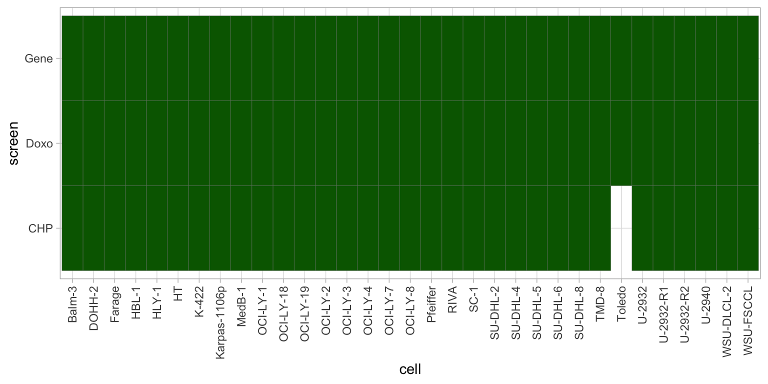 All the screened cell lines have genomic information.
Some cell lines screened by Lea are not DLBCL cell lines
nonDL <- filter(Screen.CL19, Name %in% cellTab$cell) %>%
  filter(!str_detect(Entity,"DLBCL")) %>%
  distinct(Name, Entity)
nonDL
# A tibble: 6 × 2
Name Entity
<chr> <chr>
1 Farage PMBL
2 U-2940 PMBL
3 MedB-1 PMBL
4 WSU-FSCCL FL
5 SC-1 FL
6 Karpas-1106p PMBL Those will be still used in this analysis.
Correlation of AUC
plotTab <- bind_rows(chpTab, doxoTab) %>%
  pivot_wider(names_from = Drug, values_from = auc) %>%
  mutate(missing = ifelse(is.na(CHP) | is.na(Doxorubicine), "yes","no")) %>%
  mutate(CHP = replace_na(CHP,0), Doxorubicine = replace_na(Doxorubicine,0))

ggplot(plotTab, aes(x=CHP, y=Doxorubicine)) +
  geom_point(aes(col = missing)) +
  ggrepel::geom_text_repel(aes(label = Name)) +
  geom_smooth(method = "lm")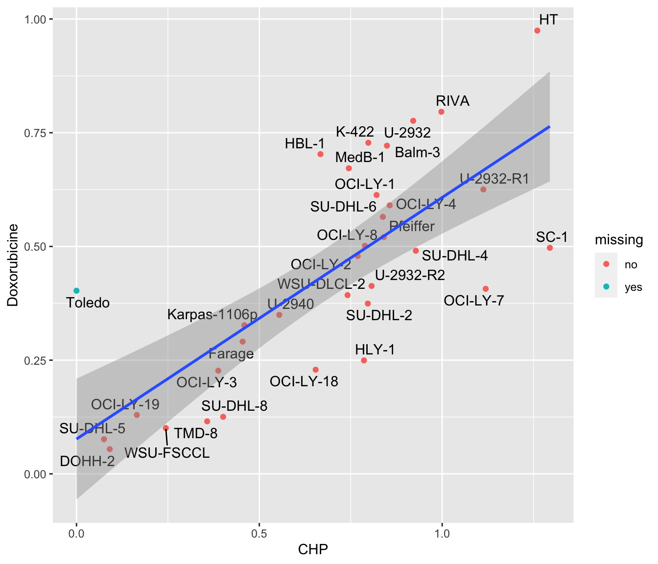
Examine the TP53 mutational status of DLBCL cell lines
tp53Tab <- filter(SVs, Gene == "TP53", Name %in% doxoTab$Name, Classification != "synonymous") %>%
  distinct(Name, Position, .keep_all = TRUE)
tp53Tab %>% DT::datatable()
Correlation of AUC, colored by TP53 mutation status
plotTab <- bind_rows(chpTab, doxoTab) %>%
pivot_wider(names_from = Drug, values_from = auc) %>%
#filter(!is.na(Doxorubicine)) %>%
mutate(missing = ifelse(is.na(CHP) | is.na(Doxorubicine), "yes","no")) %>%
mutate(CHP = replace_na(CHP,0), Doxorubicine = replace_na(Doxorubicine,0)) %>%
left_join(distinct(tp53Tab, Name, Classification), by = "Name") %>%
mutate(TP53 = ifelse(is.na(Classification), "WT", Classification))
ggplot(plotTab, aes(x=CHP, y=Doxorubicine)) +
geom_point(aes(col = TP53, shape = missing)) +
ggrepel::geom_text_repel(aes(label = Name)) +
geom_smooth(method = "lm")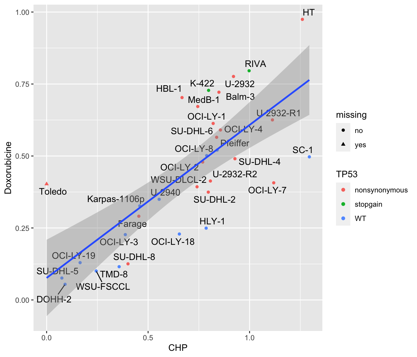 Based on this article, https://www.ncbi.nlm.nih.gov/pmc/articles/PMC3094765/,
Pfeiffer has mutated/deleted TP53.
Based on this article, https://www.ncbi.nlm.nih.gov/pmc/articles/PMC3094765/,
Pfeiffer has mutated/deleted TP53.
Based on this article, https://www.ncbi.nlm.nih.gov/pmc/articles/PMC6882812/,
OCI-LY-8 cell line also has mutated TP53.
Based on database, https://web.expasy.org/cellosaurus/CVCL_2207, SU-DHL-8, indeed has two TP53 mutations: Tyr234Asn and Arg249Gly (a known hotspot mutation).
There are not so much information about the TP53 status of Farage and SC-, we will just use the sequencing information.
Created a new TP53 mutational status table based on sequencing and prior knowledge.
tp53MutTab <- doxoTab %>% distinct(Name) %>%
  mutate(status = ifelse(Name %in% tp53Tab$Name,"Mut","WT")) %>%
  mutate(status = ifelse(Name %in% c("Pfeiffer", "OCI-LY-8"),"Mut",status)) %>%
  mutate(status = factor(status, levels = c("WT","Mut")))
Also add a column indicate sensitivity, it’s consistent with TP53 mutational status, except for SU-DHL-8
tp53MutTab <- mutate(tp53MutTab, doxoRes = ifelse(status == "Mut", "resistant","sensitive")) %>%
  mutate(doxoRes = case_when(Name %in% c("Farage","SU-DHL-8") ~ "sensitive",
                             Name %in% c("SC-1") ~ "resistant",
                             TRUE ~ doxoRes)) %>%
  #mutate(doxoRes = ifelse(Name == "SU-DHL-8","sensitive",doxoRes)) %>%
  mutate(doxoRes = factor(doxoRes, levels = c("sensitive","resistant")))
Association with proteomics
Preprocessing proteomic data from SMART-CARE
Normalization (already performed by Thomas)
protData <- readRDS("../data/SC005_SummarizedExperiment_proteomics.RDS")

#select baseline samples
protData <- protData[, protData$cell.line %in% tp53MutTab$Name]
protMat <- assay(protData)

#original
boxplot(protMat)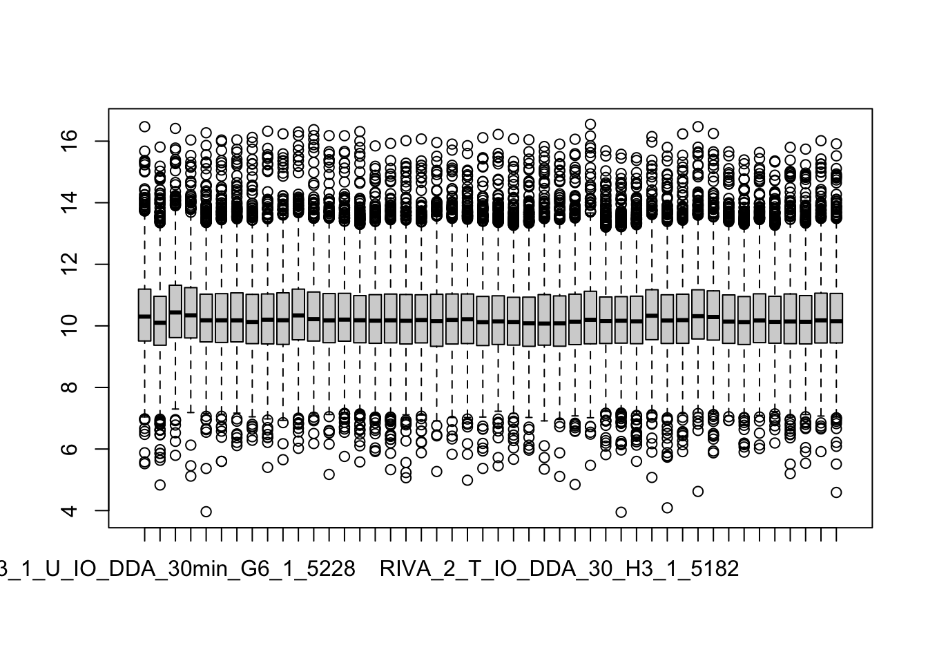
#median normalized
#protMatNorm <- PhosR::medianScaling(protMat, scale = FALSE)
#boxplot(protMatNorm)
protNorm <- protData
#assay(protNorm) <- protMatNorm
assayNames(protNorm) <- "norm"
dim(protNorm)
[1] 2643 46Average technical replicates for each cell line
protTab <- jyluMisc::sumToTidy(protNorm) %>%
  group_by(cell.line, rowID, Gene_name, condition) %>%
  summarise(count = mean(norm, na.rm=TRUE)) %>%
  dplyr::rename(symbol = Gene_name, cellLine = cell.line) %>%
  mutate(colID = paste0(cellLine,"_", condition)) %>%
  ungroup()

protAll <- jyluMisc::tidyToSum(protTab, rowID = "rowID", colID = "colID",
                     values = "count", annoRow = "symbol",
                     annoCol = c("condition", "cellLine"))

#add additional annotations
protAll$TP53 <- tp53MutTab[match(protAll$cellLine, tp53MutTab$Name),]$status
protAll$doxoRes <- tp53MutTab[match(protAll$cellLine, tp53MutTab$Name),]$doxoRes

#remove uncessary samples and records
protAll <- protAll[!rowData(protAll)$symbol %in% c("",NA), !is.na(protAll$TP53)]
dim(protAll)
[1] 2641 24colData(protAll) %>% data.frame() %>% DT::datatable()Differential expression in Baseline (Untreated) condition
protSub <- protAll[,protAll$condition == "U"]Differential protein expression using proDA
protMat <- assay(protSub)
fit <- proDA(protMat, design = ~ TP53,
             col_data = colData(protSub))

resTab <- test_diff(fit, contrast = "TP53Mut") %>%
  arrange(pval) %>%
  mutate(symbol = rowData(protSub[name,])$symbol)

resTab.base.smart <- resTab #for later comparison with Tobias data
Warning: The above code chunk cached its results, but
it won’t be re-run if previous chunks it depends on are updated. If you
need to use caching, it is highly recommended to also set
knitr::opts_chunk$set(autodep = TRUE) at the top of the
file (in a chunk that is not cached). Alternatively, you can customize
the option dependson for each individual chunk that is
cached. Using either autodep or dependson will
remove this warning. See the
knitr cache options for more details.
hist(resTab$pval)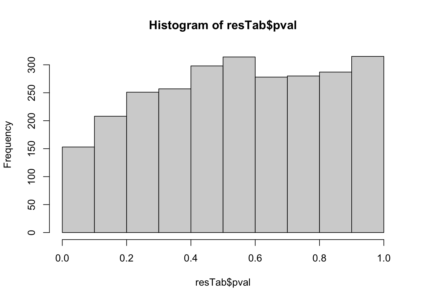 Not strong difference
Proteins with p-value < 0.05
resTab.sig <- filter(resTab, pval < 0.05)
resTab.sig %>% select(symbol, pval, adj_pval, diff) %>%
  mutate_if(is.numeric, formatC, digits=1) %>%
  DT::datatable()
Plot top 9 examples
pList <- lapply(seq(9), function(i) {
  rec <- resTab.sig[i,]
  plotTab <- tibble(expr = protMat[rec$name,],
                    doxoRes = protSub$doxoRes,
                    TP53 = protSub$TP53,
                    Name = colnames(protSub))
  ggplot(plotTab, aes(x=TP53, y=expr)) +
    geom_boxplot(outlier.shape = NA) +
    geom_point(aes(color = doxoRes), size=3) +
    ggrepel::geom_text_repel(aes(label = Name)) +
    ggtitle(rec$symbol) +
    theme_bw()
})

cowplot::plot_grid(plotlist = pList,ncol=3)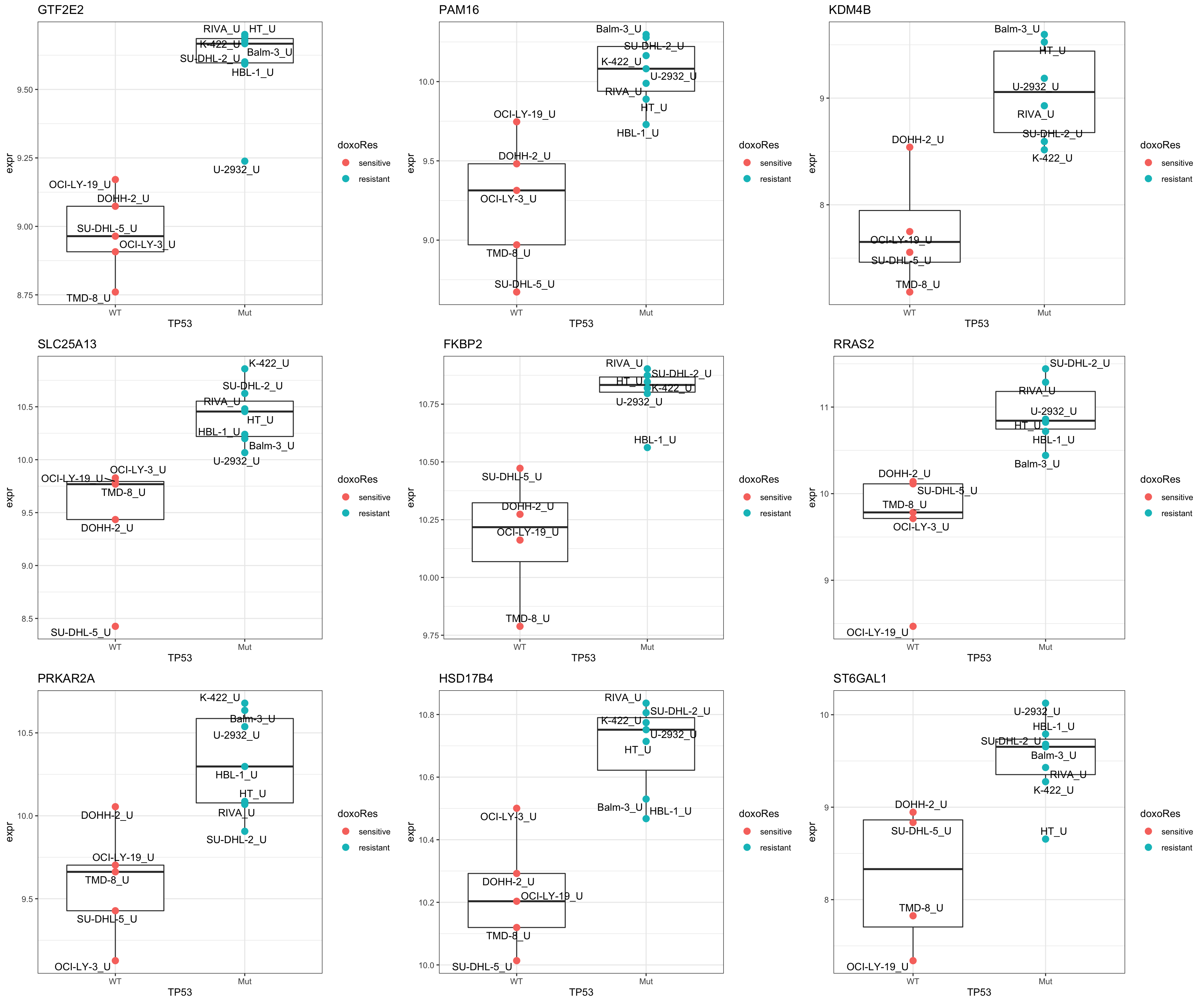
Enrichment analysis
gmts = list(H= "../data/gmts/h.all.v6.2.symbols.gmt",
            KEGG = "../data/gmts/c2.cp.kegg.v6.2.symbols.gmt",
            C6 = "../data/gmts/c6.all.v6.2.symbols.gmt")
inputTab <- resTab %>% filter(pval < 0.1) %>%
  distinct(symbol, .keep_all = TRUE) %>%
  select(symbol, t_statistic) %>% data.frame() %>% column_to_rownames("symbol")
enRes <- list()
enRes[["Hallmark"]] <- runGSEA(inputTab, gmts$H, "page")
enRes[["KEGG"]] <- runGSEA(inputTab, gmts$KEGG,"page")
enRes[["Perturbation"]] <- runGSEA(inputTab, gmts$C6,"page")
p <- jyluMisc::plotEnrichmentBar(enRes, pCut =0.05, ifFDR= FALSE)
cowplot::plot_grid(p)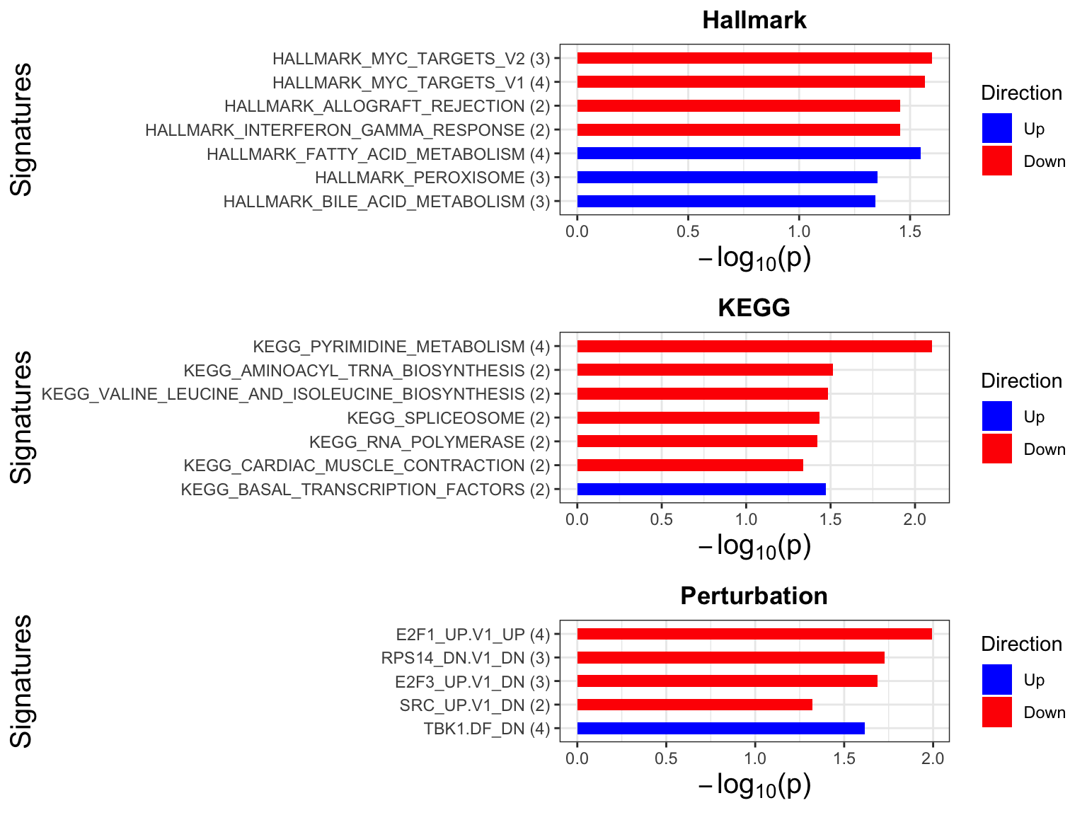
Focus on proteins from Fatty acid metabolism pathway
geneList <- piano::loadGSC(gmts$H)$gsc$HALLMARK_FATTY_ACID_METABOLISM
plotGene <- filter(filter(resTab, pval <= 0.1), symbol%in% geneList )
pList <- lapply(seq(nrow(plotGene)), function(i) {
  rec <- plotGene[i,]
  plotTab <- tibble(expr = protMat[rec$name,],
                    TP53 = protSub$TP53,
                    doxoRes = protSub$doxoRes)
  ggplot(plotTab, aes(x=TP53, y=expr)) +
    geom_boxplot(outlier.shape = NA) +
    ggbeeswarm::geom_quasirandom(aes(color = doxoRes), size=3) +
    ggtitle(rec$symbol) +
    theme_bw()
})

cowplot::plot_grid(plotlist = pList,ncol=3)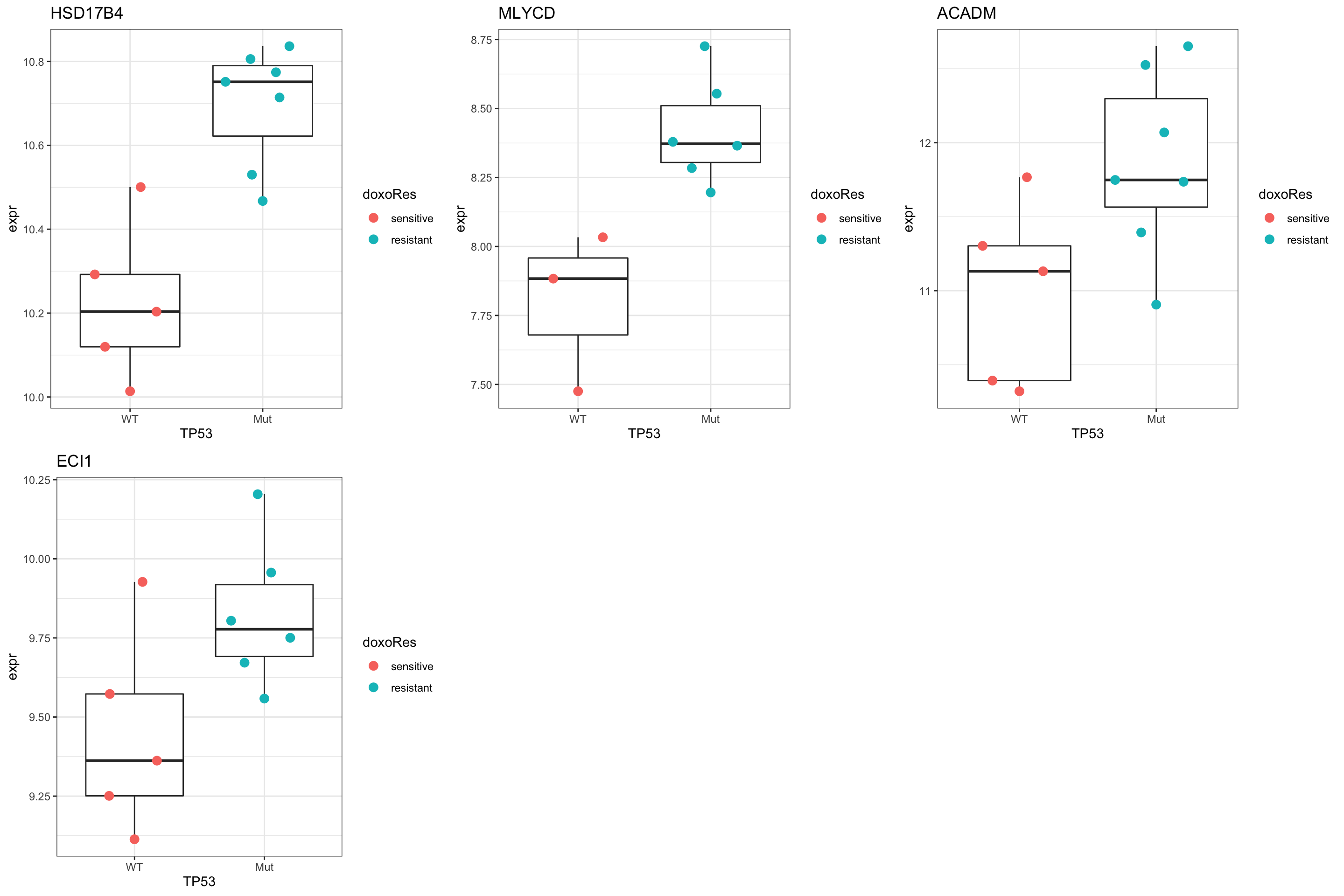
Focus on proteins from HALLMARK_PEROXISOME
geneList <- piano::loadGSC(gmts$H)$gsc$HALLMARK_PEROXISOME
plotGene <- filter(filter(resTab, pval <= 0.1), symbol%in% geneList )
pList <- lapply(seq(nrow(plotGene)), function(i) {
  rec <- plotGene[i,]
  plotTab <- tibble(expr = protMat[rec$name,],
                    TP53 = protSub$TP53,
                    doxoRes = protSub$doxoRes)
  ggplot(plotTab, aes(x=TP53, y=expr)) +
    geom_boxplot(outlier.shape = NA) +
    ggbeeswarm::geom_quasirandom(aes(color = doxoRes), size=3) +
    ggtitle(rec$symbol) +
    theme_bw()
})

cowplot::plot_grid(plotlist = pList,ncol=3)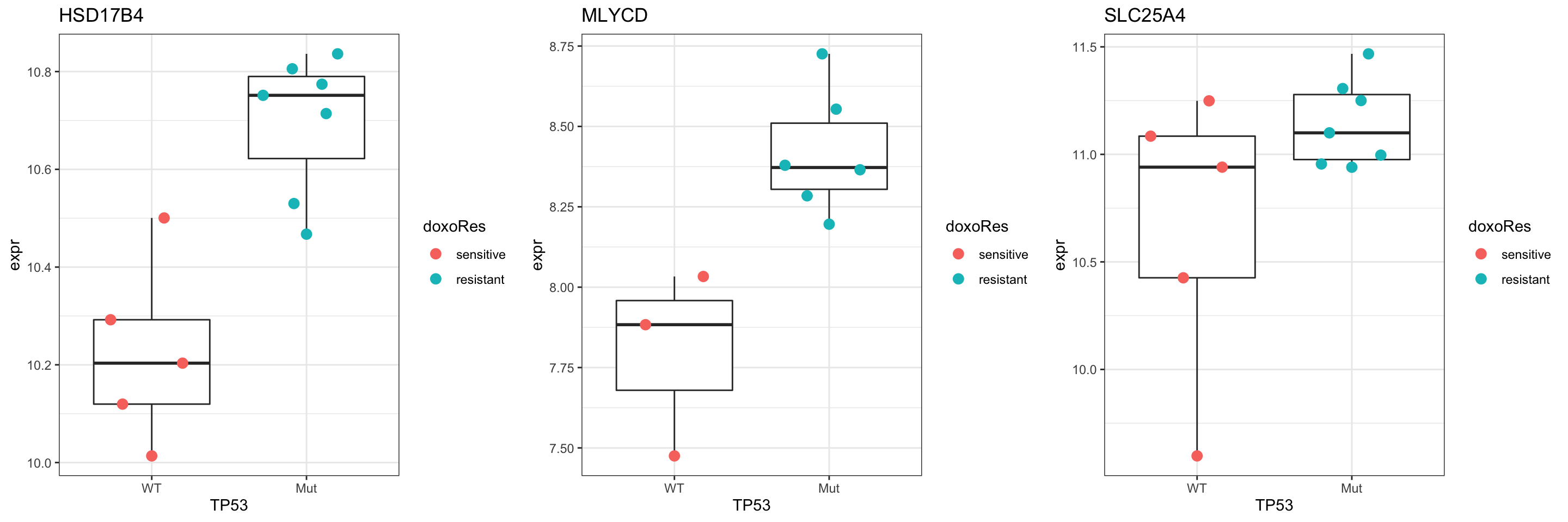
How about CPT1A?
plotGene <- filter(resTab, symbol%in% "CPT1A")
pList <- lapply(seq(nrow(plotGene)), function(i) {
  rec <- plotGene[i,]
  plotTab <- tibble(expr = protMat[rec$name,],
                    TP53 = protSub$TP53,
                    doxoRes = protSub$doxoRes)
  ggplot(plotTab, aes(x=TP53, y=expr)) +
    geom_boxplot(outlier.shape = NA) +
    ggbeeswarm::geom_quasirandom(aes(color = doxoRes), size=3) +
    ggtitle(rec$symbol) +
    theme_bw()
})

cowplot::plot_grid(plotlist = pList,ncol=1)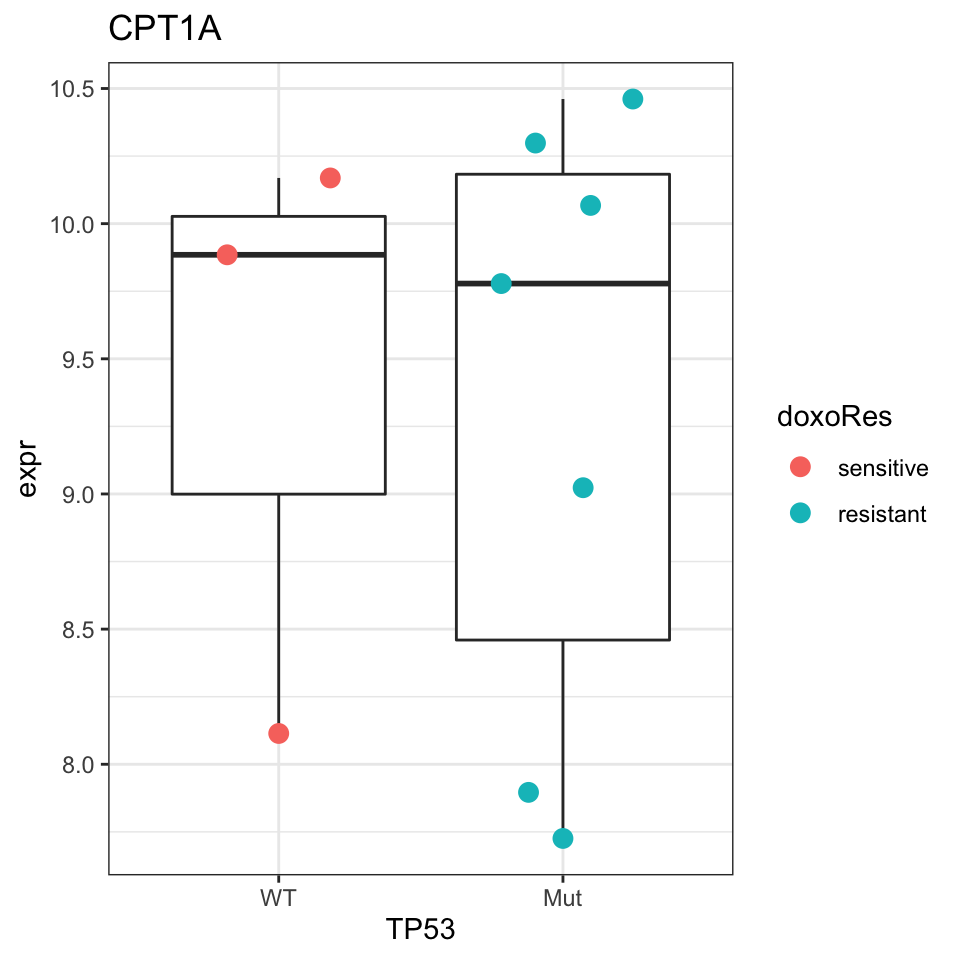
Differential expression between treated and untreated
protSub <- protAllDifferential protein expression using proDA
protMat <- assay(protSub)
fit <- proDA(protMat, design = ~ cellLine + condition,
             col_data = colData(protSub))

resTab <- test_diff(fit, contrast = "conditionT") %>%
  arrange(pval) %>%
  mutate(symbol = rowData(protSub[name,])$symbol)
Warning: The above code chunk cached its results, but
it won’t be re-run if previous chunks it depends on are updated. If you
need to use caching, it is highly recommended to also set
knitr::opts_chunk$set(autodep = TRUE) at the top of the
file (in a chunk that is not cached). Alternatively, you can customize
the option dependson for each individual chunk that is
cached. Using either autodep or dependson will
remove this warning. See the
knitr cache options for more details.
hist(resTab$pval)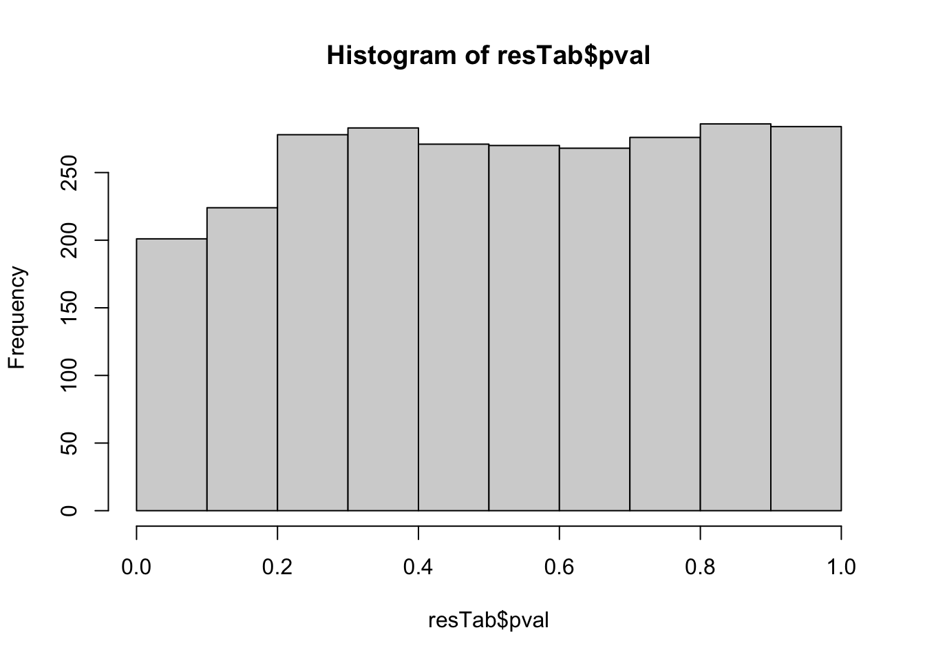 Not strong difference
Proteins with p-value < 0.05
resTab.sig <- filter(resTab, pval < 0.05)
resTab.sig %>% select(symbol, pval, adj_pval, diff) %>%
  mutate_if(is.numeric, formatC, digits=1) %>%
  DT::datatable()
Plot top 9 examples
pList <- lapply(seq(9), function(i) {
  rec <- resTab.sig[i,]
  plotTab <- tibble(expr = protMat[rec$name,],
                    TP53 = protSub$TP53,
                    Name = protSub$cellLine,
                    condition = protSub$condition)
  ggplot(plotTab, aes(x=condition, y=expr)) +
    geom_boxplot(outlier.shape = NA) +
    geom_point(aes(color = TP53), size=3) +
    geom_line(aes(group = Name), linetype = "dotted") +
    ggrepel::geom_text_repel(aes(label = Name)) +
    ggtitle(rec$symbol) +
    theme_bw()
})

cowplot::plot_grid(plotlist = pList,ncol=3)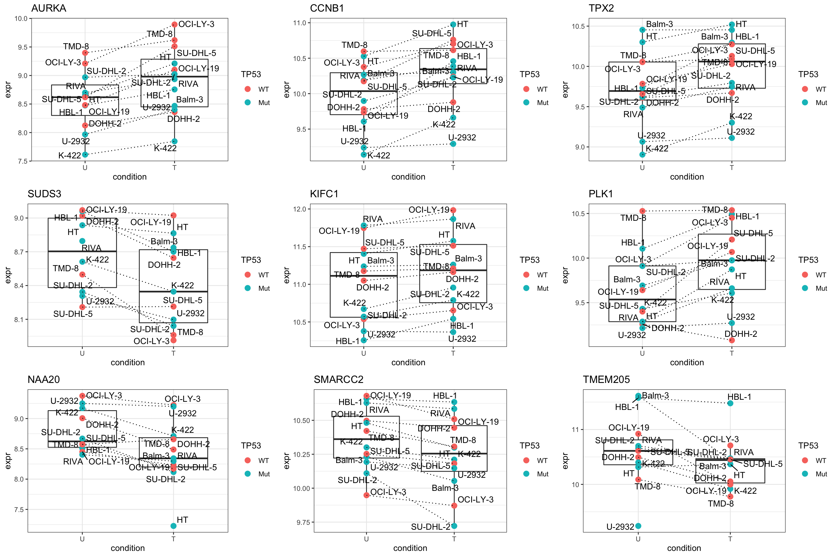
Enrichment analysis
gmts = list(H= "../data/gmts/h.all.v6.2.symbols.gmt",
            KEGG = "../data/gmts/c2.cp.kegg.v6.2.symbols.gmt",
            C6 = "../data/gmts/c6.all.v6.2.symbols.gmt")
inputTab <- resTab %>% filter(pval < 0.1) %>%
  distinct(symbol, .keep_all = TRUE) %>%
  select(symbol, t_statistic) %>% data.frame() %>% column_to_rownames("symbol")
enRes <- list()
enRes[["Hallmark"]] <- runGSEA(inputTab, gmts$H, "page")
enRes[["KEGG"]] <- runGSEA(inputTab, gmts$KEGG,"page")
enRes[["Perturbation"]] <- runGSEA(inputTab, gmts$C6,"page")
p <- jyluMisc::plotEnrichmentBar(enRes, pCut =0.05, ifFDR= FALSE)
cowplot::plot_grid(p)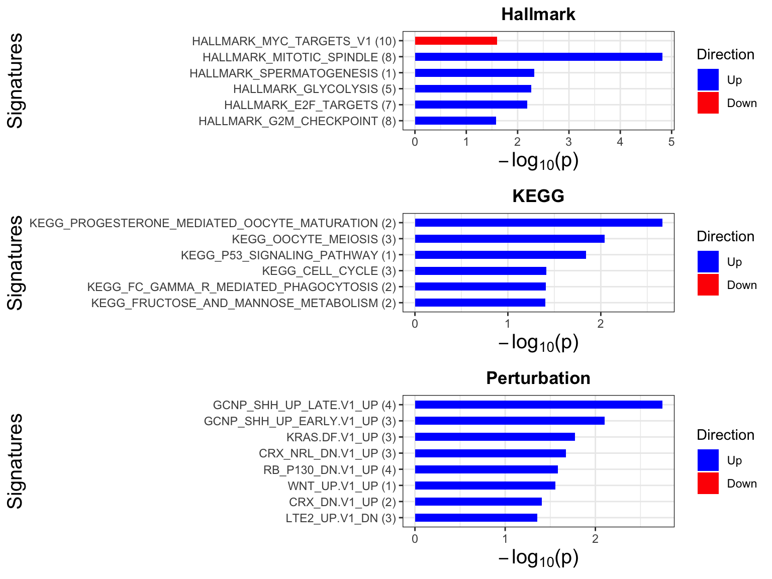
Interaction between treatment and sensitivity cluster
protSub <- protAllDifferential protein expression using proDA
protMat <- assay(protSub)
design <- model.matrix(~ 0 + condition*TP53, data = colData(protSub))
colnames(design) <- make.names(colnames(design))

cor <- duplicateCorrelation(protMat, design, block=protSub$cellLine)
#cor$consensus.correlation

fit <- lmFit(object=protMat, design=design, block=protSub$cellLine,
    correlation = cor$consensus.correlation, method = "ls")
fit2 <- eBayes(fit)
resTab  <- topTable(fit2, number = Inf, coef="conditionT.TP53Mut") %>%
  as_tibble(rownames = "name") %>%
  mutate(symbol = rowData(protSub[name,])$symbol) %>%
  dplyr::rename(pval = P.Value, adj_pval = adj.P.Val, diff = logFC, t_statistics = t)
hist(resTab$pval)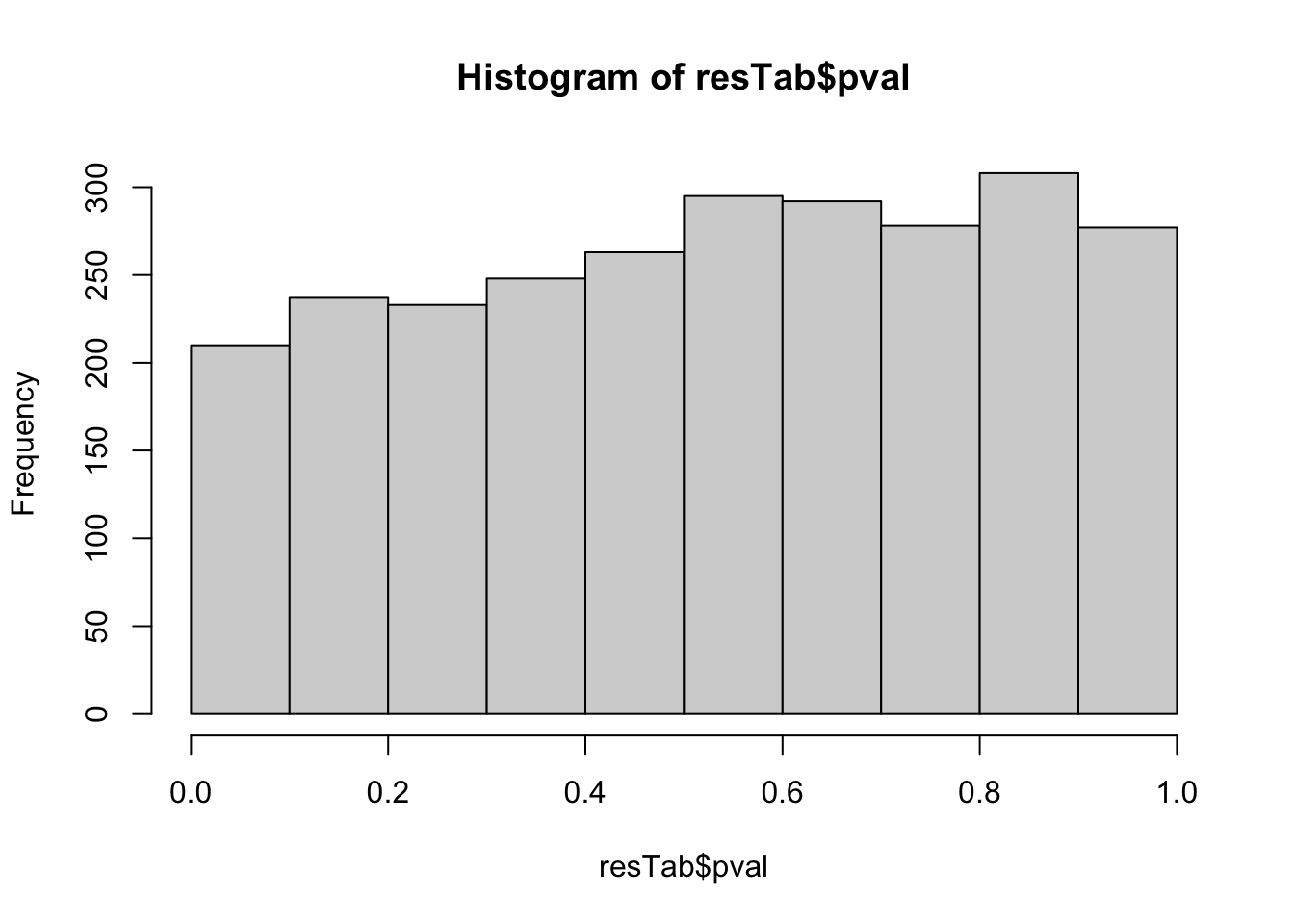 Not strong difference
Proteins with p-value < 0.05
resTab.sig <- filter(resTab, pval < 0.05)
resTab.sig %>% select(symbol, pval, adj_pval, diff) %>%
  mutate_if(is.numeric, formatC, digits=1) %>%
  DT::datatable()
Plot top 9 examples
pList <- lapply(seq(9), function(i) {
  rec <- resTab.sig[i,]
  plotTab <- tibble(expr = protMat[rec$name,],
                    TP53 = protSub$TP53,
                    Name = protSub$cellLine,
                    condition = protSub$condition)
  ggplot(plotTab, aes(x=condition, y=expr)) +
    geom_boxplot(outlier.shape = NA) +
    geom_point(aes(color = TP53), size=3) +
    geom_line(aes(group = Name), linetype = "dotted") +
    ggrepel::geom_text_repel(aes(label = Name)) +
    ggtitle(rec$symbol) +
    theme_bw() +
    facet_wrap(~TP53)
})

cowplot::plot_grid(plotlist = pList,ncol=3)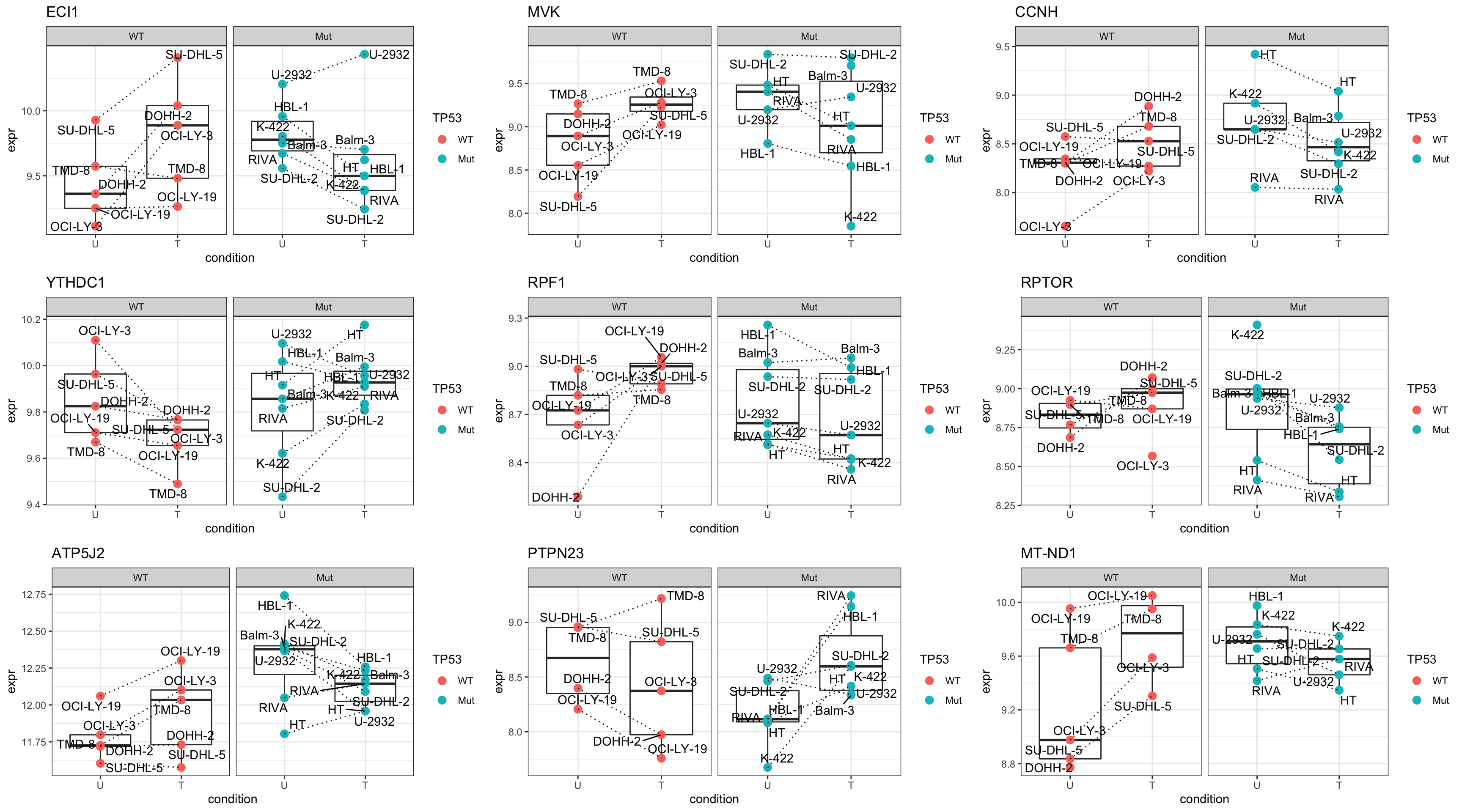
Enrichment analysis
gmts = list(H= "../data/gmts/h.all.v6.2.symbols.gmt",
KEGG = "../data/gmts/c2.cp.kegg.v6.2.symbols.gmt",
C6 = "../data/gmts/c6.all.v6.2.symbols.gmt")
inputTab <- resTab %>% filter(pval < 0.1) %>%
distinct(symbol, .keep_all = TRUE) %>%
select(symbol, t_statistics) %>% data.frame() %>% column_to_rownames("symbol")
enRes <- list()
enRes[["Hallmark"]] <- runGSEA(inputTab, gmts$H, "page")
enRes[["KEGG"]] <- runGSEA(inputTab, gmts$KEGG,"page")
enRes[["Perturbation"]] <- runGSEA(inputTab, gmts$C6,"page")
p <- jyluMisc::plotEnrichmentBar(enRes, pCut =0.05, ifFDR= FALSE)
cowplot::plot_grid(p)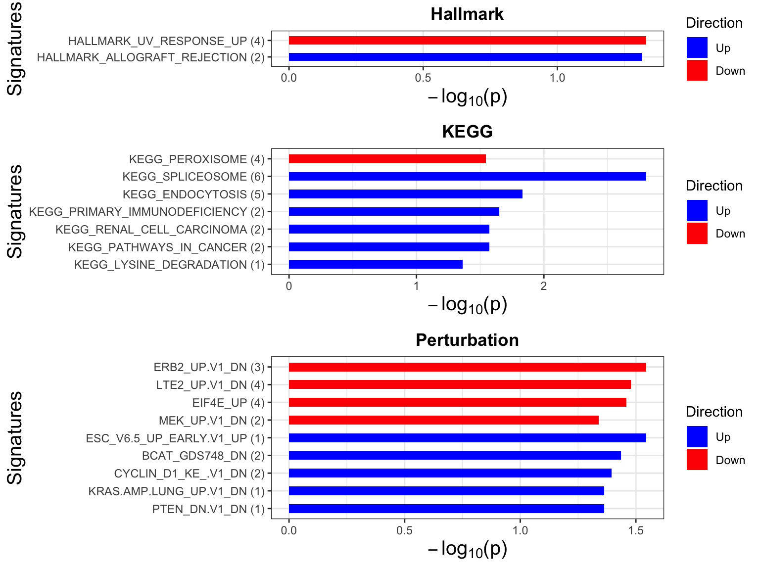 Focus on proteins from HALLMARK_PEROXISOME
geneList <- piano::loadGSC(gmts$H)$gsc$HALLMARK_PEROXISOME
plotGene <- filter(filter(resTab, pval <= 0.1), symbol%in% geneList )

pList <- lapply(seq(nrow(plotGene)), function(i) {
  rec <- plotGene[i,]
  plotTab <- tibble(expr = protMat[rec$name,],
                    TP53 = protSub$TP53,
                    Name = protSub$cellLine,
                    condition = protSub$condition)
  ggplot(plotTab, aes(x=condition, y=expr)) +
    geom_boxplot(outlier.shape = NA) +
    geom_point(aes(color = TP53), size=3) +
    geom_line(aes(group = Name), linetype = "dotted") +
    ggrepel::geom_text_repel(aes(label = Name)) +
    ggtitle(rec$name) +
    theme_bw() +
    facet_wrap(~TP53)
})

cowplot::plot_grid(plotlist = pList,ncol=3)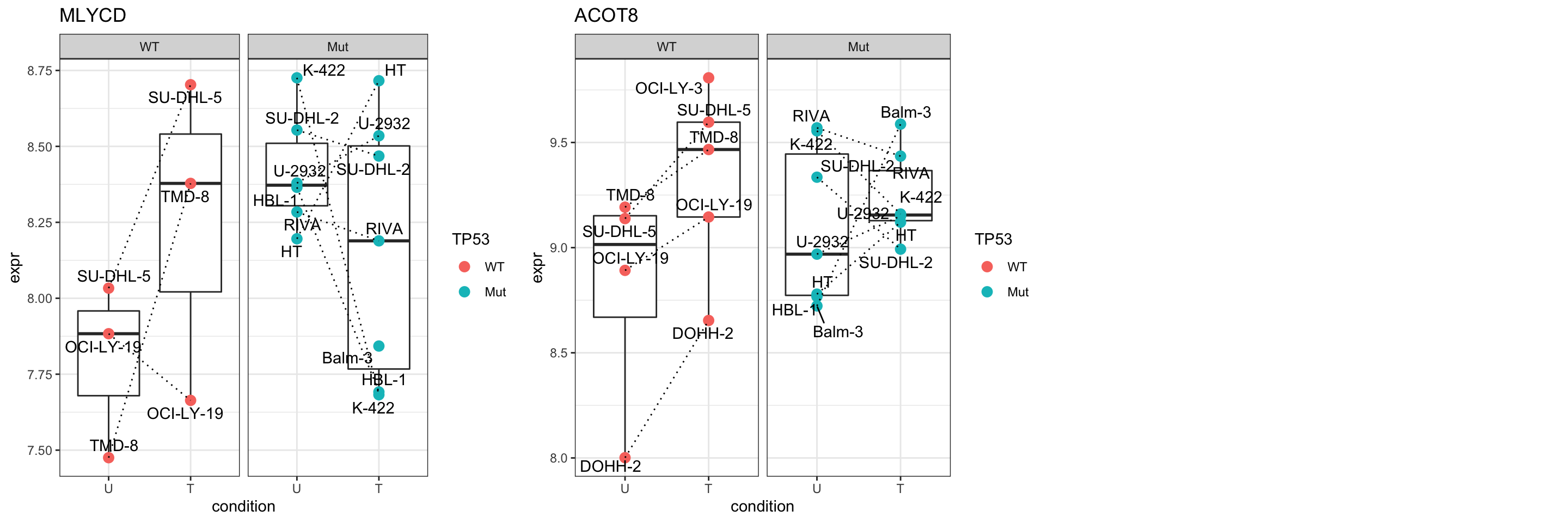
Baseline proteomics dataset from Tobias (EMBL dataset)
Data distribution
load("../data/ProtWide.RData")
ProtWide <- ProtWide[,colnames(ProtWide) %in% tp53MutTab$Name]
protMat <- ProtWide
dim(ProtWide)
[1] 4873 33Median normalization (not performed)
protMatNorm <- protMat
boxplot(protMatNorm)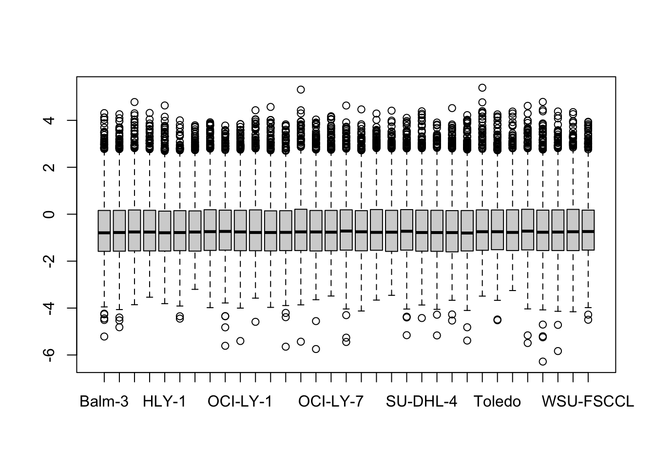
#protNorm <- protData
#assay(protNorm) <- protMatNorm
Create assay experiment object
protTab <- protMatNorm %>% as_tibble(rownames = "uniprotID") %>%
  pivot_longer(-uniprotID, names_to = "cellLine", values_to = "count") %>%
  mutate(TP53 = tp53MutTab[match(cellLine, tp53MutTab$Name),]$status,
         doxoRes = tp53MutTab[match(cellLine, tp53MutTab$Name),]$doxoRes,
         symbol = uniprotID) %>%
  filter(cellLine %in% tp53MutTab$Name,
         !symbol %in% c("",NA), !is.na(TP53))

protSub <- jyluMisc::tidyToSum(protTab, rowID = "uniprotID",colID = "cellLine",
                     values = "count", annoRow = "symbol", annoCol = c("TP53","doxoRes"))
#protSub$TP53 <- factor(colAnno[colnames(protSub),]$TP53)
colData(protSub) %>% as_tibble(rownames = "cellLine") %>%
DT::datatable()Identify proteins differentially expressed
Differential protein expression using proDA
protMat <- assay(protSub)
fit <- proDA(protMat, design = ~ TP53,
             col_data = colData(protSub))

resTab <- test_diff(fit, contrast = "TP53Mut") %>%
  arrange(pval) %>%
  mutate(symbol = rowData(protSub[name,])$symbol)

resTab.base.embl <- resTab
Warning: The above code chunk cached its results, but
it won’t be re-run if previous chunks it depends on are updated. If you
need to use caching, it is highly recommended to also set
knitr::opts_chunk$set(autodep = TRUE) at the top of the
file (in a chunk that is not cached). Alternatively, you can customize
the option dependson for each individual chunk that is
cached. Using either autodep or dependson will
remove this warning. See the
knitr cache options for more details.
hist(resTab$pval)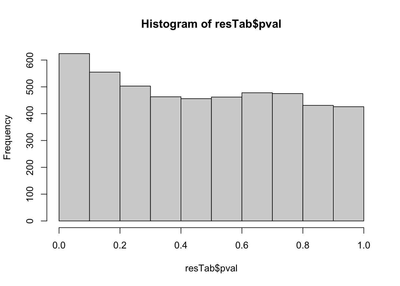 Stronger associations can be observed
Proteins with p-value < 0.05
resTab.sig <- filter(resTab, pval < 0.05)
resTab.sig %>% select(symbol, pval, adj_pval, diff) %>%
  mutate_if(is.numeric, formatC, digits=1) %>%
  DT::datatable()
Plot top 9 examples
pList <- lapply(seq(9), function(i) {
rec <- resTab.sig[i,]
plotTab <- tibble(expr = protMat[rec$name,],
TP53 = protSub$TP53,
Name = colnames(protSub),
doxoRes = protSub$doxoRes)
ggplot(plotTab, aes(x=TP53, y=expr)) +
geom_boxplot(outlier.shape = NA) +
geom_point(aes(color = doxoRes), size=3) +
ggrepel::geom_text_repel(aes(label = Name)) +
ggtitle(rec$symbol) +
theme_bw()
})
cowplot::plot_grid(plotlist = pList,ncol=3)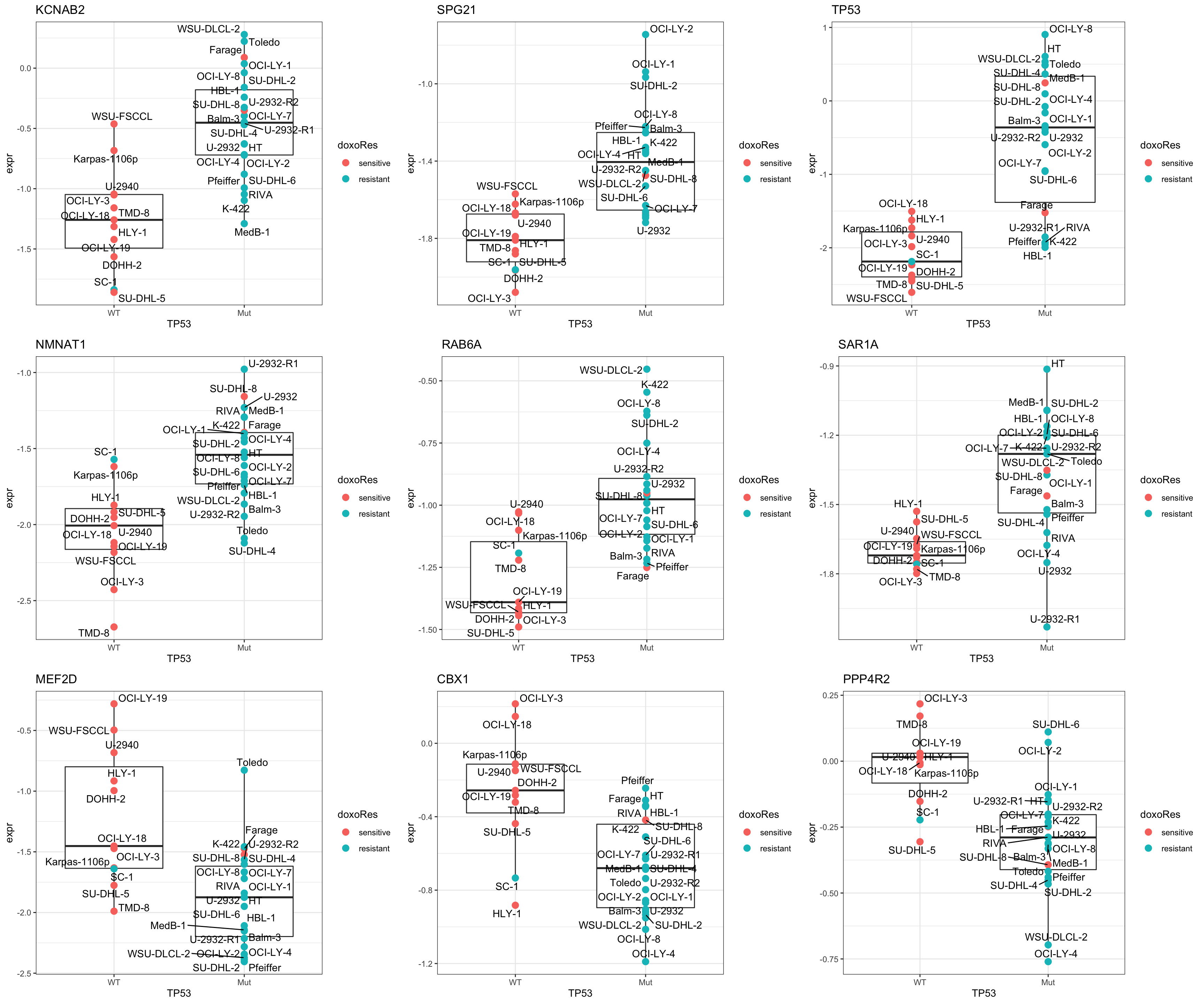 Overall DU-SHL-8 behaves similar to TP53 mutated samples
Enrichment analysis
gmts = list(H= "../data/gmts/h.all.v6.2.symbols.gmt",
            KEGG = "../data/gmts/c2.cp.kegg.v6.2.symbols.gmt",
            C6 = "../data/gmts/c6.all.v6.2.symbols.gmt")
inputTab <- resTab %>% filter(pval < 0.1) %>%
  distinct(symbol, .keep_all = TRUE) %>%
  select(symbol, t_statistic) %>% data.frame() %>% column_to_rownames("symbol")
enRes <- list()
enRes[["Hallmark"]] <- runGSEA(inputTab, gmts$H, "page")
enRes[["KEGG"]] <- runGSEA(inputTab, gmts$KEGG,"page")
enRes[["Perturbation"]] <- runGSEA(inputTab, gmts$C6,"page")
p <- jyluMisc::plotEnrichmentBar(enRes, pCut =0.1, ifFDR= TRUE)
[1] "No sets passed the criteria"cowplot::plot_grid(p)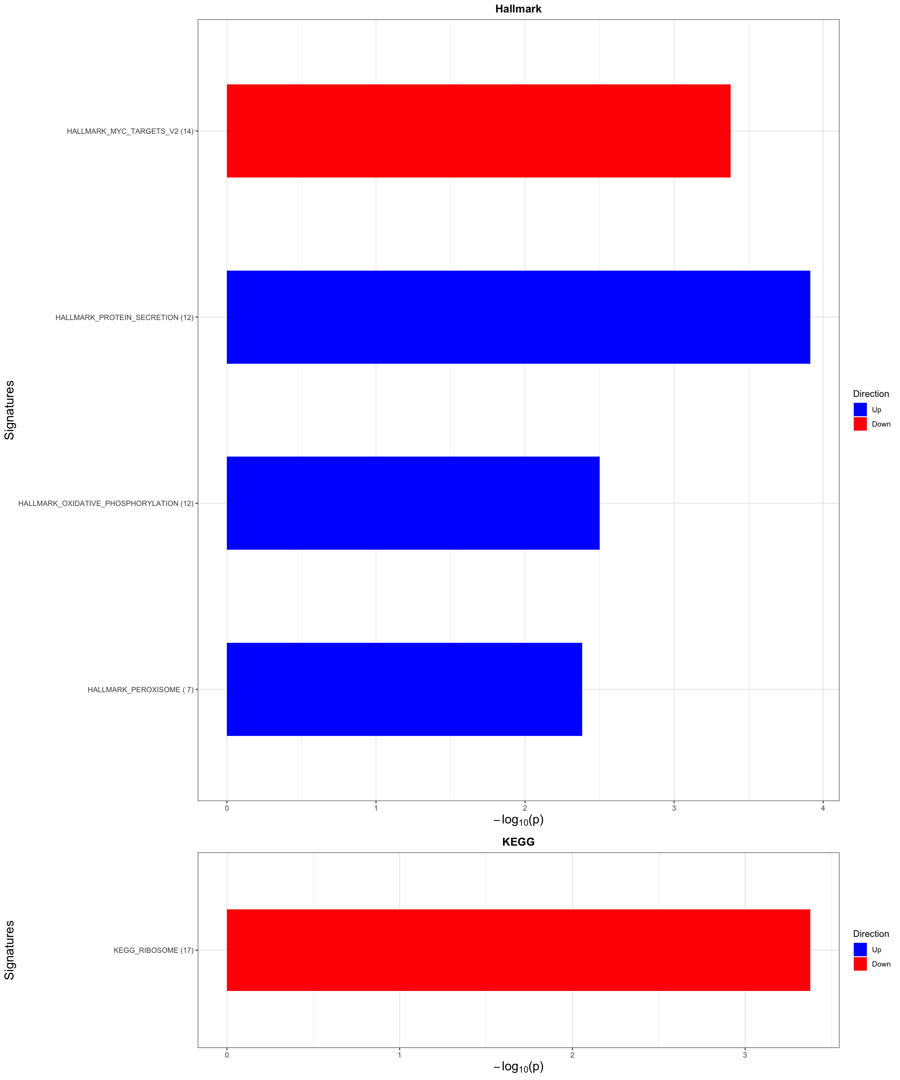
Focus on proteins from Fatty acid metabolism pathway
geneList <- piano::loadGSC(gmts$H)$gsc$HALLMARK_FATTY_ACID_METABOLISM
plotGene <- filter(filter(resTab, pval <= 0.05), symbol%in% geneList )
pList <- lapply(seq(nrow(plotGene)), function(i) {
rec <- plotGene[i,]
plotTab <- tibble(expr = protMat[rec$name,],
Name = colnames(protMat),
TP53 = protSub$TP53,
doxoRes = protSub$doxoRes)
ggplot(plotTab, aes(x=TP53, y=expr)) +
geom_boxplot(outlier.shape = NA) +
geom_point(aes(color = doxoRes), size=3) +
ggrepel::geom_text_repel(aes(label = Name)) +
ggtitle(rec$symbol) +
theme_bw()
})
cowplot::plot_grid(plotlist = pList,ncol=3)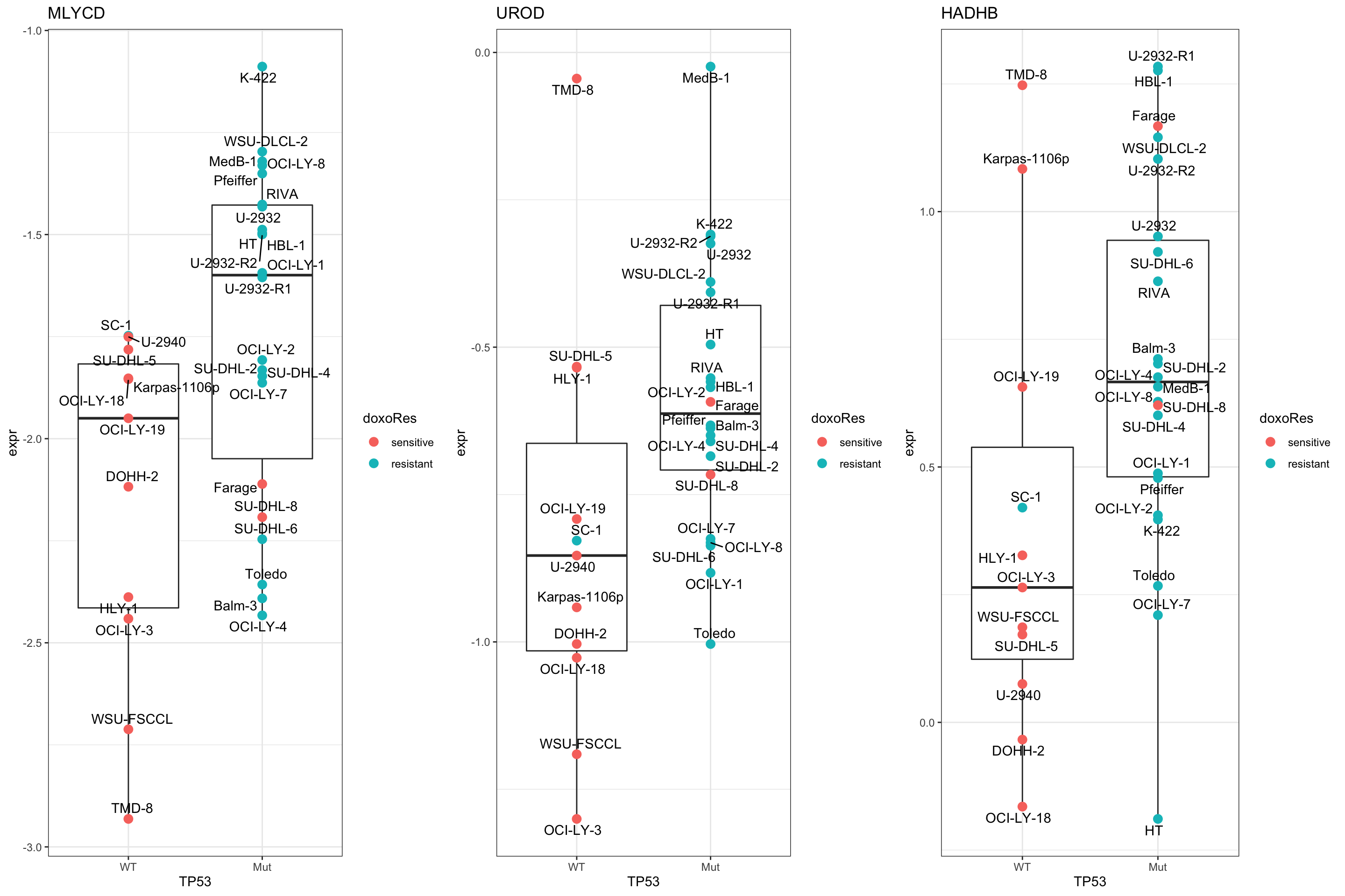 Focus on proteins from PEROXISOME pathway
geneList <- piano::loadGSC(gmts$H)$gsc$HALLMARK_PEROXISOME
plotGene <- filter(filter(resTab, pval <= 0.05), symbol%in% geneList )
pList <- lapply(seq(nrow(plotGene)), function(i) {
  rec <- plotGene[i,]
  plotTab <- tibble(expr = protMat[rec$name,],
                    Name = colnames(protMat),
                    TP53 = protSub$TP53,
                    doxoRes = protSub$doxoRes)
  ggplot(plotTab, aes(x=TP53, y=expr)) +
    geom_boxplot(outlier.shape = NA) +
    geom_point(aes(color = doxoRes), size=3) +
    ggrepel::geom_text_repel(aes(label = Name)) +
    ggtitle(rec$symbol) +
    theme_bw()
})

cowplot::plot_grid(plotlist = pList,ncol=3)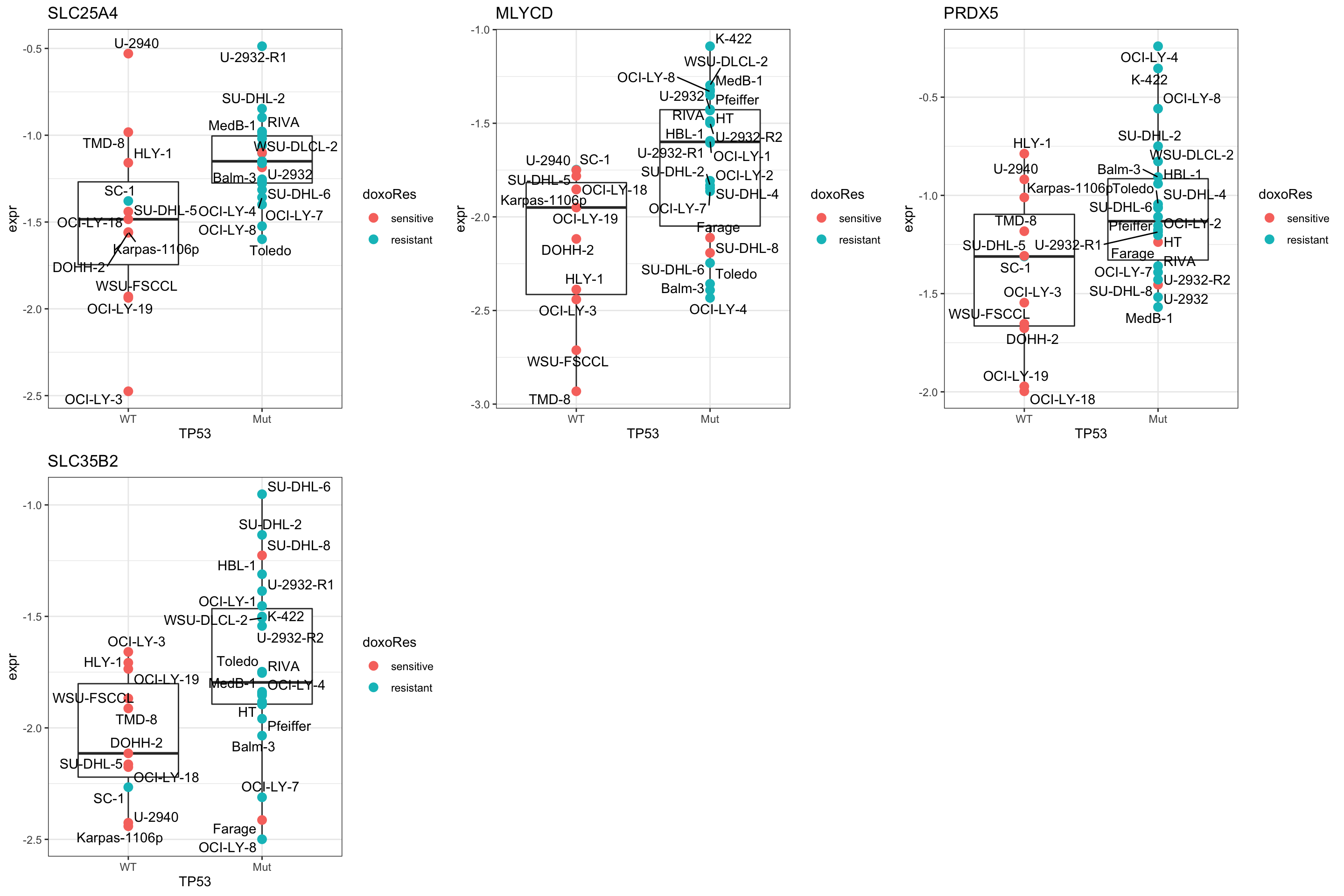
How about CPT1A?
plotGene <- filter(resTab, symbol%in% "CPT1A")
pList <- lapply(seq(nrow(plotGene)), function(i) {
  rec <- plotGene[i,]
  plotTab <- tibble(expr = protMat[rec$name,],
                    TP53 = protSub$TP53,
                    doxoRes = protSub$doxoRes,
                    Name = colnames(protMat))
  ggplot(plotTab, aes(x=TP53, y=expr)) +
    geom_boxplot(outlier.shape = NA) +
    ggbeeswarm::geom_quasirandom(aes(color = doxoRes), size=3) +
    ggrepel::geom_text_repel(aes(label = Name)) +
    ggtitle(rec$symbol) +
    theme_bw()
})

cowplot::plot_grid(plotlist = pList,ncol=1)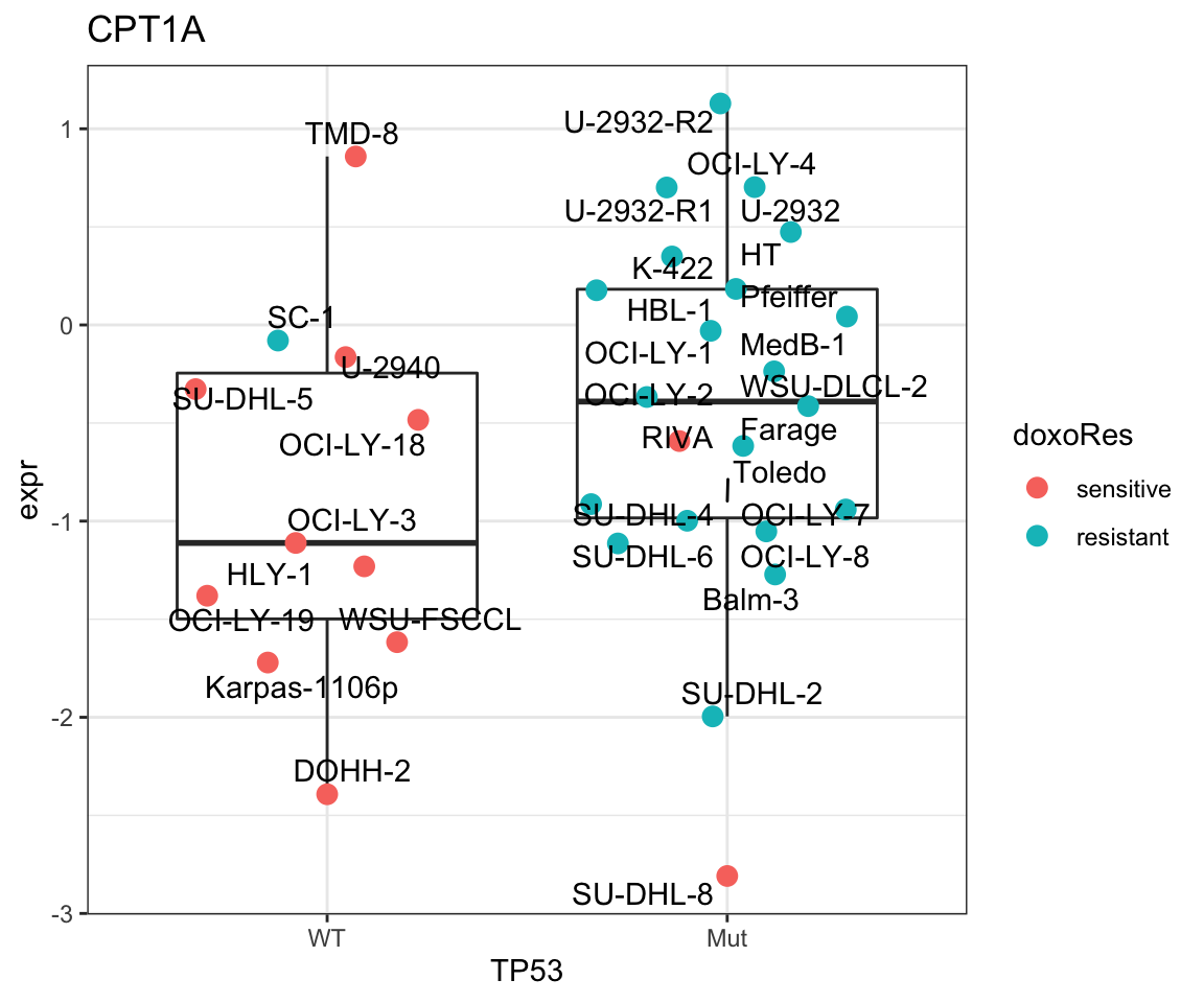
Compare the baseline results from the two datasets
resTab.com <- bind_rows(
  mutate(resTab.base.smart, set ="SMART"),
  mutate(resTab.base.embl, set = "EMBL")
) %>%
  mutate(direction = ifelse(t_statistic >0, "Up_in_resistant", "Down_in_resistant")) %>%
  select(symbol, set, direction, pval)
Plot p-values
plotTab <- resTab.com %>%
  group_by(symbol, set, direction) %>%
  summarise(pval = min(pval)) %>%
  pivot_wider(names_from = set, values_from = pval) %>%
  filter(!is.na(SMART),!is.na(EMBL)) %>%
  mutate(sig = case_when(
    EMBL <= 0.05 & SMART <= 0.05 ~ "both",
    EMBL <= 0.05 & SMART >= 0.05 ~ "only EMBL",
    EMBL >= 0.05 & SMART <= 0.05 ~ "only SMART"
  ))

#how many commonly detected proteins?
nrow(plotTab)
[1] 1717ggplot(plotTab, aes(x=-log10(SMART),y=-log10(EMBL))) +
geom_point(aes(col = sig)) +
geom_smooth(method = "lm") +
facet_wrap(~direction) +
ggrepel::geom_text_repel(data = filter(plotTab, sig == "both"), aes(label = symbol)) +
theme_bw()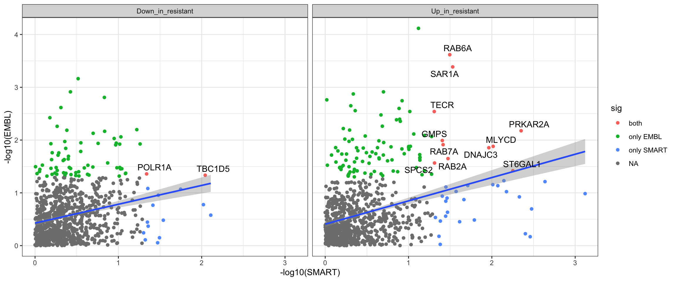
Identify proteins differentially expressed between Doxorubicine resistant and sensitive samples
Differential protein expression using proDA
protMat <- assay(protSub)
fit <- proDA(protMat, design = ~ doxoRes,
             col_data = colData(protSub))

resTab <- test_diff(fit, contrast = "doxoResresistant") %>%
  arrange(pval) %>%
  mutate(symbol = rowData(protSub[name,])$symbol)

resTab.doxo <- resTab
hist(resTab.doxo$pval)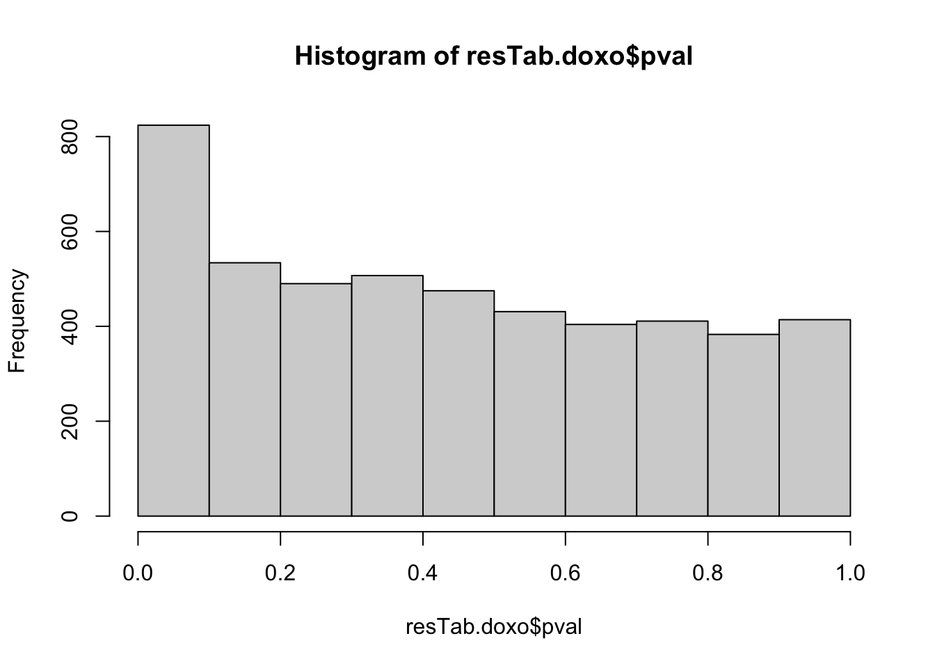 Stronger associations can be observed
Compare the p-values with TP53 related proteins. The proteins with significant p-value change are potentially the proteins that can explain why SU-DHL-8 are sensitive.
pComTab <- resTab.base.embl %>%
  select(name, pval, diff) %>%
  dplyr::rename(pval.tp53 = pval, diff.tp53 = diff) %>%
  left_join(resTab.doxo %>% select(name, pval, diff) %>%
              dplyr::rename(pval.doxo = pval, diff.doxo = diff),
            by = "name") %>%
  mutate(pDiff = -log10(pval.doxo) + log10(pval.tp53),
         fcDiff = diff.doxo -diff.tp53) %>%
  arrange(desc(pDiff))

seleTab <- filter(pComTab, pval.doxo < 0.05)
seleTab %>% mutate_if(is.numeric, formatC, digits=1) %>%
  DT::datatable()
ggplot(pComTab, aes(x=-log10(pval.tp53), y=-log10(pval.doxo))) +
geom_point() +
xlim(0,5) + ylim(0,5) +
geom_abline(intercept = 0, slope = 1, col = "red") +
ggrepel::geom_label_repel(data = filter(seleTab, pDiff > 0.8), aes(label = name), max.overlaps = Inf) +
theme_bw()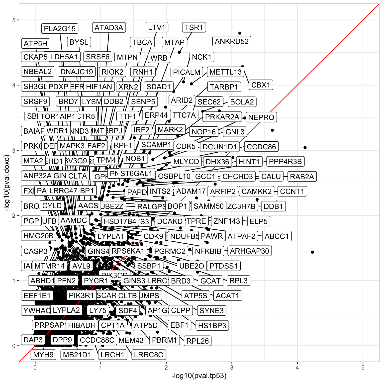
Plot top 9 examples
pList <- lapply(seq(9), function(i) {
  rec <- seleTab[i,]
  plotTab <- tibble(expr = protMat[rec$name,],
                    TP53 = protSub$TP53,
                    Name = colnames(protSub),
                    doxoRes = protSub$doxoRes)
  ggplot(plotTab, aes(x=TP53, y=expr)) +
    geom_boxplot(outlier.shape = NA) +
    geom_point(aes(color = doxoRes), size=3) +
    ggrepel::geom_text_repel(aes(label = Name)) +
    ggtitle(rec$name) +
    theme_bw()
})

cowplot::plot_grid(plotlist = pList,ncol=3)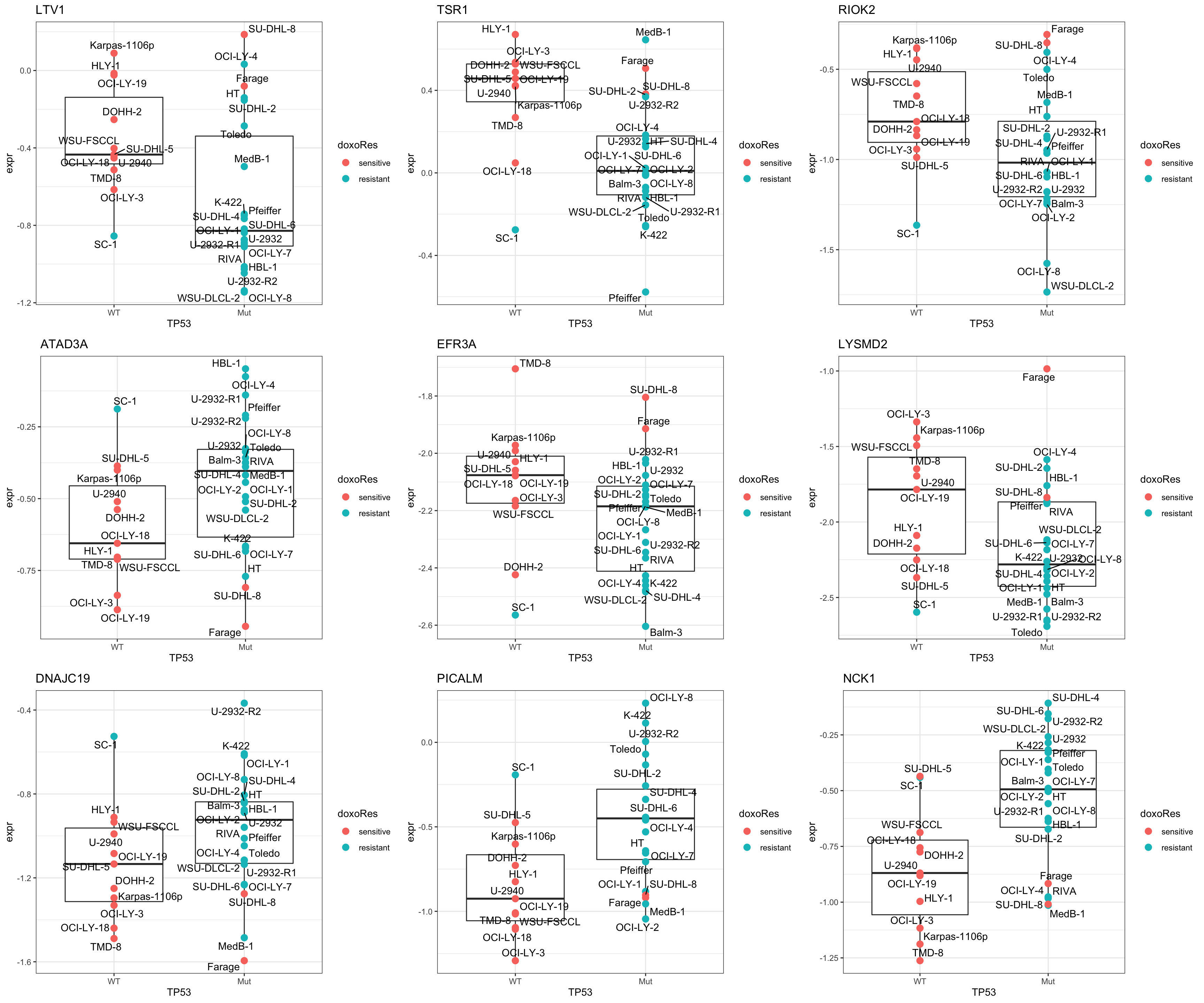
Check DLBCL cell lines with HSD17B4 mutation
filter(SVs, Gene == "HSD17B4")# A tibble: 8 × 10
Name Gene Chromos…¹ Posit…² REF ALT Class…³ Cosmi…⁴ Categ…⁵ Cosmi…⁶
<chr> <chr> <chr> <int> <chr> <chr> <chr> <chr> <chr> <chr>
1 CA-46 HSD17B4 5 1.19e8 G A nonsyn… Yes SNV Substi…
2 DG-75 HSD17B4 5 1.19e8 G A nonsyn… No SNV <NA>
3 L-1236 HSD17B4 5 1.19e8 A G synony… No SNV <NA>
4 L-1236 HSD17B4 5 1.19e8 C T synony… No SNV <NA>
5 L-82 HSD17B4 5 1.19e8 G A nonsyn… No SNV <NA>
6 MEC-1 HSD17B4 5 1.19e8 C G nonsyn… No SNV <NA>
7 MEC-2 HSD17B4 5 1.19e8 C G nonsyn… No SNV <NA>
8 SU-DHL-4 HSD17B4 5 1.19e8 C T synony… No SNV <NA>
# … with abbreviated variable names ¹Chromosome, ²Position, ³Classification,
# ⁴Cosmic_old, ⁵Category, ⁶Cosmic_newNo SU-DHL-8. Perhaps there’s a deletion?
Enrichment analysis
gmts = list(H= "../data/gmts/h.all.v6.2.symbols.gmt",
            KEGG = "../data/gmts/c2.cp.kegg.v6.2.symbols.gmt",
            C6 = "../data/gmts/c6.all.v6.2.symbols.gmt")
inputTab <- seleTab %>%
  distinct(name, .keep_all = TRUE) %>%
  select(name, fcDiff) %>% data.frame() %>% column_to_rownames("name")
enRes <- list()
enRes[["Hallmark"]] <- runGSEA(inputTab, gmts$H, "page")
enRes[["KEGG"]] <- runGSEA(inputTab, gmts$KEGG,"page")
enRes[["Perturbation"]] <- runGSEA(inputTab, gmts$C6,"page")
p <- jyluMisc::plotEnrichmentBar(enRes, pCut =0.1, ifFDR= TRUE)
cowplot::plot_grid(p)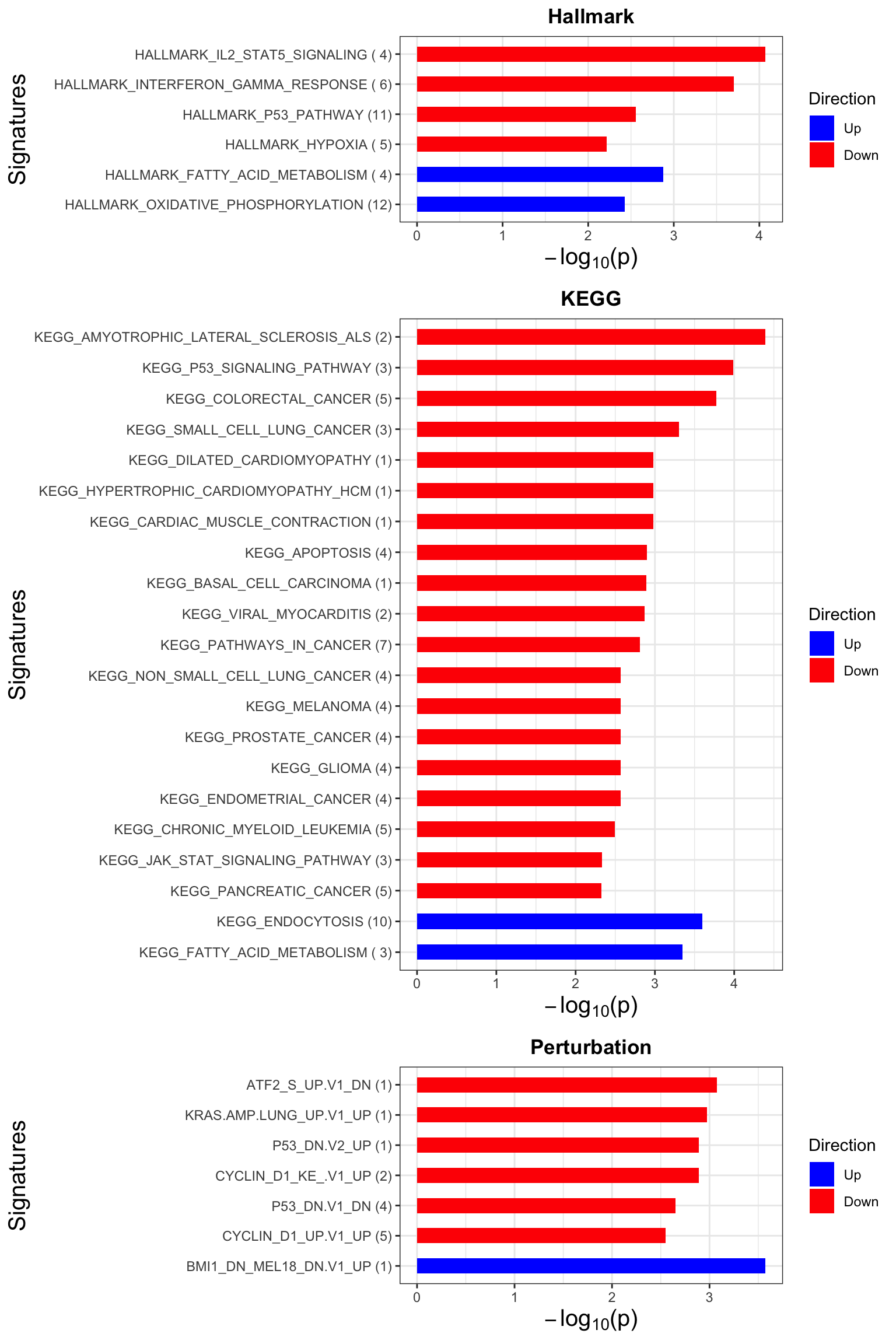
Focus on proteins from Fatty acid metabolism pathway
geneList <- piano::loadGSC(gmts$H)$gsc$HALLMARK_FATTY_ACID_METABOLISM
plotGene <- filter(seleTab, name%in% geneList )
pList <- lapply(seq(nrow(plotGene)), function(i) {
  rec <- plotGene[i,]
  plotTab <- tibble(expr = protMat[rec$name,],
                    Name = colnames(protMat),
                    TP53 = protSub$TP53,
                    doxoRes = protSub$doxoRes)
  ggplot(plotTab, aes(x=TP53, y=expr)) +
    geom_boxplot(outlier.shape = NA) +
    geom_point(aes(color = doxoRes), size=3) +
    ggrepel::geom_text_repel(aes(label = Name)) +
    ggtitle(rec$name) +
    theme_bw()
})

cowplot::plot_grid(plotlist = pList,ncol=3)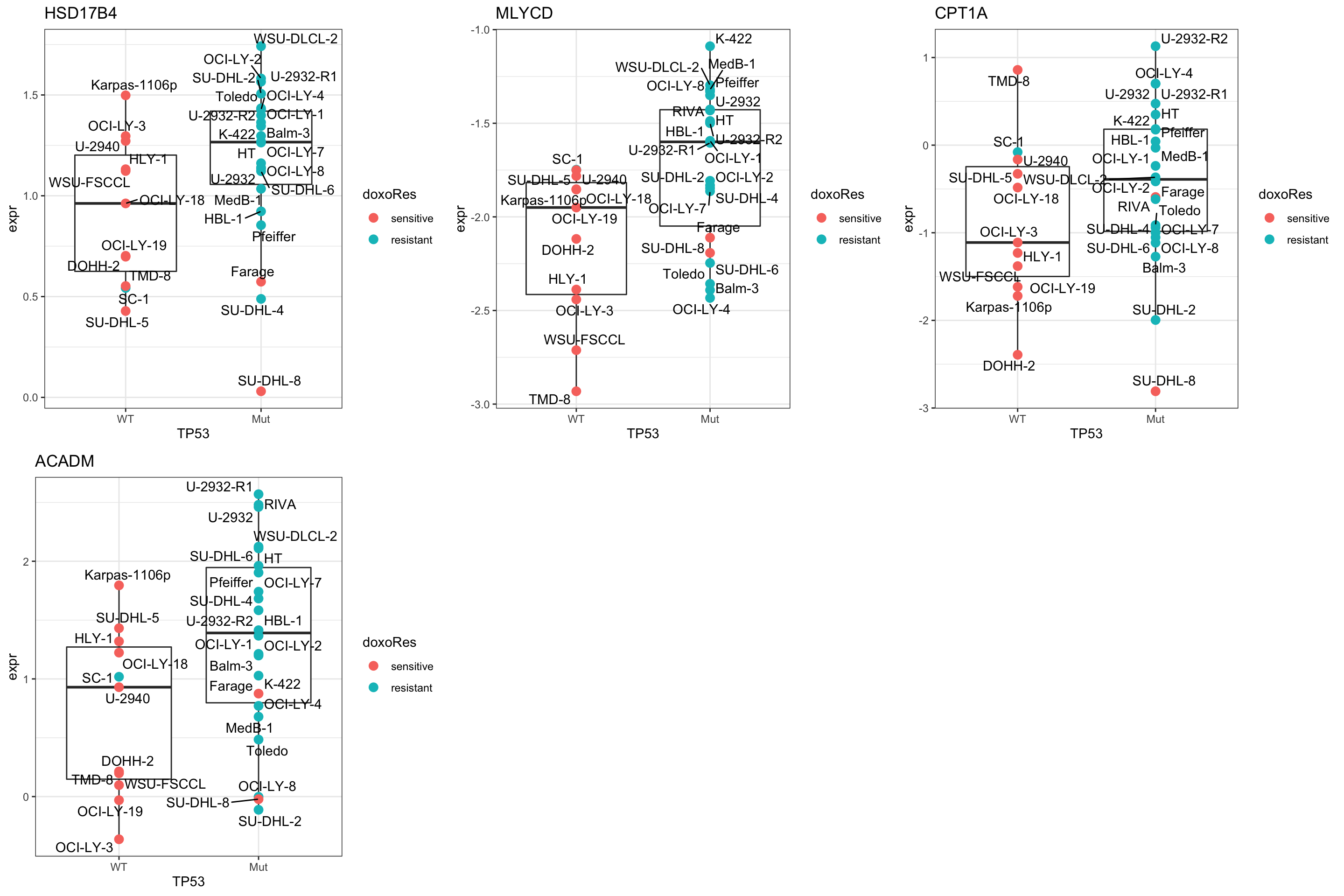
Metabolimics
The metabolic dataset does not have SU-DHL-8 cell line
Process metabolomic data
Normalization
metaData <- readRDS("../data/SC005_SummarizedExperiment_metabolomics.RDS")
metaData <- metaData[,metaData$cell.line %in% tp53MutTab$Name]
metaMat <- assay(metaData)
boxplot(metaMat)
metaMatNorm <- PhosR::medianScaling(metaMat, scale = FALSE)
#vsnFit <- vsn::vsnMatrix(metaMat)
#metaMatNorm <- metaMat
boxplot(metaMatNorm)
metaNorm <- metaData
assay(metaNorm) <- metaMatNorm
assayNames(metaNorm) <- "norm"
Average technical replicates for each cell line
metaTab <- jyluMisc::sumToTidy(metaNorm) %>%
  group_by(cell.line, rowID, metabolite, class, condition) %>%
  summarise(count = mean(norm, na.rm=TRUE)) %>%
  dplyr::rename(symbol = metabolite, cellLine = cell.line) %>%
  mutate(colID = paste0(cellLine,"_", condition)) %>%
  ungroup()
Create SE object
metaAll <- jyluMisc::tidyToSum(metaTab, rowID = "rowID", colID = "colID",
                     values = "count", annoRow = "symbol",
                     annoCol = c("condition", "cellLine"))

#add additional annotations
metaAll$doxoRes <- tp53MutTab[match(metaAll$cellLine, tp53MutTab$Name),]$doxoRes
metaAll$TP53 <- tp53MutTab[match(metaAll$cellLine, tp53MutTab$Name),]$status

#remove uncessary samples and records
metaAll <- metaAll[!rowData(metaAll)$symbol %in% c("",NA), !is.na(metaAll$TP53)]
dim(metaAll)
[1] 286 24colData(metaAll) %>% data.frame() %>% DT::datatable()No SU-DHL-8 cell line
Differential expression in Baseline (Untreated) condition
metaSub <- metaAll[,metaAll$condition == "U"]Differential metabolites abundance
metaMat <- assay(metaSub)
designMat <- model.matrix(~metaSub$TP53)
fit <- lmFit(metaMat, designMat)
fit2 <- eBayes(fit)

resTab <- topTable(fit2, number= Inf) %>%
  dplyr::rename(pval = P.Value, adj_pval = adj.P.Val) %>%
  arrange(pval) %>%
  as_tibble(rownames = "name") %>%
  mutate(symbol = rowData(metaSub[name,])$symbol)
hist(resTab$pval)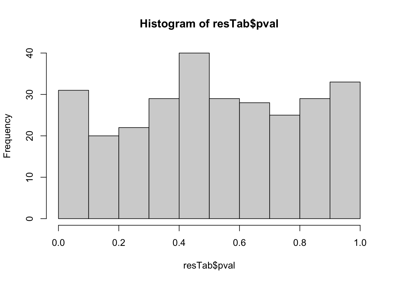 Not strong difference
Show all metabolites
resTab.sig <- filter(resTab)
resTab.sig %>% select(symbol, pval, adj_pval, logFC, t) %>%
  mutate_if(is.numeric, formatC, digits=1) %>%
  DT::datatable()
Plot top 9 examples
pList <- lapply(seq(9), function(i) {
  rec <- resTab.sig[i,]
  plotTab <- tibble(expr = metaMat[rec$name,],
                    TP53 = metaSub$TP53,
                    Name = colnames(metaSub))
  ggplot(plotTab, aes(x=TP53, y=expr)) +
    geom_boxplot(outlier.shape = NA) +
    geom_point(aes(color = TP53), size=3) +
    ggrepel::geom_text_repel(aes(label = Name)) +
    ggtitle(rec$symbol) +
    theme_bw() +
    theme(legend.position = "none")
})

cowplot::plot_grid(plotlist = pList,ncol=3)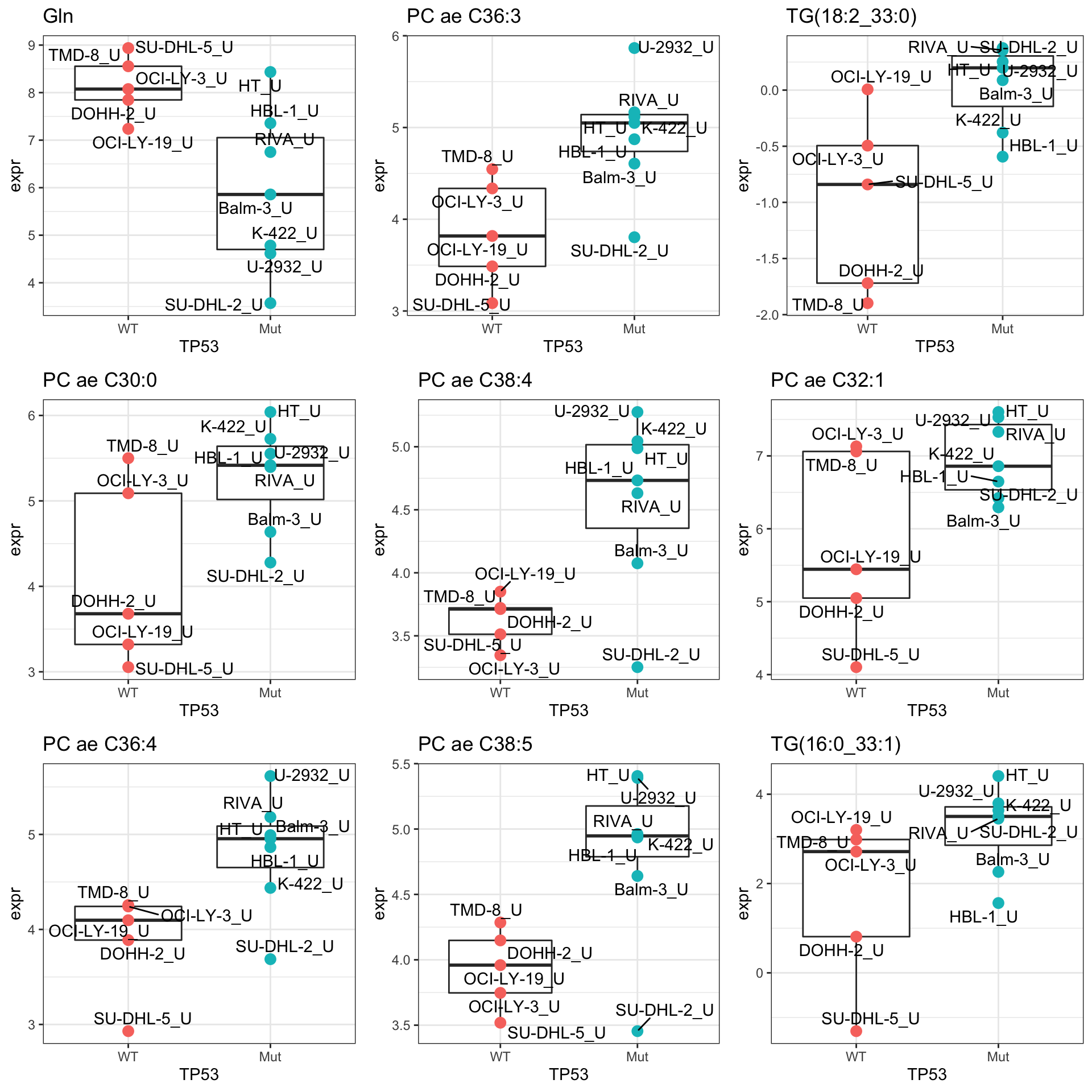
Differential expression before and after treatment
metaSub <- metaAllDifferential metabolites abundance
metaMat <- assay(metaSub)
designMat <- model.matrix(~cellLine + condition, colData(metaSub))
fit <- lmFit(metaMat, designMat)
fit2 <- eBayes(fit)

resTab <- topTable(fit2, number= Inf, coef = "conditionT") %>%
  dplyr::rename(pval = P.Value, adj_pval = adj.P.Val) %>%
  arrange(pval) %>%
  as_tibble(rownames = "name") %>%
  mutate(symbol = rowData(metaSub[name,])$symbol)
hist(resTab$pval)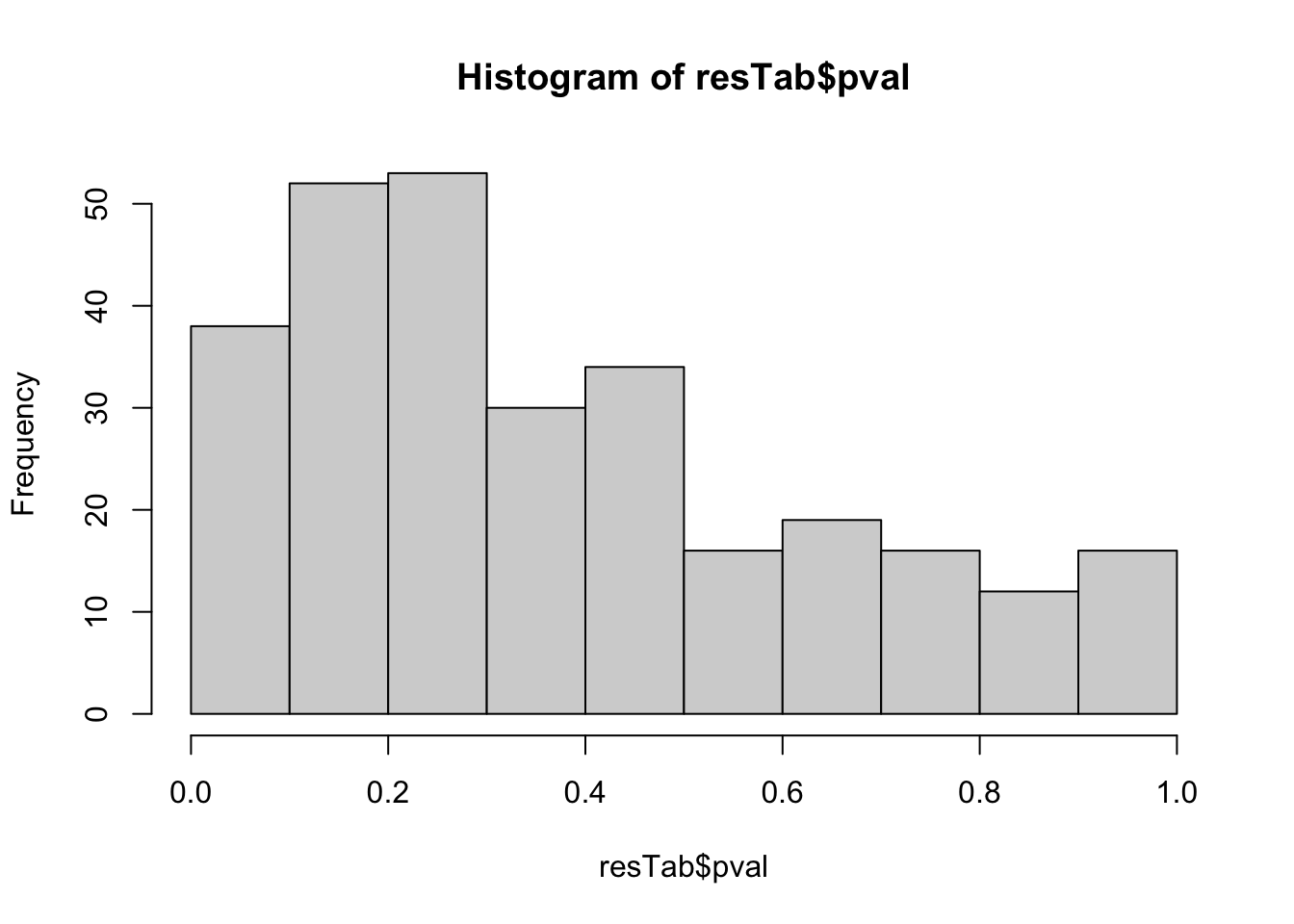 Some difference can be detected
Proteins with p-value < 0.05
resTab.sig <- filter(resTab, pval < 0.05)
resTab.sig %>% select(symbol, pval, adj_pval, logFC, t) %>%
  mutate_if(is.numeric, formatC, digits=1) %>%
  DT::datatable()
Plot top 9 examples
pList <- lapply(seq(9), function(i) {
  rec <- resTab.sig[i,]
  plotTab <- tibble(expr = metaMat[rec$name,],
                    TP53 = metaSub$TP53,
                    Name = metaSub$cellLine,
                    condition = metaSub$condition)
  ggplot(plotTab, aes(x=condition, y=expr)) +
    geom_boxplot(outlier.shape = NA) +
    geom_point(aes(color = TP53), size=3) +
    geom_line(aes(group = Name), linetype = "dotted") +
    ggrepel::geom_text_repel(aes(label = Name)) +
    ggtitle(rec$symbol) +
    theme_bw()
})

cowplot::plot_grid(plotlist = pList,ncol=3)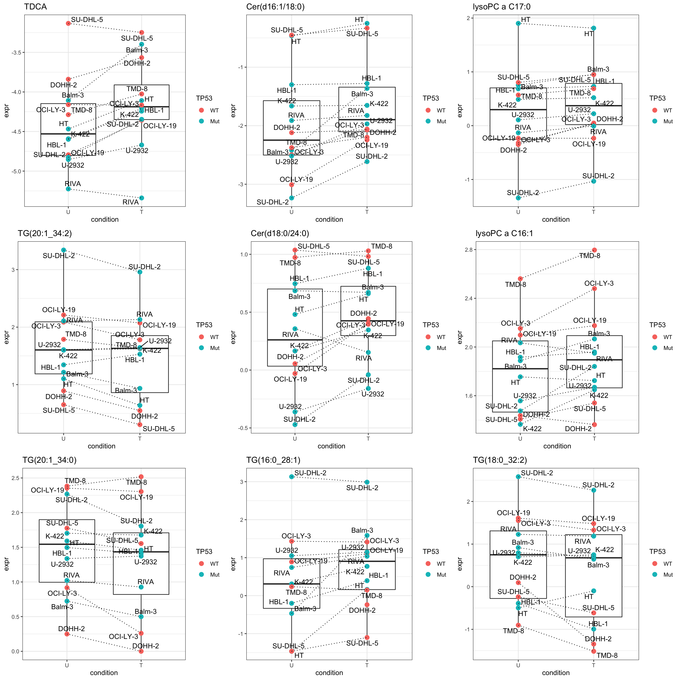
Interaction between treatment and sensitivity cluster
metaSub <- metaAllDifferential protein expression using proDA
metaMat <- assay(metaSub)
design <- model.matrix(~ 0 + condition*TP53, data = colData(metaSub))
colnames(design) <- make.names(colnames(design))

cor <- duplicateCorrelation(metaMat, design, block=metaSub$cellLine)
#cor$consensus.correlation

fit <- lmFit(object=metaMat, design=design, block=metaSub$cellLine,
    correlation = cor$consensus.correlation, method = "ls")
fit2 <- eBayes(fit)
resTab  <- topTable(fit2, number = Inf, coef="conditionT.TP53Mut") %>%
  as_tibble(rownames = "name") %>%
  mutate(symbol = rowData(metaSub[name,])$symbol) %>%
  dplyr::rename(pval = P.Value, adj_pval = adj.P.Val, diff = logFC, t_statistics = t)
hist(resTab$pval)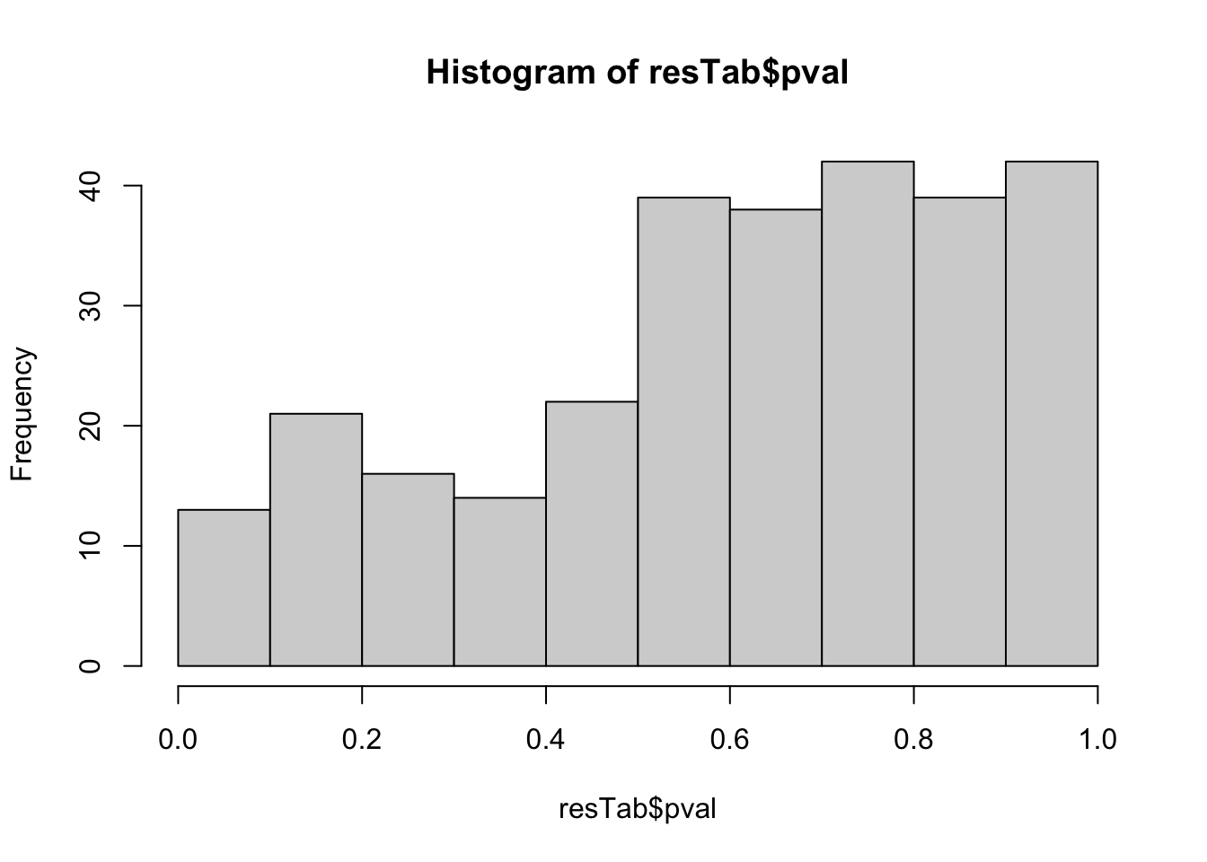 Not strong difference
Proteins with p-value < 0.05
resTab.sig <- filter(resTab, pval < 0.05)
resTab.sig %>% select(symbol, pval, adj_pval, diff) %>%
  mutate_if(is.numeric, formatC, digits=1) %>%
  DT::datatable()
Plot top 9 examples
pList <- lapply(seq(9), function(i) {
  rec <- resTab.sig[i,]
  plotTab <- tibble(expr = metaMat[rec$name,],
                    TP53 = metaSub$TP53,
                    Name = metaSub$cellLine,
                    condition = metaSub$condition)
  ggplot(plotTab, aes(x=condition, y=expr)) +
    geom_boxplot(outlier.shape = NA) +
    geom_point(aes(color = TP53), size=3) +
    geom_line(aes(group = Name), linetype = "dotted") +
    ggrepel::geom_text_repel(aes(label = Name)) +
    ggtitle(rec$symbol) +
    theme_bw() +
    facet_wrap(~TP53)
})

cowplot::plot_grid(plotlist = pList,ncol=3)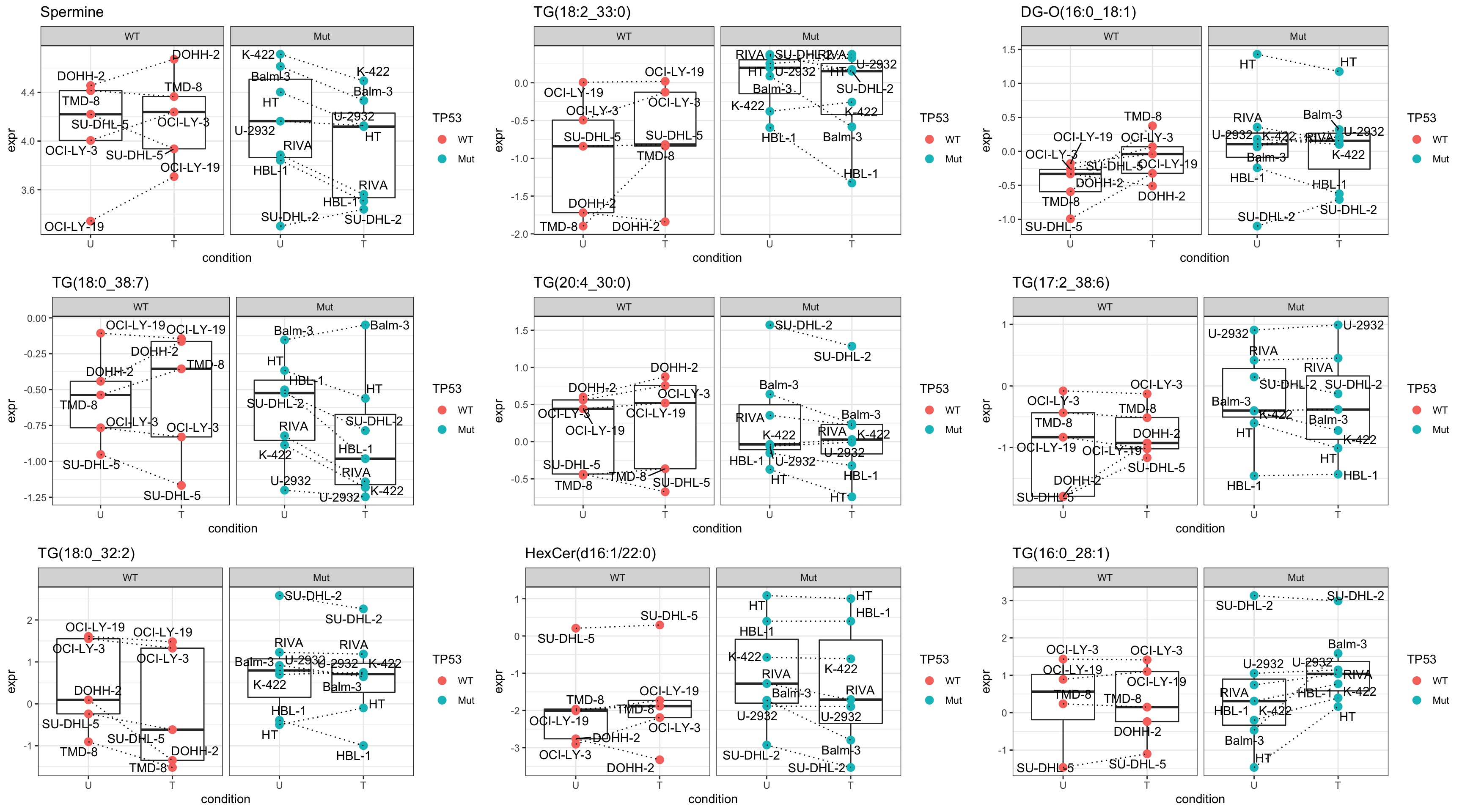
Metabolimics (average lipids from the same classes)
Process metabolomic data
Normalization
metaData <- readRDS("../data/SC005_SummarizedExperiment_metabolomics.RDS")
metaData <- metaData[,metaData$cell.line %in% tp53MutTab$Name]
metaMat <- assay(metaData)
boxplot(metaMat)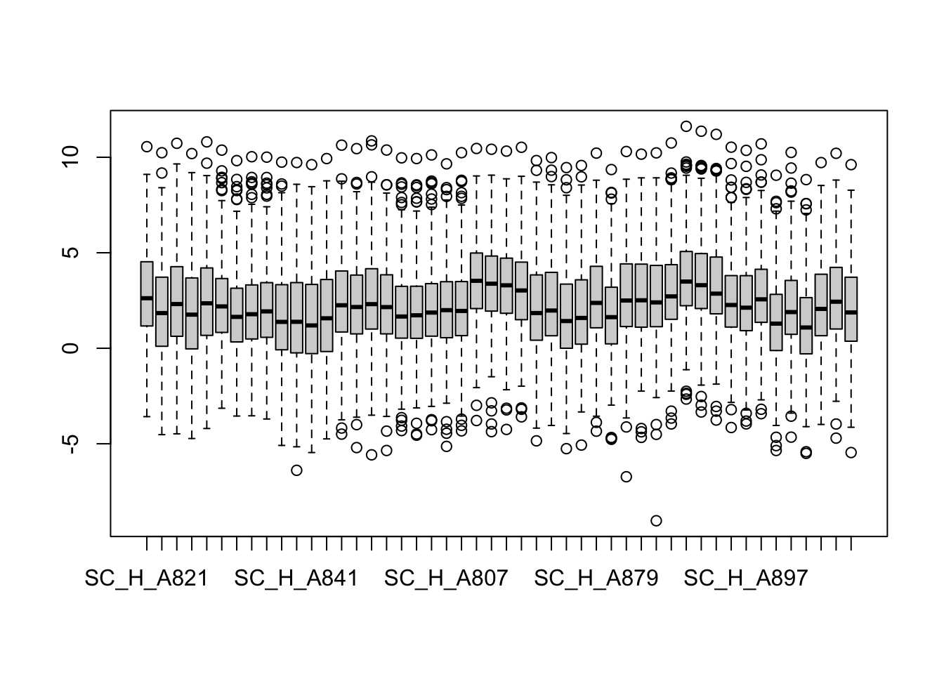
metaMatNorm <- PhosR::medianScaling(metaMat, scale = FALSE)
#vsnFit <- vsn::vsnMatrix(metaMat)
#metaMatNorm <- metaMat
boxplot(metaMatNorm)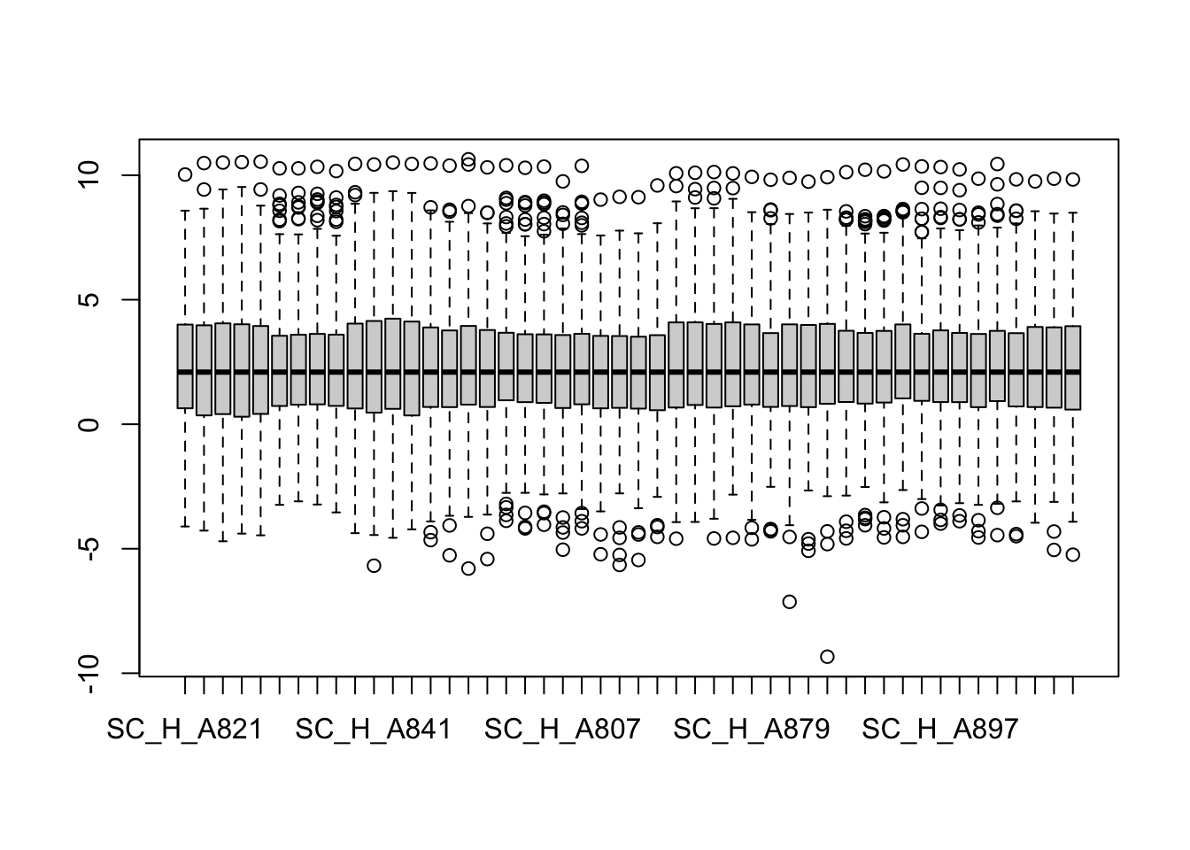
metaNorm <- metaData
assay(metaNorm) <- metaMatNorm
assayNames(metaNorm) <- "norm"
Average technical replicates for each cell line
metaTab <- jyluMisc::sumToTidy(metaNorm) %>%
  group_by(cell.line, rowID, metabolite, class, condition) %>%
  summarise(count = mean(norm, na.rm=TRUE)) %>%
  dplyr::rename(symbol = metabolite, cellLine = cell.line) %>%
  mutate(colID = paste0(cellLine,"_", condition)) %>%
  ungroup()
Number of species per class
spTab <- metaTab %>% distinct(class, symbol) %>%
  group_by(class) %>% summarise(num = length(symbol)) %>%
  arrange(desc(num))
spTab %>% DT::datatable()
Average lipid classes
metaTab <- group_by(metaTab, cellLine, class, condition, colID) %>%
  summarise(count= mean(count)) %>%
  ungroup() %>% mutate(symbol = class, rowID = class)
Create SE object
metaAll <- jyluMisc::tidyToSum(metaTab, rowID = "rowID", colID = "colID",
                     values = "count", annoRow = "symbol",
                     annoCol = c("condition", "cellLine"))

#add additional annotations
metaAll$doxoRes <- tp53MutTab[match(metaAll$cellLine, tp53MutTab$Name),]$doxoRes
metaAll$TP53 <- tp53MutTab[match(metaAll$cellLine, tp53MutTab$Name),]$status

#remove uncessary samples and records
metaAll <- metaAll[!rowData(metaAll)$symbol %in% c("",NA), !is.na(metaAll$TP53)]
dim(metaAll)
[1] 17 24Differential expression in Baseline (Untreated) condition
metaSub <- metaAll[,metaAll$condition == "U"]Differential metabolites abundance
metaMat <- assay(metaSub)
designMat <- model.matrix(~metaSub$TP53)
fit <- lmFit(metaMat, designMat)
fit2 <- eBayes(fit)

resTab <- topTable(fit2, number= Inf) %>%
  dplyr::rename(pval = P.Value, adj_pval = adj.P.Val) %>%
  arrange(pval) %>%
  as_tibble(rownames = "name") %>%
  mutate(symbol = rowData(metaSub[name,])$symbol)
hist(resTab$pval)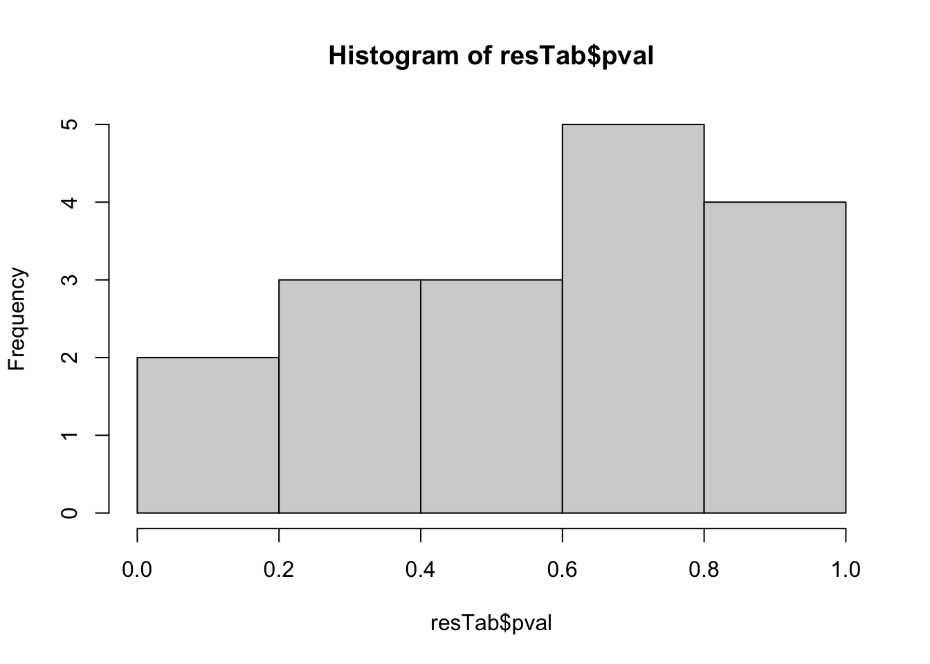 Not strong difference
Show all metabolites
resTab.sig <- filter(resTab)
resTab.sig %>% select(symbol, pval, adj_pval, logFC, t) %>%
  mutate_if(is.numeric, formatC, digits=1) %>%
  DT::datatable()
Plot top 9 examples
pList <- lapply(seq(9), function(i) {
  rec <- resTab.sig[i,]
  plotTab <- tibble(expr = metaMat[rec$name,],
                    TP53 = metaSub$TP53,
                    Name = colnames(metaSub))
  ggplot(plotTab, aes(x=TP53, y=expr)) +
    geom_boxplot(outlier.shape = NA) +
    geom_point(aes(color = TP53), size=3) +
    ggrepel::geom_text_repel(aes(label = Name)) +
    ggtitle(rec$symbol) +
    theme_bw() +
    theme(legend.position = "none")
})

cowplot::plot_grid(plotlist = pList,ncol=3)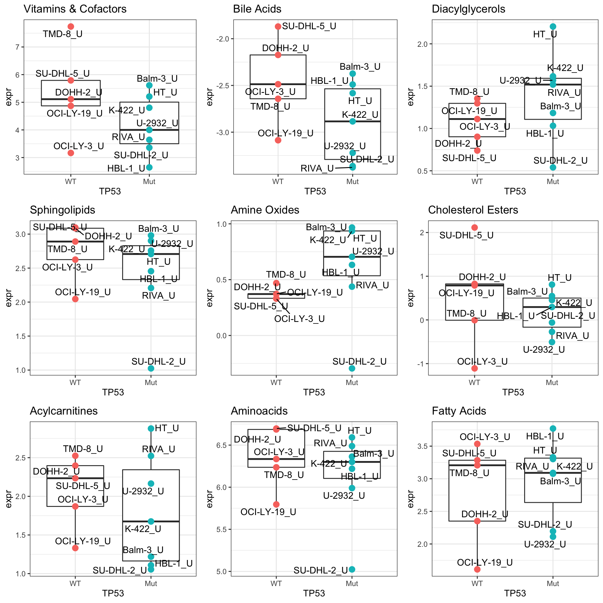
Differential expression before and after treatment
metaSub <- metaAllDifferential metabolites abundance
metaMat <- assay(metaSub)
designMat <- model.matrix(~cellLine + condition, colData(metaSub))
fit <- lmFit(metaMat, designMat)
fit2 <- eBayes(fit)

resTab <- topTable(fit2, number= Inf, coef = "conditionT") %>%
  dplyr::rename(pval = P.Value, adj_pval = adj.P.Val) %>%
  arrange(pval) %>%
  as_tibble(rownames = "name") %>%
  mutate(symbol = rowData(metaSub[name,])$symbol)
hist(resTab$pval)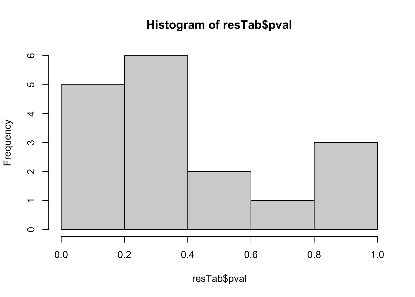 Some difference can be detected
Proteins with p-value < 0.05
resTab.sig <- filter(resTab, pval < 0.05)
resTab.sig %>% select(symbol, pval, adj_pval, logFC, t) %>%
  mutate_if(is.numeric, formatC, digits=1) %>%
  DT::datatable()
Plot top 9 examples
pList <- lapply(seq(9), function(i) {
  rec <- resTab[i,]
  plotTab <- tibble(expr = metaMat[rec$name,],
                    TP53 = metaSub$TP53,
                    Name = metaSub$cellLine,
                    condition = metaSub$condition)
  ggplot(plotTab, aes(x=condition, y=expr)) +
    geom_boxplot(outlier.shape = NA) +
    geom_point(aes(color = TP53), size=3) +
    geom_line(aes(group = Name), linetype = "dotted") +
    ggrepel::geom_text_repel(aes(label = Name)) +
    ggtitle(rec$symbol) +
    theme_bw()
})

cowplot::plot_grid(plotlist = pList,ncol=3)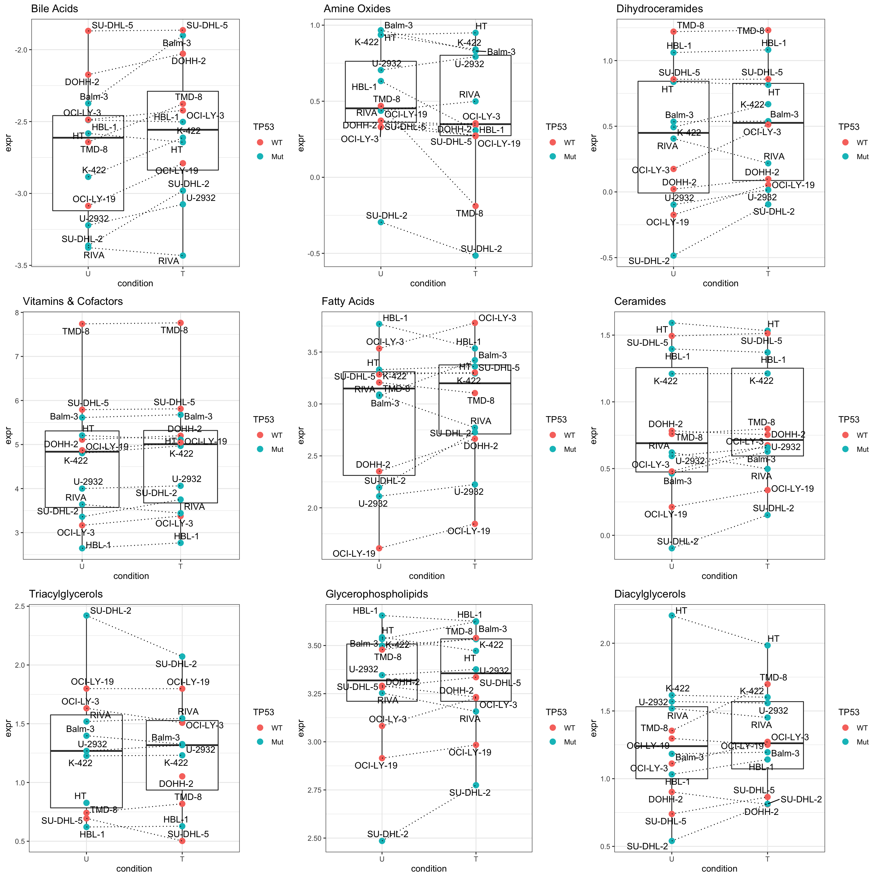
Interaction between treatment and sensitivity cluster
metaSub <- metaAllDifferential protein expression using proDA
metaMat <- assay(metaSub)
design <- model.matrix(~ 0 + condition*TP53, data = colData(metaSub))
colnames(design) <- make.names(colnames(design))

cor <- duplicateCorrelation(metaMat, design, block=metaSub$cellLine)
#cor$consensus.correlation

fit <- lmFit(object=metaMat, design=design, block=metaSub$cellLine,
    correlation = cor$consensus.correlation, method = "ls")
fit2 <- eBayes(fit)
resTab  <- topTable(fit2, number = Inf, coef="conditionT.TP53Mut") %>%
  as_tibble(rownames = "name") %>%
  mutate(symbol = rowData(metaSub[name,])$symbol) %>%
  dplyr::rename(pval = P.Value, adj_pval = adj.P.Val, diff = logFC, t_statistics = t)
hist(resTab$pval)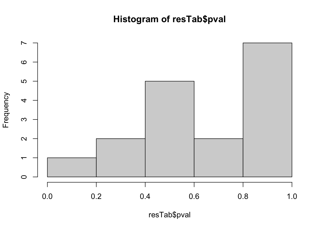 Not strong difference
Proteins with p-value < 0.05
resTab.sig <- filter(resTab, pval < 0.05)
resTab.sig %>% select(symbol, pval, adj_pval, diff) %>%
  mutate_if(is.numeric, formatC, digits=1) %>%
  DT::datatable()
Differential gene expression analysis based on public data
Proprocessing
load("../data/DepMap_GEXwide.RData")
exprMat <- t(DepMap_GEXwide)
exprMat <- exprMat[,colnames(exprMat) %in% tp53MutTab$Name]

# Remove low count genes
exprMat <- exprMat[rowMedians(exprMat) >0,]

dim(exprMat)
[1] 15422 15boxplot(exprMat)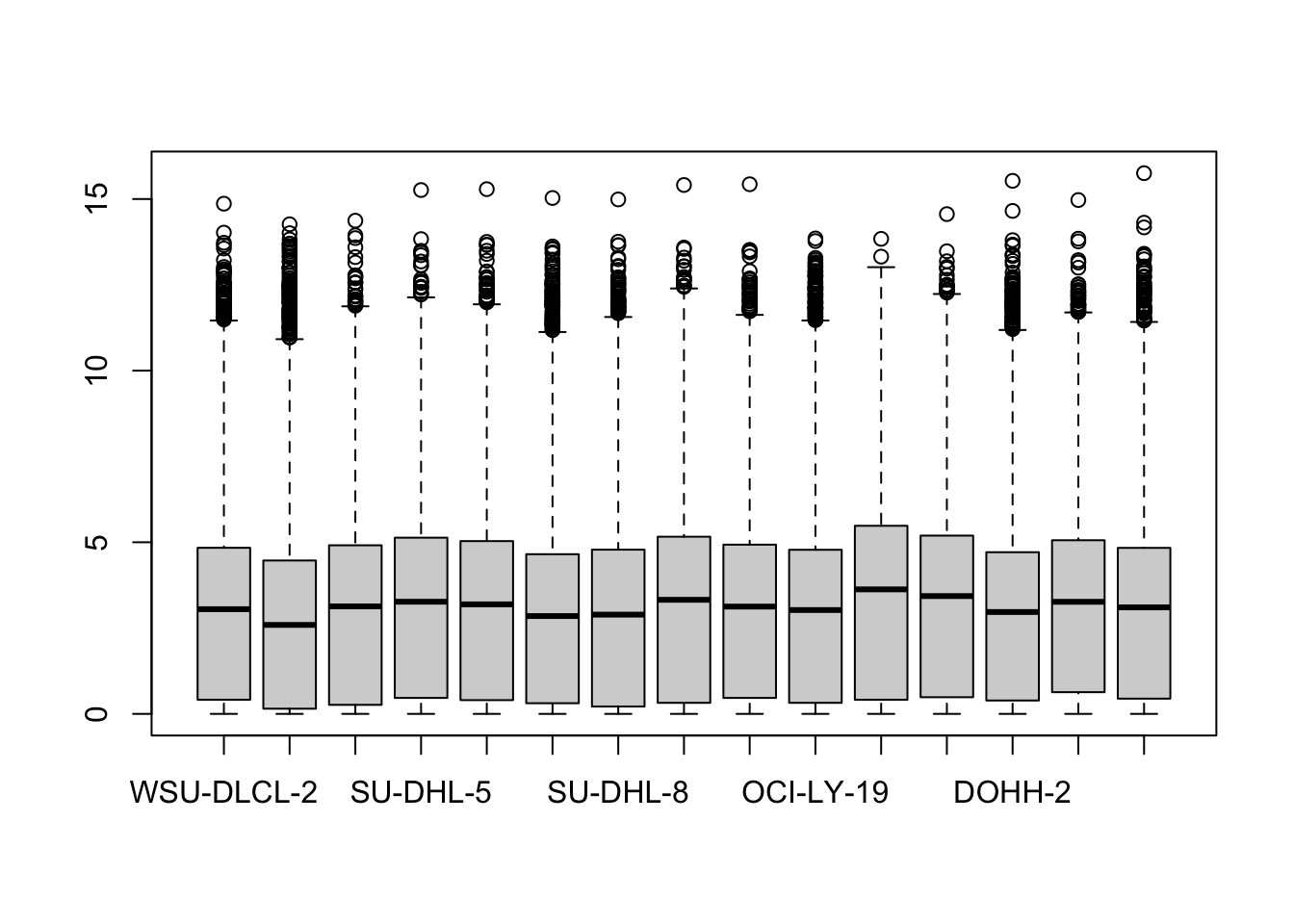
vstObj <- vsn::vsnMatrix(exprMat)
exprMat <- vsn::predict(vstObj, exprMat)

boxplot(exprMat)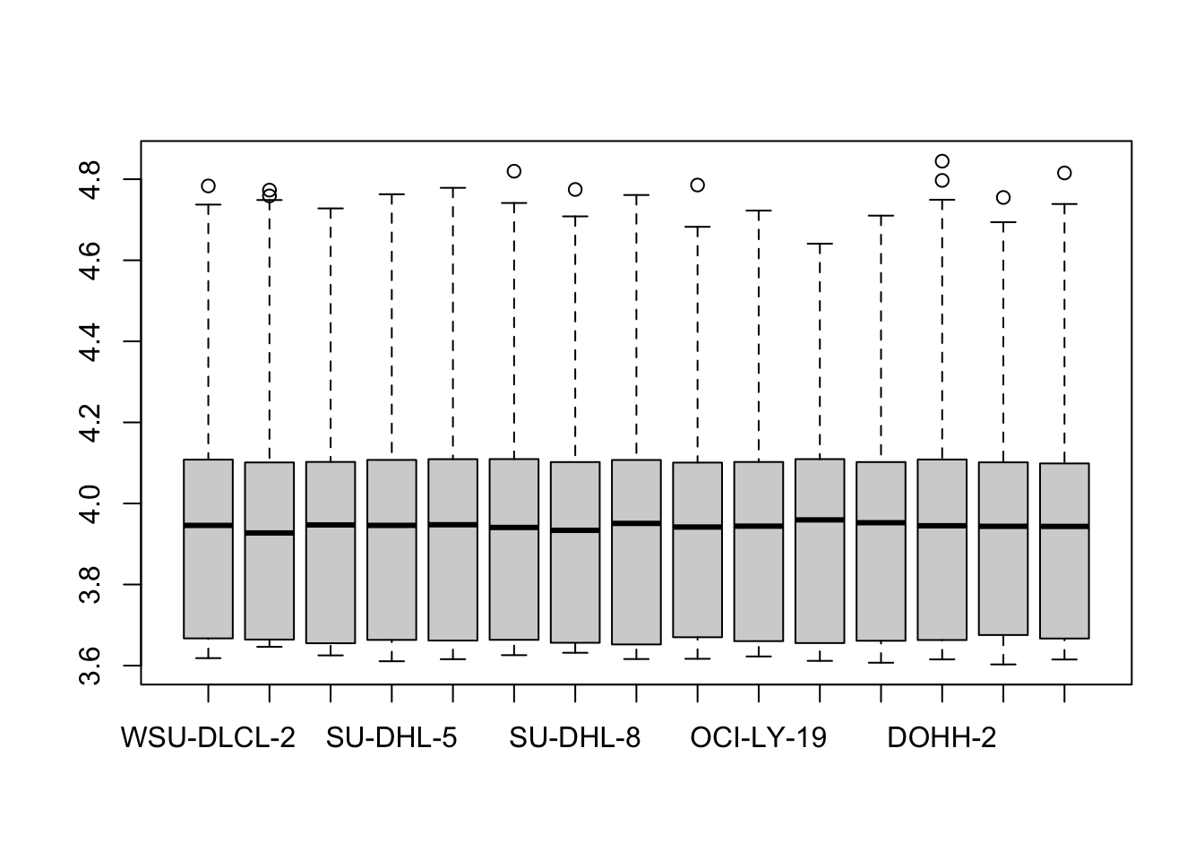
#save process data
#save(exprMat, file = "gene_exprMat.RData")
colnames(exprMat) [1] "WSU-DLCL-2" "Farage" "OCI-LY-7" "SU-DHL-5" "SU-DHL-6"
[6] "SU-DHL-4" "SU-DHL-8" "HT" "RIVA" "OCI-LY-19"
[11] "K-422" "Toledo" "DOHH-2" "Pfeiffer" "OCI-LY-3" SU-DHL-8 is in the dataset
Differential expression using limma
colTab <- tp53MutTab[match(colnames(exprMat), tp53MutTab$Name),] %>%
  column_to_rownames("Name") %>% data.frame()
designMat <- model.matrix(~status, colTab)

fit <- lmFit(exprMat, designMat)
fit2 <- eBayes(fit)
resTab <- topTable(fit2, number = Inf) %>%
  as_tibble(rownames = "symbol")
Associations with p <= 0.05
resTab.sig <- filter(resTab, P.Value <= 0.05)
resTab.sig %>% mutate_if(is.numeric, formatC, digits=2) %>% DT::datatable()
Plot top 9 examples
pList <- lapply(seq(9), function(i) {
  rec <- resTab.sig[i,]
  plotTab <- tibble(expr = exprMat[rec$symbol,],
                    TP53 = colTab$status,
                    doxoRes = colTab$doxoRes,
                    Name = colnames(exprMat))
  ggplot(plotTab, aes(x=TP53, y=expr)) +
    geom_boxplot(outlier.shape = NA) +
    geom_point(aes(color = doxoRes), size=3) +
    ggrepel::geom_text_repel(aes(label = Name)) +
    ggtitle(rec$symbol) +
    theme_bw() +
    theme(legend.position = "none")
})

cowplot::plot_grid(plotlist = pList,ncol=3)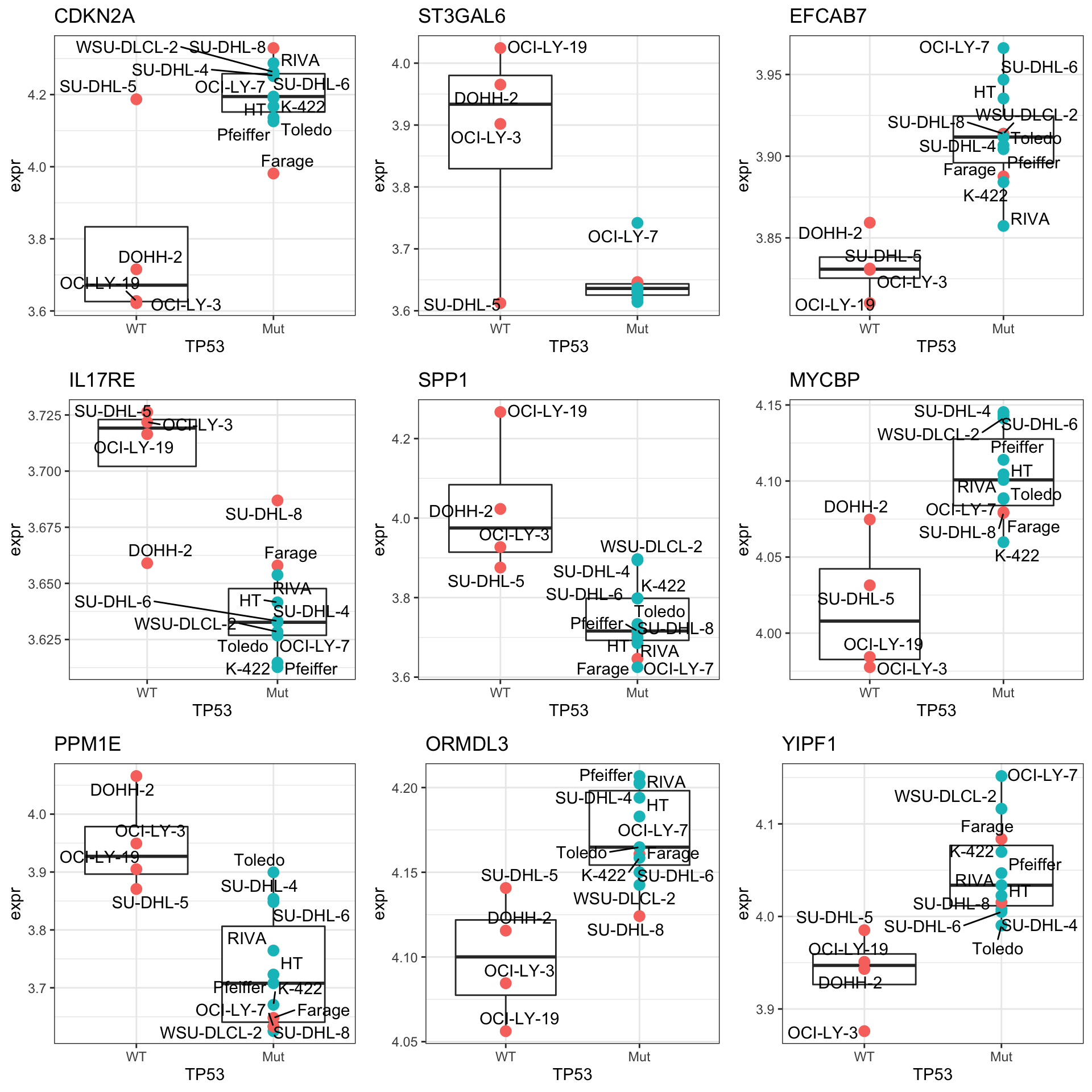
Enrichment analysis
gmts = list(H= "../data/gmts/h.all.v6.2.symbols.gmt",
            KEGG = "../data/gmts/c2.cp.kegg.v6.2.symbols.gmt",
            C6 = "../data/gmts/c6.all.v6.2.symbols.gmt")
inputTab <- resTab %>% filter(P.Value < 0.05) %>%
  distinct(symbol, .keep_all = TRUE) %>%
  select(symbol, t) %>% data.frame() %>% column_to_rownames("symbol")
enRes <- list()
enRes[["Hallmark"]] <- runGSEA(inputTab, gmts$H, "page")
enRes[["KEGG"]] <- runGSEA(inputTab, gmts$KEGG,"page")
enRes[["Perturbation"]] <- runGSEA(inputTab, gmts$C6,"page")
p <- jyluMisc::plotEnrichmentBar(enRes, pCut =0.1, ifFDR= TRUE)
cowplot::plot_grid(p)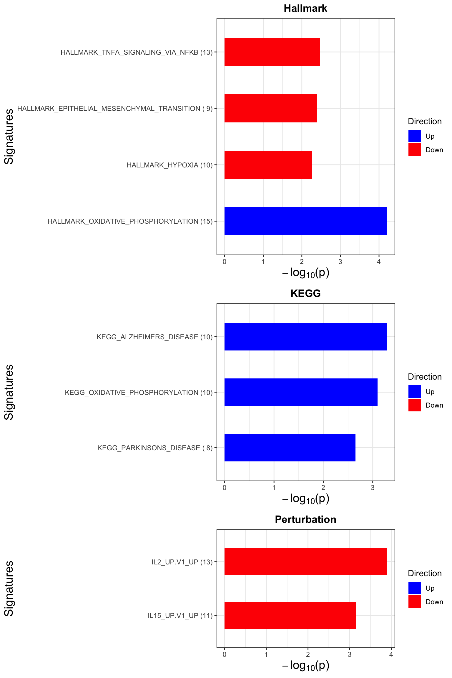
Focus on proteins from Fatty acid metabolism pathway
geneList <- piano::loadGSC(gmts$H)$gsc$HALLMARK_FATTY_ACID_METABOLISM
plotGene <- filter(filter(resTab, P.Value <= 0.05), symbol%in% geneList )
pList <- lapply(seq(nrow(plotGene)), function(i) {
  rec <- plotGene[i,]
  plotTab <- tibble(expr = exprMat[rec$symbol,],
                    TP53 = colTab$status,
                    doxoRes = colTab$doxoRes,
                    Name = colnames(exprMat))
  ggplot(plotTab, aes(x=TP53, y=expr)) +
    geom_boxplot(outlier.shape = NA) +
    geom_point(aes(color = doxoRes), size=3) +
    ggrepel::geom_text_repel(aes(label = Name), max.overlaps = Inf) +
    ggtitle(rec$symbol) +
    theme_bw() +
    theme(legend.position = "none")
})

cowplot::plot_grid(plotlist = pList,ncol=3)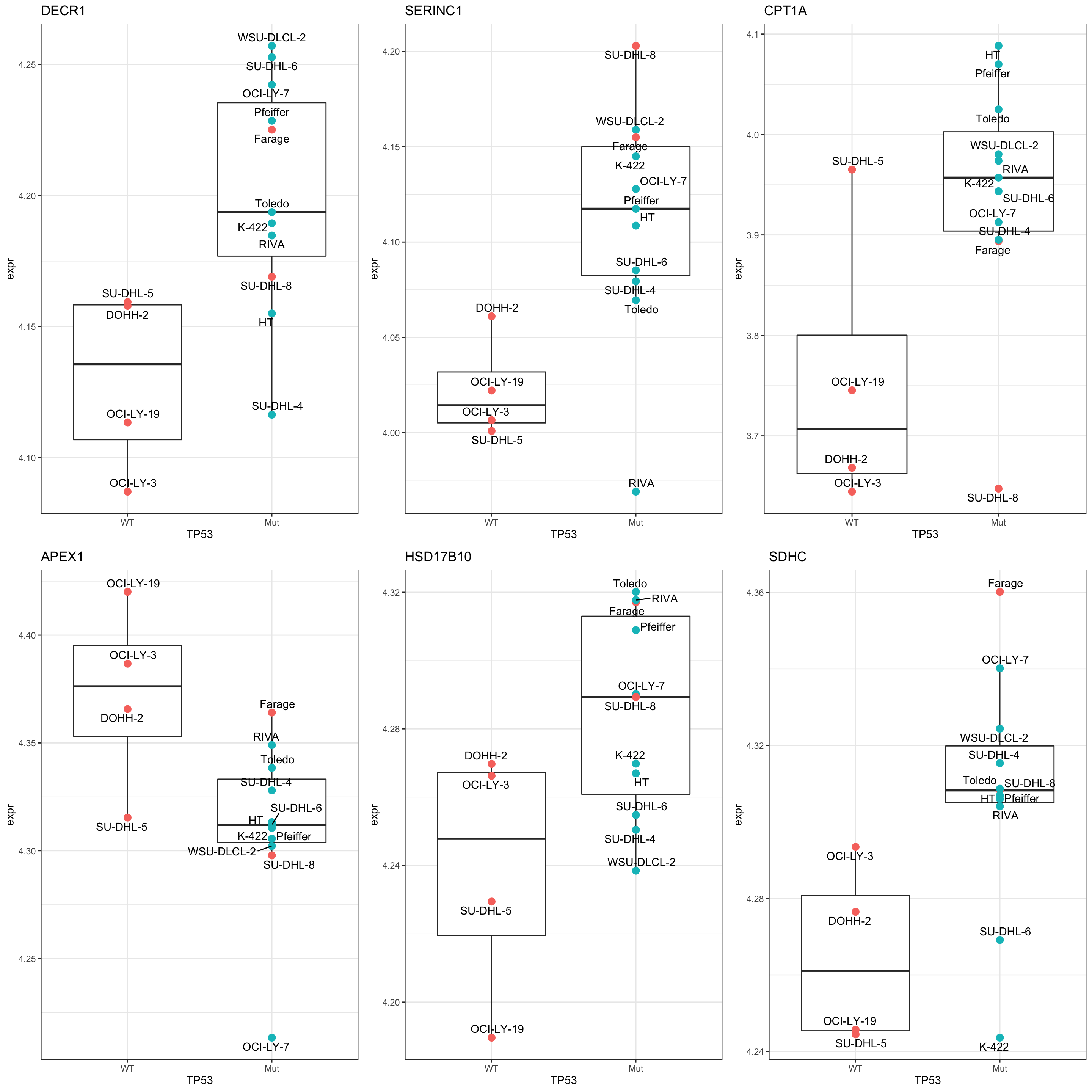
Compare TP53 mutation signature and Doxo response signature
DE test
colTab <- tp53MutTab[match(colnames(exprMat), tp53MutTab$Name),] %>%
  column_to_rownames("Name") %>% data.frame()
designMat <- model.matrix(~doxoRes, colTab)

fit <- lmFit(exprMat, designMat)
fit2 <- eBayes(fit)
resTab.doxo <- topTable(fit2, number = Inf) %>%
  as_tibble(rownames = "symbol")
hist(resTab.doxo$P.Value)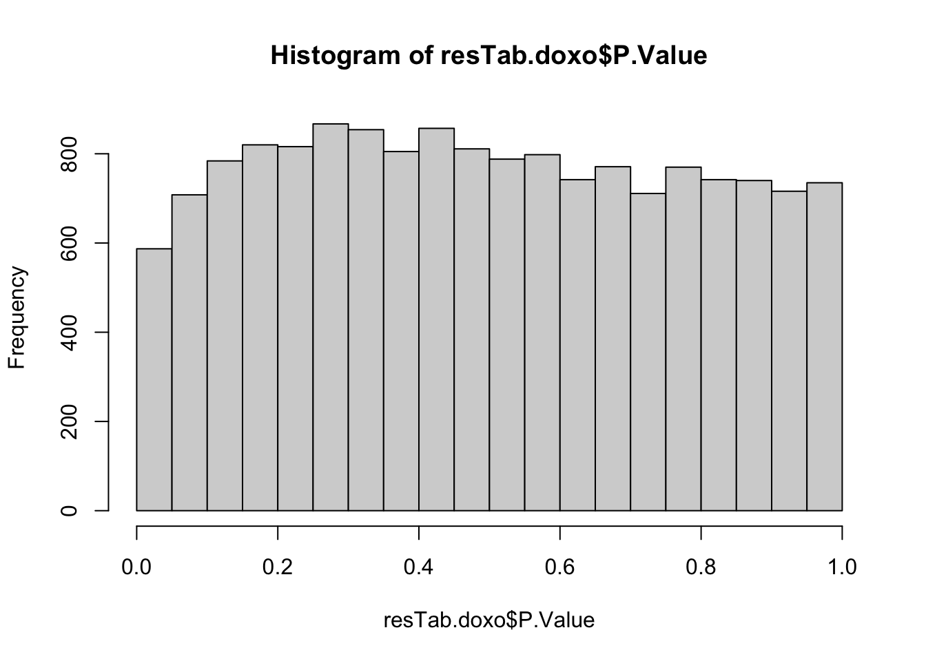
Compare the p-values with TP53 related gene The gene with significant p-value change are potentially the proteins that can explain why SU-DHL-8 are sensitive.
pComTab <- resTab %>%
  select(symbol, P.Value, logFC) %>%
  dplyr::rename(pval.tp53 = P.Value, diff.tp53 = logFC) %>%
  left_join(resTab.doxo %>% select(symbol, P.Value, logFC) %>%
              dplyr::rename(pval.doxo = P.Value, diff.doxo = logFC),
            by = "symbol") %>%
  mutate(pDiff = -log10(pval.doxo) + log10(pval.tp53),
         fcDiff = diff.doxo - diff.tp53) %>%
  arrange(desc(pDiff))

seleTab <- filter(pComTab, pval.doxo < 0.05)
seleTab %>% mutate_if(is.numeric, formatC, digits=1) %>%
  DT::datatable()
ggplot(pComTab, aes(x=-log10(pval.tp53), y=-log10(pval.doxo))) +
geom_point() +
xlim(0,5) + ylim(0,5) +
geom_abline(intercept = 0, slope = 1, col = "red") +
ggrepel::geom_label_repel(data = filter(seleTab, pDiff >1), aes(label = symbol), max.overlaps = Inf) +
theme_bw()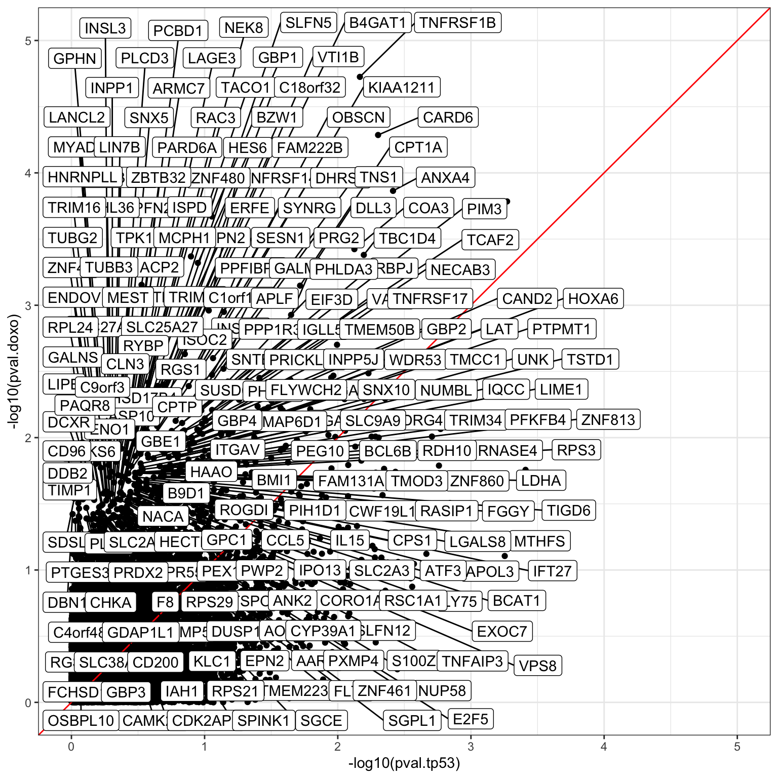
Plot top 9 examples
pList <- lapply(seq(9), function(i) {
  rec <- seleTab[i,]
  plotTab <- tibble(expr = exprMat[rec$symbol,],
                    TP53 = colTab$status,
                    doxoRes = colTab$doxoRes,
                    Name = colnames(exprMat))
  ggplot(plotTab, aes(x=TP53, y=expr)) +
    geom_boxplot(outlier.shape = NA) +
    geom_point(aes(color = doxoRes), size=3) +
    ggrepel::geom_text_repel(aes(label = Name)) +
    ggtitle(rec$symbol) +
    theme_bw()
})

cowplot::plot_grid(plotlist = pList,ncol=3)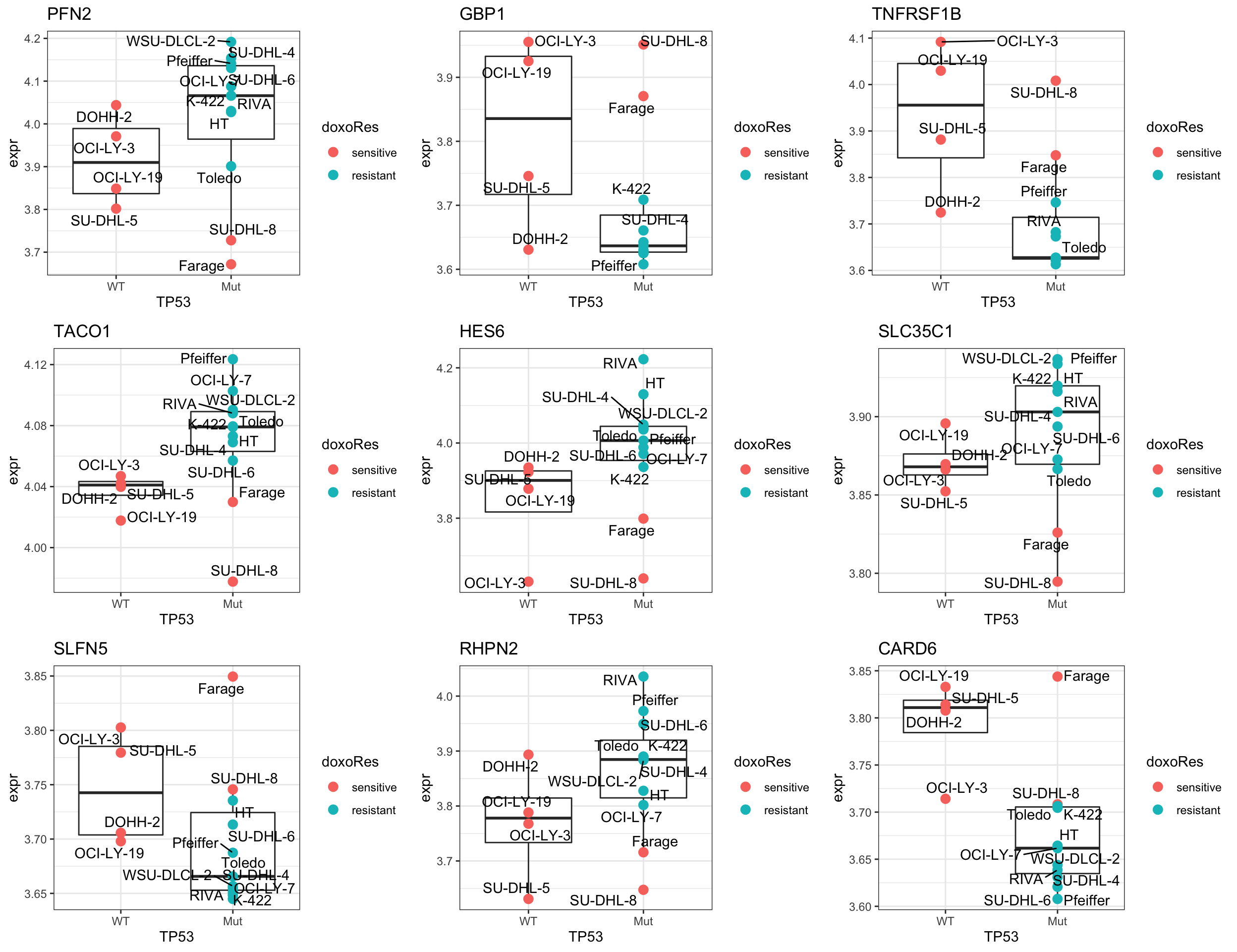
Plot HSD17B4
plotTab <- tibble(expr = exprMat["HSD17B4",],
                  TP53 = colTab$status,
                  doxoRes = colTab$doxoRes,
                  Name = colnames(exprMat))
ggplot(plotTab, aes(x=TP53, y=expr)) +
  geom_boxplot(outlier.shape = NA) +
  geom_point(aes(color = doxoRes), size=3) +
  ggrepel::geom_text_repel(aes(label = Name)) +
  ggtitle("HSD17B4") +
theme_bw() 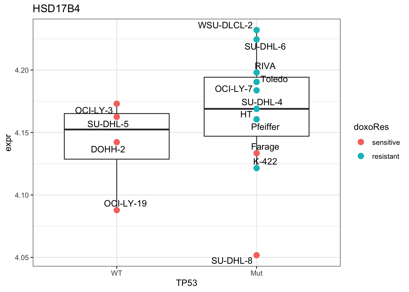
Plot CPT1A
plotTab <- tibble(expr = exprMat["CPT1A",],
                  TP53 = colTab$status,
                  doxoRes = colTab$doxoRes,
                  Name = colnames(exprMat))
ggplot(plotTab, aes(x=TP53, y=expr)) +
  geom_boxplot(outlier.shape = NA) +
  geom_point(aes(color = doxoRes), size=3) +
  ggrepel::geom_text_repel(aes(label = Name)) +
  ggtitle("CPT1A") +
theme_bw() 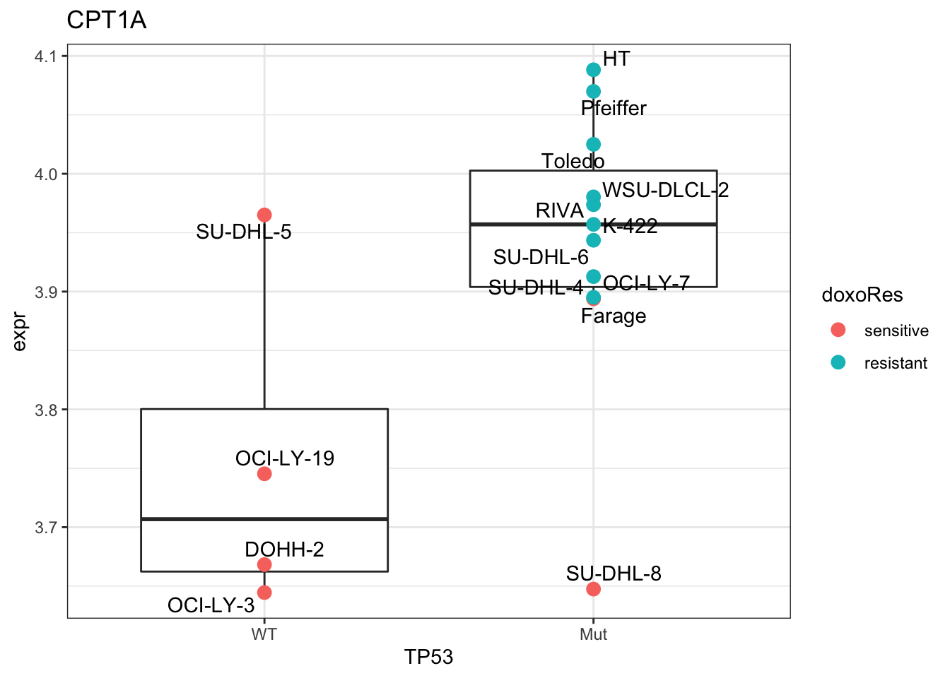
Enrichment analysis
gmts = list(H= "../data/gmts/h.all.v6.2.symbols.gmt",
            KEGG = "../data/gmts/c2.cp.kegg.v6.2.symbols.gmt",
            C6 = "../data/gmts/c6.all.v6.2.symbols.gmt")
inputTab <- seleTab %>%
  distinct(symbol, .keep_all = TRUE) %>%
  select(symbol, fcDiff) %>% data.frame() %>% column_to_rownames("symbol")
enRes <- list()
enRes[["Hallmark"]] <- runGSEA(inputTab, gmts$H, "page")
enRes[["KEGG"]] <- runGSEA(inputTab, gmts$KEGG,"page")
enRes[["Perturbation"]] <- runGSEA(inputTab, gmts$C6,"page")
p <- jyluMisc::plotEnrichmentBar(enRes, pCut =0.1, ifFDR= TRUE)
[1] "No sets passed the criteria"cowplot::plot_grid(p)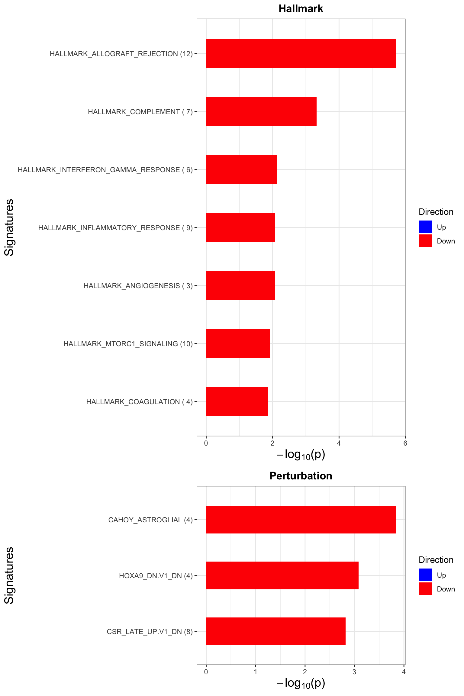 Focus on genes from Fatty acid metabolism pathway
geneList <- piano::loadGSC(gmts$H)$gsc$HALLMARK_FATTY_ACID_METABOLISM
plotGene <- filter(seleTab, symbol%in% geneList )
pList <- lapply(seq(nrow(plotGene)), function(i) {
  rec <- plotGene[i,]
  plotTab <- tibble(expr = exprMat[rec$symbol,],
                    TP53 = colTab$status,
                    doxoRes = colTab$doxoRes,
                    Name = colnames(exprMat))
  ggplot(plotTab, aes(x=TP53, y=expr)) +
    geom_boxplot(outlier.shape = NA) +
    geom_point(aes(color = doxoRes), size=3) +
    ggrepel::geom_text_repel(aes(label = Name), max.overlaps = Inf) +
    ggtitle(rec$symbol) +
    theme_bw()
})

cowplot::plot_grid(plotlist = pList,ncol=3)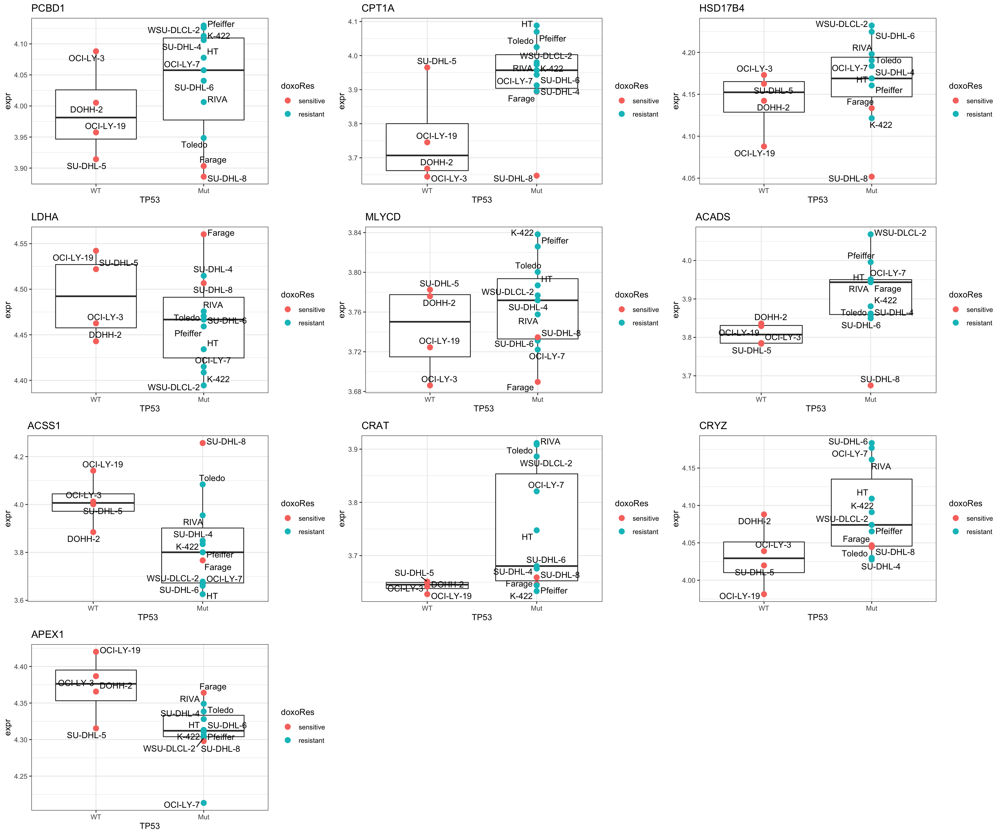
sessionInfo()R version 4.2.0 (2022-04-22)
Platform: x86_64-apple-darwin17.0 (64-bit)
Running under: macOS Big Sur/Monterey 10.16
Matrix products: default
BLAS: /Library/Frameworks/R.framework/Versions/4.2/Resources/lib/libRblas.0.dylib
LAPACK: /Library/Frameworks/R.framework/Versions/4.2/Resources/lib/libRlapack.dylib
locale:
[1] en_US.UTF-8/en_US.UTF-8/en_US.UTF-8/C/en_US.UTF-8/en_US.UTF-8
attached base packages:
[1] stats4 stats graphics grDevices utils datasets methods
[8] base
other attached packages:
[1] piano_2.12.0 forcats_0.5.1
[3] stringr_1.4.0 dplyr_1.0.9
[5] purrr_0.3.4 readr_2.1.2
[7] tidyr_1.2.0 tibble_3.1.8
[9] ggplot2_3.3.6 tidyverse_1.3.2
[11] proDA_1.10.0 cowplot_1.1.1
[13] DESeq2_1.36.0 SummarizedExperiment_1.26.1
[15] Biobase_2.56.0 GenomicRanges_1.48.0
[17] GenomeInfoDb_1.32.2 IRanges_2.30.0
[19] S4Vectors_0.34.0 BiocGenerics_0.42.0
[21] MatrixGenerics_1.8.1 matrixStats_0.62.0
[23] limma_3.52.2 jyluMisc_0.1.5
loaded via a namespace (and not attached):
[1] utf8_1.2.2 shinydashboard_0.7.2 tidyselect_1.1.2
[4] RSQLite_2.2.15 AnnotationDbi_1.58.0 htmlwidgets_1.5.4
[7] grid_4.2.0 BiocParallel_1.30.3 maxstat_0.7-25
[10] munsell_0.5.0 preprocessCore_1.58.0 codetools_0.2-18
[13] statmod_1.4.36 DT_0.23 withr_2.5.0
[16] colorspace_2.0-3 highr_0.9 knitr_1.39
[19] rstudioapi_0.13 ggsignif_0.6.3 labeling_0.4.2
[22] git2r_0.30.1 slam_0.1-50 GenomeInfoDbData_1.2.8
[25] KMsurv_0.1-5 pheatmap_1.0.12 bit64_4.0.5
[28] farver_2.1.1 rprojroot_2.0.3 coda_0.19-4
[31] vctrs_0.4.1 generics_0.1.3 TH.data_1.1-1
[34] xfun_0.31 sets_1.0-21 R6_2.5.1
[37] ggbeeswarm_0.6.0 locfit_1.5-9.6 reshape_0.8.9
[40] bitops_1.0-7 cachem_1.0.6 fgsea_1.22.0
[43] DelayedArray_0.22.0 assertthat_0.2.1 promises_1.2.0.1
[46] scales_1.2.0 multcomp_1.4-19 googlesheets4_1.0.0
[49] beeswarm_0.4.0 gtable_0.3.0 extraDistr_1.9.1
[52] affy_1.74.0 sandwich_3.0-2 workflowr_1.7.0
[55] rlang_1.0.4 genefilter_1.78.0 GlobalOptions_0.1.2
[58] splines_4.2.0 rstatix_0.7.0 gargle_1.2.0
[61] broom_1.0.0 BiocManager_1.30.18 reshape2_1.4.4
[64] yaml_2.3.5 abind_1.4-5 modelr_0.1.8
[67] crosstalk_1.2.0 backports_1.4.1 httpuv_1.6.5
[70] tools_4.2.0 relations_0.6-12 statnet.common_4.6.0
[73] affyio_1.66.0 ellipsis_0.3.2 gplots_3.1.3
[76] jquerylib_0.1.4 RColorBrewer_1.1-3 ggdendro_0.1.23
[79] proxy_0.4-27 plyr_1.8.7 Rcpp_1.0.9
[82] visNetwork_2.1.0 zlibbioc_1.42.0 RCurl_1.98-1.7
[85] ggpubr_0.4.0 viridis_0.6.2 zoo_1.8-10
[88] haven_2.5.0 ggrepel_0.9.1 cluster_2.1.3
[91] exactRankTests_0.8-35 fs_1.5.2 magrittr_2.0.3
[94] data.table_1.14.2 PhosR_1.6.0 circlize_0.4.15
[97] reprex_2.0.1 survminer_0.4.9 pcaMethods_1.88.0
[100] googledrive_2.0.0 mvtnorm_1.1-3 hms_1.1.1
[103] shinyjs_2.1.0 mime_0.12 evaluate_0.15
[106] xtable_1.8-4 XML_3.99-0.10 readxl_1.4.0
[109] shape_1.4.6 gridExtra_2.3 compiler_4.2.0
[112] KernSmooth_2.23-20 crayon_1.5.1 htmltools_0.5.3
[115] mgcv_1.8-40 later_1.3.0 tzdb_0.3.0
[118] geneplotter_1.74.0 lubridate_1.8.0 DBI_1.1.3
[121] dbplyr_2.2.1 MASS_7.3-58 Matrix_1.4-1
[124] car_3.1-0 cli_3.3.0 vsn_3.64.0
[127] marray_1.74.0 parallel_4.2.0 igraph_1.3.4
[130] pkgconfig_2.0.3 km.ci_0.5-6 xml2_1.3.3
[133] annotate_1.74.0 vipor_0.4.5 bslib_0.4.0
[136] ruv_0.9.7.1 XVector_0.36.0 drc_3.0-1
[139] rvest_1.0.2 digest_0.6.29 Biostrings_2.64.0
[142] rmarkdown_2.14 cellranger_1.1.0 fastmatch_1.1-3
[145] survMisc_0.5.6 dendextend_1.16.0 shiny_1.7.2
[148] gtools_3.9.3 lifecycle_1.0.1 nlme_3.1-158
[151] jsonlite_1.8.0 network_1.17.2 carData_3.0-5
[154] viridisLite_0.4.0 fansi_1.0.3 pillar_1.8.0
[157] GGally_2.1.2 lattice_0.20-45 KEGGREST_1.36.3
[160] fastmap_1.1.0 httr_1.4.3 plotrix_3.8-2
[163] survival_3.3-1 glue_1.6.2 png_0.1-7
[166] bit_4.0.4 class_7.3-20 stringi_1.7.8
[169] sass_0.4.2 blob_1.2.3 caTools_1.18.2
[172] memoise_2.0.1 e1071_1.7-11