Analysis of combinatorial effect between CHP and Pola
Junyan Lu
2022-04-25
Last updated: 2022-04-28
Checks: 5 1
Knit directory: combiDLBCL/analysis/
This reproducible R Markdown analysis was created with workflowr (version 1.7.0). The Checks tab describes the reproducibility checks that were applied when the results were created. The Past versions tab lists the development history.
Great job! The global environment was empty. Objects defined in the global environment can affect the analysis in your R Markdown file in unknown ways. For reproduciblity it’s best to always run the code in an empty environment.
The command set.seed(20220425) was run prior to running the code in the R Markdown file. Setting a seed ensures that any results that rely on randomness, e.g. subsampling or permutations, are reproducible.
Great job! Recording the operating system, R version, and package versions is critical for reproducibility.
Nice! There were no cached chunks for this analysis, so you can be confident that you successfully produced the results during this run.
Great job! Using relative paths to the files within your workflowr project makes it easier to run your code on other machines.
Tracking code development and connecting the code version to the results is critical for reproducibility. To start using Git, open the Terminal and type git init in your project directory.
This project is not being versioned with Git. To obtain the full reproducibility benefits of using workflowr, please see ?wflow_start.
Load libraries and datasets
Preprocessing
Get base drug only data
screenSub <- filter(screenData, Drug_A == "DMSO", Drug_B.Conc !=0)Get the effect of CHP single agent, Pola single agent and CHP+Pola
comTab <- filter(screenSub, Drug_B == "CHP_Pola") %>%
  select(Name, Drug_B, normVal, Drug_B.ConcStep) %>%
  dplyr::rename(viabObs = normVal) %>%
  mutate(Drug_A = "CHP", Drug_B = "Polatuzumab",
         Drug_A.ConcStep = Drug_B.ConcStep)

drugATab <- filter(screenSub, Drug_B == "CHP") %>%
  select(Name, Drug_B, normVal, Drug_B.ConcStep, Drug_B.Conc) %>%
  dplyr::rename(viabA = normVal) %>%
  dplyr::rename(Drug_A = Drug_B, Drug_A.ConcStep = Drug_B.ConcStep,
                Drug_A.Conc = Drug_B.Conc)

drugBTab <- filter(screenSub, Drug_B == "Polatuzumab") %>%
  select(Name, Drug_B, Drug_B.Conc, normVal, Drug_B.ConcStep, Drug_B.Conc) %>%
  dplyr::rename(viabB = normVal)
Calculate CI for the combination of CHP and Pola
synTab <- comTab %>% left_join(drugATab, by =c("Name","Drug_A","Drug_A.ConcStep")) %>%
  left_join(drugBTab, by = c("Name","Drug_B","Drug_B.ConcStep")) %>%
  mutate(viabExp = viabA*viabB) %>%
  mutate(CI = viabObs-viabExp,
         logCI = log10(viabObs/viabExp))
Visualize CI for cell line and concentration
orders <- hcOrder(synTab$Name, synTab$Drug_B.ConcStep, synTab$CI)
plotTab <- synTab %>% mutate(Name = factor(Name, levels = orders$row))
ggplot(plotTab, aes(x=Drug_A.ConcStep, y=Name, fill = CI)) +
geom_tile() +
scale_fill_gradient2(low ="red",high="blue",mid="white")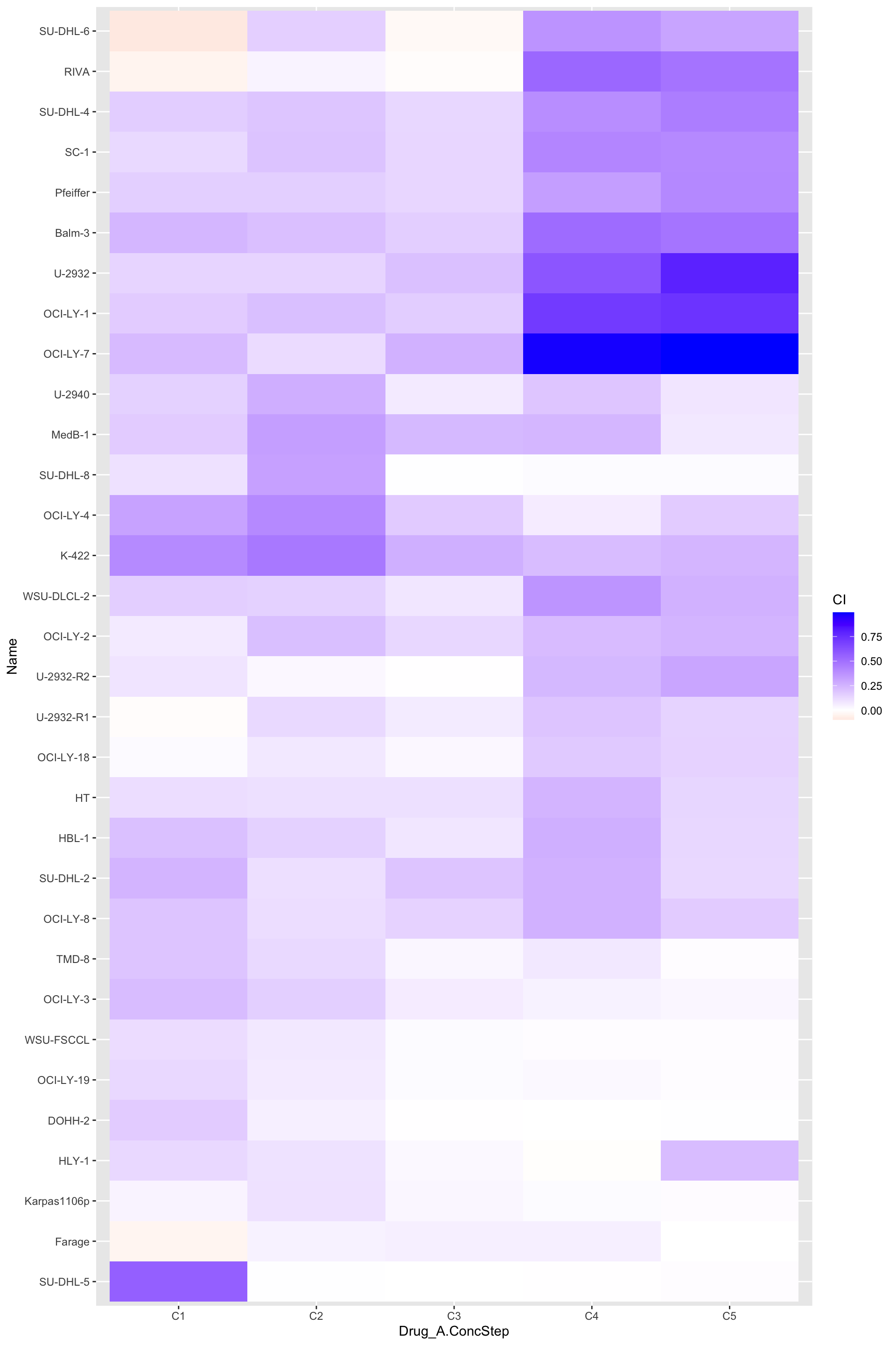 Very few combinatorial effect. Mostly antagonistic
Summarise CI
Calculate synergistic and antagonistic effect separately, using a similar way as bayesyngergy package
sumSyn <- function(viabExp, viabObs) {
  tab <- tibble(viabExp=viabExp, viabObs = viabObs) %>%
    mutate(syn = min(0, viabObs - viabExp),
           anta = max(0, viabObs - viabExp))
  return(tibble(syn = sum(tab$syn), anta = sum(tab$anta)))
}

ciTabSum <- group_by(synTab, Name, Drug_A) %>% nest() %>%
  mutate(res = map(data, ~sumSyn(.$viabExp, .$viabObs))) %>%
  unnest(res) %>% select(-data) %>% arrange(syn) %>%
  mutate(cellName = ifelse(syn<0 | anta > 3,Name,""))
ggplot(ciTabSum, aes(x=syn,y=anta, label = cellName)) +
geom_point() + ggrepel::geom_text_repel() +
xlab("Synergistic score") + ylab("Antagonistic score") 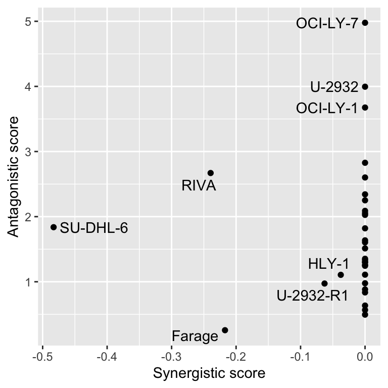
Plot combination curve for each drug, drug are ranked based on the sigificance correlation, cell lines are ranked based on CI
pList <- lapply(unique(ciTabSum$Name), function(eachCell) {
  plotTab <- filter(synTab, Name == eachCell) %>%
    select(Name, Drug_A, Drug_A.ConcStep, viabA, viabB, viabExp, viabObs) %>%
    pivot_longer(-c("Name","Drug_A","Drug_A.ConcStep"), names_to = "type", values_to = "viab") %>%
    mutate(lineType = ifelse(type %in% c("viabA","viabB"), "single","combine"))

  ggplot(plotTab, aes(x=Drug_A.ConcStep, y=viab, group=type)) +
    geom_line(aes(col = type, linetype = lineType)) +
    scale_linetype_manual(values = c(combine = "solid", `single` = "dotted"), name = "combination", guide = "none") +
    scale_color_manual(values =c(viabA = "orange", viabB="darkgreen",
                                 viabExp = "red", viabObs="blue"),
                       labels=c("CHP only ","Pola only","expected effect","observed effect"),
                       name = "treatment") +
    ggtitle(eachCell) +
    ylab("Viability") + xlab("Concentration step")
})
cowplot::plot_grid(plotlist= pList, ncol=3)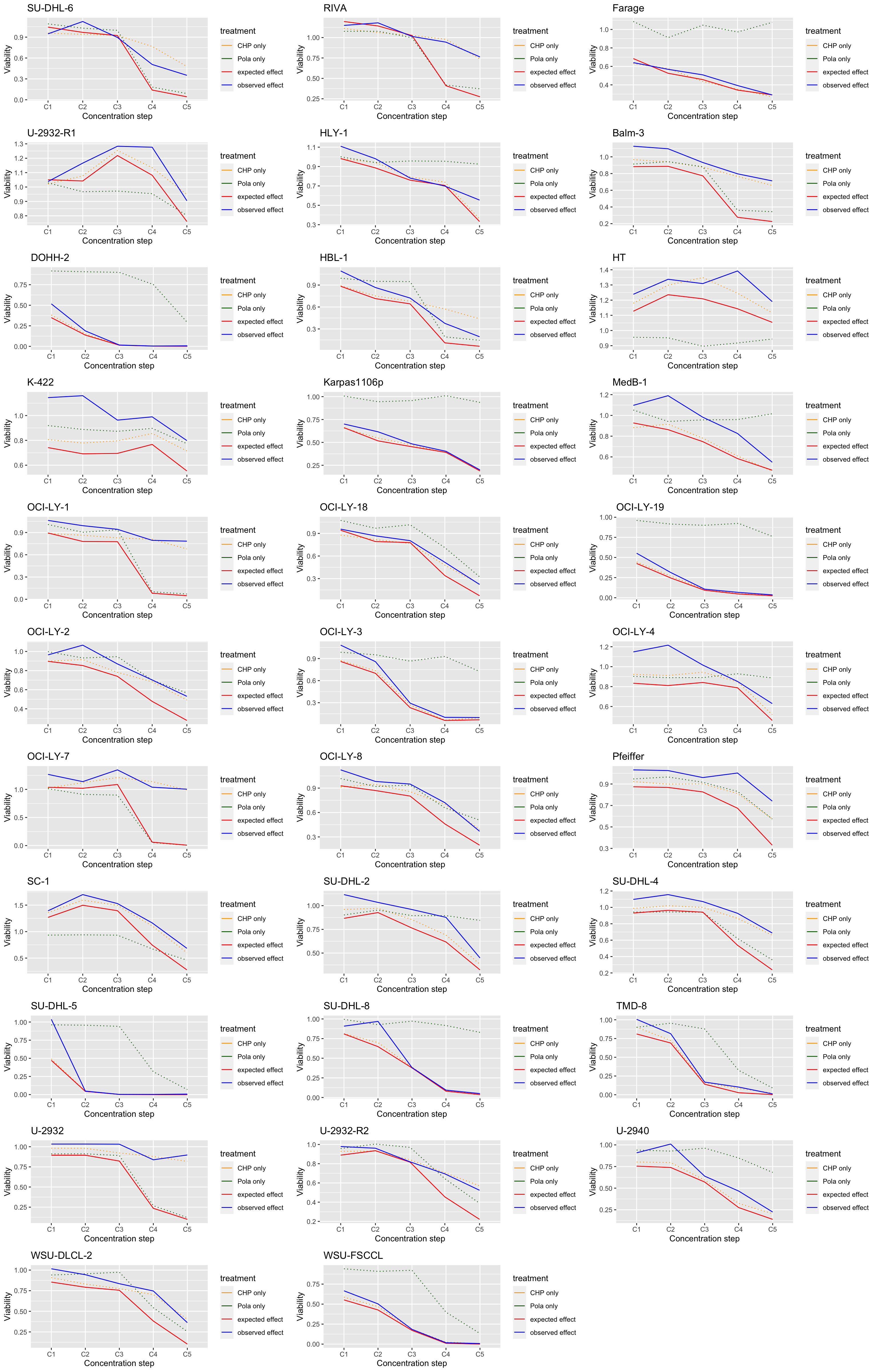
sessionInfo()R version 4.1.2 (2021-11-01)
Platform: x86_64-apple-darwin17.0 (64-bit)
Running under: macOS Big Sur 10.16
Matrix products: default
BLAS: /Library/Frameworks/R.framework/Versions/4.1/Resources/lib/libRblas.0.dylib
LAPACK: /Library/Frameworks/R.framework/Versions/4.1/Resources/lib/libRlapack.dylib
locale:
[1] en_US.UTF-8/en_US.UTF-8/en_US.UTF-8/C/en_US.UTF-8/en_US.UTF-8
attached base packages:
[1] stats graphics grDevices utils datasets methods base
other attached packages:
[1] forcats_0.5.1 stringr_1.4.0 dplyr_1.0.7 purrr_0.3.4
[5] readr_2.1.1 tidyr_1.1.4 tibble_3.1.6 ggplot2_3.3.5
[9] tidyverse_1.3.1
loaded via a namespace (and not attached):
[1] ggrepel_0.9.1 Rcpp_1.0.8 lubridate_1.8.0 assertthat_0.2.1
[5] rprojroot_2.0.2 digest_0.6.29 utf8_1.2.2 R6_2.5.1
[9] cellranger_1.1.0 backports_1.4.1 reprex_2.0.1 evaluate_0.14
[13] highr_0.9 httr_1.4.2 pillar_1.6.5 rlang_0.4.12
[17] readxl_1.3.1 rstudioapi_0.13 jquerylib_0.1.4 rmarkdown_2.11
[21] labeling_0.4.2 munsell_0.5.0 broom_0.7.11 compiler_4.1.2
[25] httpuv_1.6.5 modelr_0.1.8 xfun_0.29 pkgconfig_2.0.3
[29] htmltools_0.5.2 tidyselect_1.1.1 workflowr_1.7.0 fansi_1.0.2
[33] crayon_1.4.2 tzdb_0.2.0 dbplyr_2.1.1 withr_2.4.3
[37] later_1.3.0 grid_4.1.2 jsonlite_1.7.3 gtable_0.3.0
[41] lifecycle_1.0.1 DBI_1.1.2 git2r_0.29.0 magrittr_2.0.1
[45] scales_1.1.1 cli_3.1.1 stringi_1.7.6 farver_2.1.0
[49] fs_1.5.2 promises_1.2.0.1 xml2_1.3.3 bslib_0.3.1
[53] ellipsis_0.3.2 generics_0.1.1 vctrs_0.3.8 cowplot_1.1.1
[57] tools_4.1.2 glue_1.6.1 hms_1.1.1 fastmap_1.1.0
[61] yaml_2.2.1 colorspace_2.0-2 rvest_1.0.2 knitr_1.37
[65] haven_2.4.3 sass_0.4.0