Analysis of combinatorial effect using bayesynergy method

workflowr

• Summary
• Checks
• Past versions

Last updated: 2022-05-20

Checks: 5 1

Knit directory: combiDLBCL/analysis/

This reproducible R Markdown analysis was created with workflowr (version 1.7.0). The Checks tab describes the reproducibility checks that were applied when the results were created. The Past versions tab lists the development history.

---

Environment: empty

Great job! The global environment was empty. Objects defined in the global environment can affect the analysis in your R Markdown file in unknown ways. For reproduciblity it’s best to always run the code in an empty environment.

Seed: set.seed(20220425)

The command set.seed(20220425) was run prior to running the code in the R Markdown file. Setting a seed ensures that any results that rely on randomness, e.g. subsampling or permutations, are reproducible.

Session information: recorded

Great job! Recording the operating system, R version, and package versions is critical for reproducibility.

Cache: none

Nice! There were no cached chunks for this analysis, so you can be confident that you successfully produced the results during this run.

File paths: relative

Great job! Using relative paths to the files within your workflowr project makes it easier to run your code on other machines.

Repository version: no version control

Tracking code development and connecting the code version to the results is critical for reproducibility. To start using Git, open the Terminal and type git init in your project directory.

---

This project is not being versioned with Git. To obtain the full reproducibility benefits of using workflowr, please see ?wflow_start.

---

Load libraries and datasets

Preprocess

Only use CHP_Pola plates

screenSub <- filter(screenData, Drug_B == "CHP_Pola")

Create input

allPair <- distinct(screenSub, Name, Drug_A) %>%
  filter(Drug_A != "DMSO")
allInput <- lapply(seq(nrow(allPair)), function(i) {
  n <- allPair[i,]$Name
  m <- allPair[i,]$Drug_A
  viabTab <- filter(screenSub, Name == n) %>%
    select(Drug_A, Drug_B, Drug_A.Conc, Drug_B.Conc, normVal)
  bTab <- filter(viabTab, Drug_A == "DMSO")
  aTab <- filter(viabTab, Drug_A == m)
  testViab <- bind_rows(aTab, bTab)
  y <- as.matrix(data.frame(viability=testViab$normVal))
  x = as.matrix(testViab[,c("Drug_A.Conc","Drug_B.Conc")])
  list(y=y, x=x, drug_names = c(m,n), experiment_ID = paste0(n,"_",m))
})

Fit bayesynergy model

fit <- synergyscreen(allInput, save_raw = F, save_plots = F, bayesynergy_params = list(method = "vb"))
save(fit, file = "../output/fit.RData")

Load previous results (fitting takes long time)

load("../output/fit.RData")

Get the result table

allRes <- fit$screenSummary
ciTabBayes <- tibble(Name = allRes$`Drug B`,
                 Drug_A = allRes$`Drug A`, 
                 syn = allRes$`Synergy (mean)`,
                 anta = allRes$`Antagonism (mean)`
                 #syn = allRes$`Synergy Score`,
                 #anta = allRes$`Antagonism Score`
                 )

Visualization of synergistic and antagoistic effect

Scatter plot

plotSynScatter(ciTabBayes, 0.05)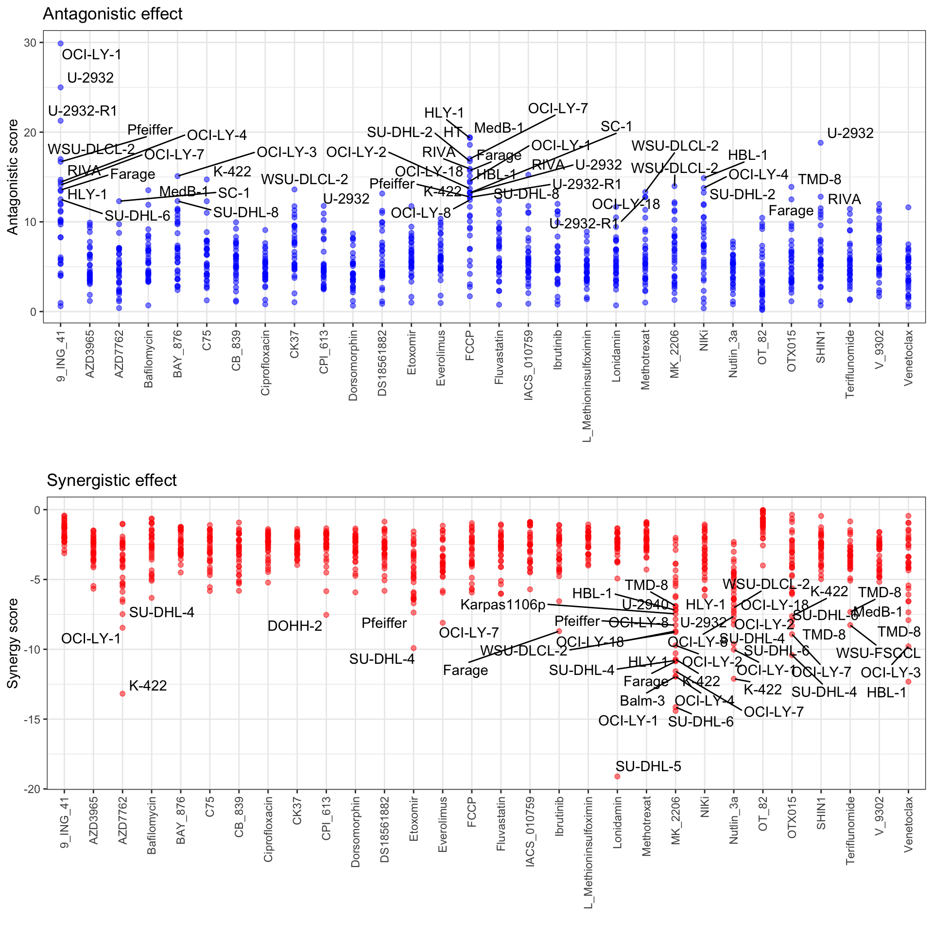

Matrix visualization

plotSynMatrix(ciTabBayes, 0.1, 0.2)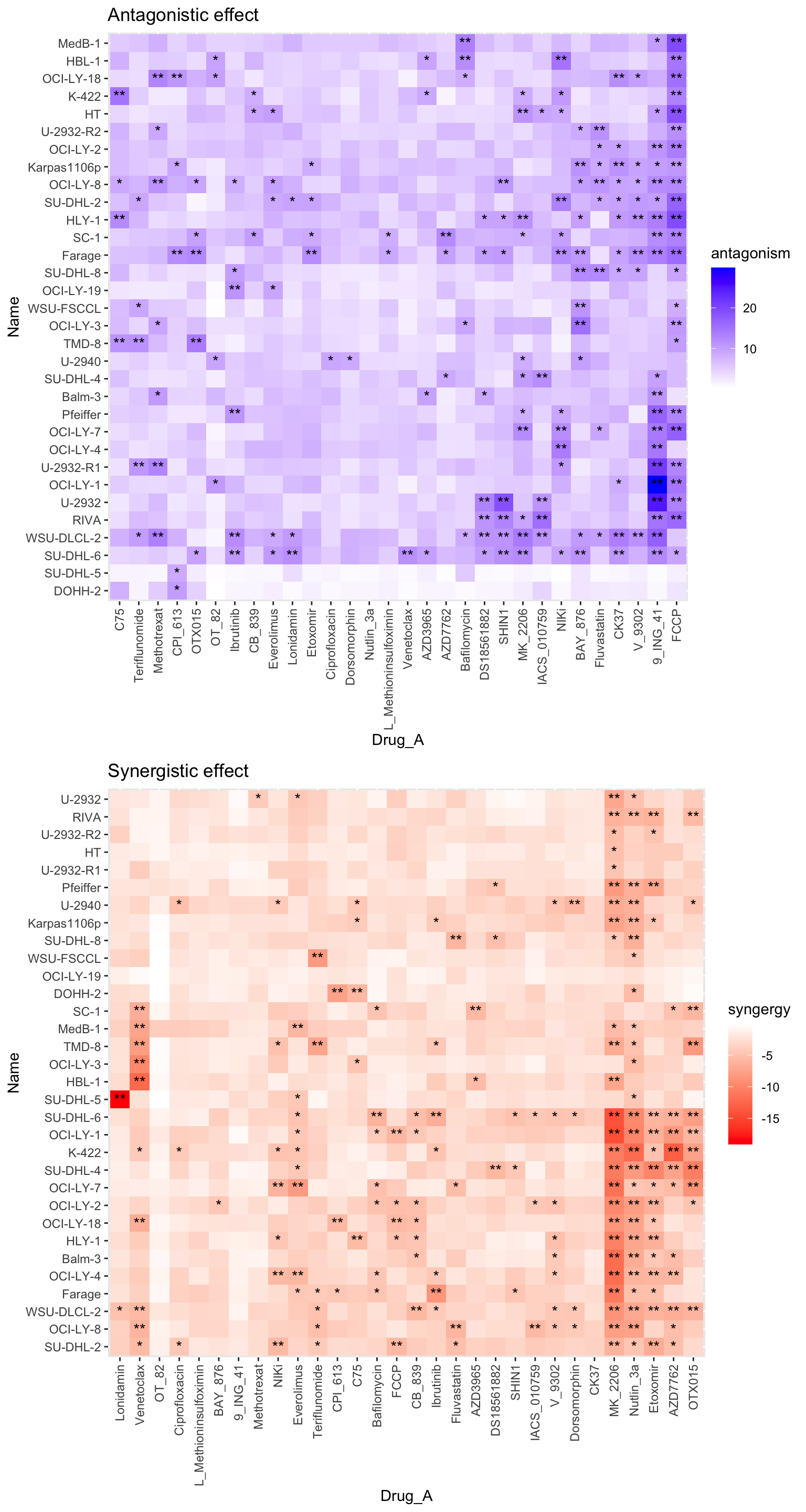

Correlate summarised CI to the single angent response of CHP_Pola

Add single agent CHP_Pola or CHOP response

polaTab <- screenData %>% filter(Drug_A == "DMSO", Drug_B == "CHP_Pola",!ifEdge) %>%
  group_by(Name) %>% summarise(viabPola = mean(normVal))

Test for correlation

testTab <- left_join(ciTabBayes, polaTab, by = "Name") %>%
  pivot_longer(c("viabPola"), names_to = "Drug_B", values_to = "viab") %>%
  pivot_longer(c("syn","anta"), names_to = "effect", values_to = "score")

resTab <- group_by(testTab, Drug_A, Drug_B, effect) %>% nest() %>%
  mutate(m=map(data, ~cor.test(~score+viab,.))) %>%
  mutate(res = map(m, broom::tidy)) %>%
  unnest(res) %>%
  select(Drug_A, Drug_B, estimate, p.value, effect) %>%
  ungroup() %>% group_by(effect) %>%
  mutate(p.adj = p.adjust(p.value, method = "BH")) %>%
  arrange(p.value)

Correlation with synergistic

resTab.syn <- filter(resTab, p.adj <0.1, effect == "syn")
pList <- lapply(seq(nrow(resTab.syn)), function(i) {
  rec <- resTab.syn[i,]
  plotTab <- filter(testTab, Drug_A == rec$Drug_A, Drug_B==rec$Drug_B, effect == rec$effect)
  ggplot(plotTab, aes(x=viab, y=score, label = Name)) +
    geom_point(aes(col=Name)) +
    geom_smooth(method = "lm",se=FALSE) +
    ggrepel::geom_text_repel() +
    theme(legend.position = "none") +
    xlab(rec$Drug_B) + ylab("average CI") +
    ggtitle(sprintf("%s\n(p=%s, coef=%s)",rec$Drug_A, formatC(rec$p.value, digits = 2),formatC(rec$estimate, digits = 1)))
})
cowplot::plot_grid(plotlist=pList)

`geom_smooth()` using formula 'y ~ x'
`geom_smooth()` using formula 'y ~ x'
`geom_smooth()` using formula 'y ~ x'
`geom_smooth()` using formula 'y ~ x'
`geom_smooth()` using formula 'y ~ x'
`geom_smooth()` using formula 'y ~ x'
`geom_smooth()` using formula 'y ~ x'
`geom_smooth()` using formula 'y ~ x'

Warning: ggrepel: 1 unlabeled data points (too many overlaps). Consider increasing max.overlaps
ggrepel: 1 unlabeled data points (too many overlaps). Consider increasing max.overlaps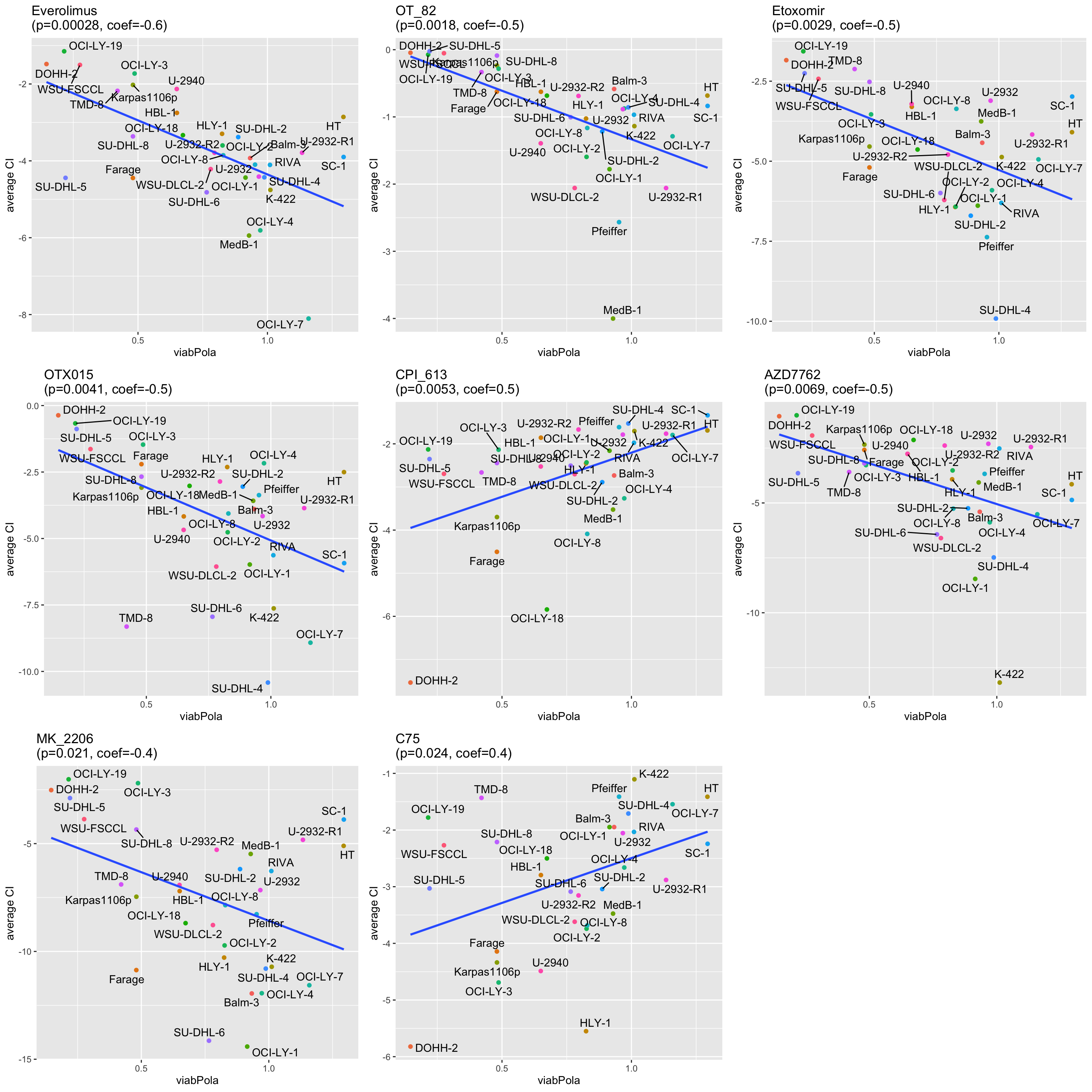

Correlation with antagonistic

resTab.anta <- filter(resTab, p.adj <0.1, effect == "anta")
pList <- lapply(seq(nrow(resTab.anta)), function(i) {
  rec <- resTab.anta[i,]
  plotTab <- filter(testTab, Drug_A == rec$Drug_A, Drug_B==rec$Drug_B, effect == rec$effect)
  ggplot(plotTab, aes(x=viab, y=score, label = Name)) +
    geom_point(aes(col=Name)) +
    geom_smooth(method = "lm",se=FALSE) +
    ggrepel::geom_text_repel() +
    theme(legend.position = "none") +
    xlab(rec$Drug_B) + ylab("average CI") +
    ggtitle(sprintf("%s\n(p=%s, coef=%s)",rec$Drug_A, formatC(rec$p.value, digits = 2),formatC(rec$estimate, digits = 1)))
})
cowplot::plot_grid(plotlist=pList)

`geom_smooth()` using formula 'y ~ x'
`geom_smooth()` using formula 'y ~ x'
`geom_smooth()` using formula 'y ~ x'
`geom_smooth()` using formula 'y ~ x'
`geom_smooth()` using formula 'y ~ x'
`geom_smooth()` using formula 'y ~ x'
`geom_smooth()` using formula 'y ~ x'
`geom_smooth()` using formula 'y ~ x'
`geom_smooth()` using formula 'y ~ x'
`geom_smooth()` using formula 'y ~ x'
`geom_smooth()` using formula 'y ~ x'
`geom_smooth()` using formula 'y ~ x'
`geom_smooth()` using formula 'y ~ x'
`geom_smooth()` using formula 'y ~ x'
`geom_smooth()` using formula 'y ~ x'

Warning: ggrepel: 13 unlabeled data points (too many overlaps). Consider
increasing max.overlaps

Warning: ggrepel: 16 unlabeled data points (too many overlaps). Consider
increasing max.overlaps

Warning: ggrepel: 12 unlabeled data points (too many overlaps). Consider
increasing max.overlaps

Warning: ggrepel: 13 unlabeled data points (too many overlaps). Consider
increasing max.overlaps

Warning: ggrepel: 11 unlabeled data points (too many overlaps). Consider
increasing max.overlaps

Warning: ggrepel: 8 unlabeled data points (too many overlaps). Consider
increasing max.overlaps

Warning: ggrepel: 17 unlabeled data points (too many overlaps). Consider
increasing max.overlaps

Warning: ggrepel: 15 unlabeled data points (too many overlaps). Consider increasing max.overlaps
ggrepel: 15 unlabeled data points (too many overlaps). Consider increasing max.overlaps

Warning: ggrepel: 16 unlabeled data points (too many overlaps). Consider
increasing max.overlaps

Warning: ggrepel: 13 unlabeled data points (too many overlaps). Consider
increasing max.overlaps

Warning: ggrepel: 14 unlabeled data points (too many overlaps). Consider
increasing max.overlaps

Warning: ggrepel: 11 unlabeled data points (too many overlaps). Consider
increasing max.overlaps

Warning: ggrepel: 12 unlabeled data points (too many overlaps). Consider
increasing max.overlaps

Warning: ggrepel: 8 unlabeled data points (too many overlaps). Consider
increasing max.overlaps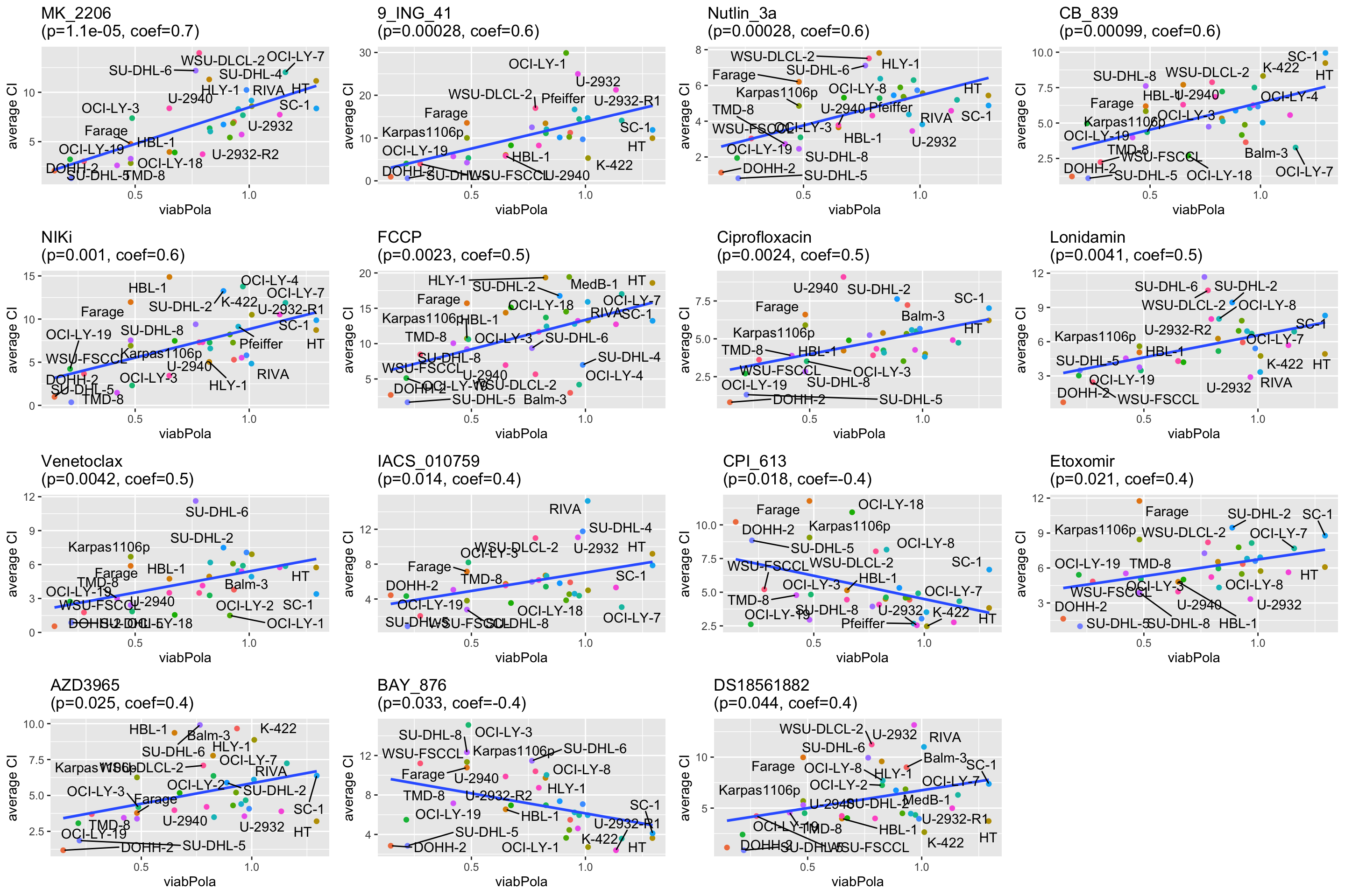

Test for synergistic effect related to genomics

Preprocess genomics

load("../data/SVs_filtered.RData")

mutTab <- svTab %>% filter(Name %in% ciTabBayes$Name) %>%
  group_by(Name, Gene) %>% summarise(n = length(Name)) %>%
  arrange(desc(n))

`summarise()` has grouped output by 'Name'. You can override using the
`.groups` argument.

#Get mutations occured at least in three cell lines
geneCount <- group_by(mutTab, Gene) %>% summarise(n=length(Name)) %>%
  filter(n>=3) %>% arrange(desc(n)) 

mutTab <- filter(mutTab, Gene %in% geneCount$Gene) %>%
  mutate(status =1) %>% select(Name, Gene, status) %>%
  pivot_wider(names_from = "Gene", values_from = "status") %>%
  mutate_all(replace_na,0) %>%
  pivot_longer(-Name, names_to = "Gene", values_to = "status")

`mutate_all()` ignored the following grouping variables:
• Column `Name`
ℹ Use `mutate_at(df, vars(-group_cols()), myoperation)` to silence the message.

T-test

testTab <- ciTabBayes %>% full_join(mutTab, by = "Name") %>%
  pivot_longer(c("syn","anta"), names_to = "effect", values_to = "CI") %>%
  filter(!is.na(Gene),!is.na(CI), effect =="syn")

resTab <- group_by(testTab, Drug_A, Gene, effect) %>% nest() %>%
  mutate(m = map(data, ~t.test(CI ~ status,., var.equal=TRUE))) %>%
  mutate(res = map(m, broom::tidy)) %>%
  unnest(res) %>%
  select(Drug_A, Gene, effect, estimate, p.value) %>%
  arrange(p.value) %>% ungroup() %>%
  mutate(p.adj = p.adjust(p.value, method = "BH"))

resTab.sig <- filter(resTab, p.adj <= 0.1)
hist(resTab$p.value)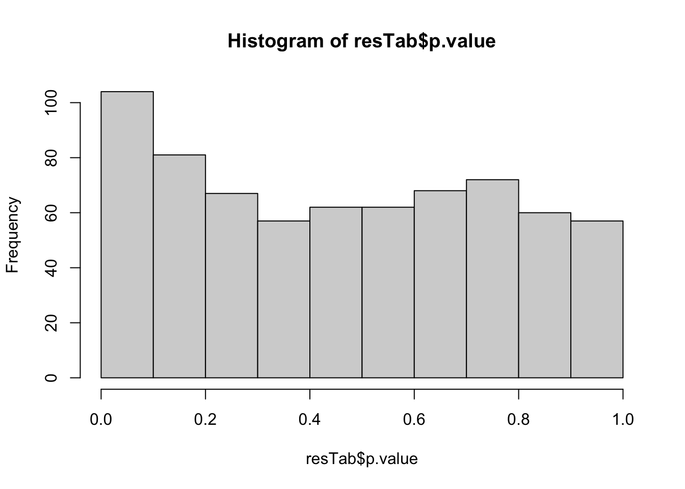

Boxplots for associations passed 10% FDR

pList <- lapply(seq(nrow(resTab.sig)), function(i) {
  rec <- resTab.sig[i,]
  plotTab <- filter(testTab, Drug_A == rec$Drug_A, Gene == rec$Gene, effect == rec$effect) %>%
    mutate(status = factor(status))
  ggplot(plotTab, aes(x=status, y=CI)) +
    geom_boxplot(aes(fill = status)) +
    geom_point() +
    ggtitle(sprintf("%s ~ %s (p=%s)",rec$Drug_A, rec$Gene, formatC(rec$p.value, digits = 2))) +
    xlab(rec$Gene) +
    theme_bw() +
    theme(legend.position = "none")
})

cowplot::plot_grid(plotlist = pList, ncol=4)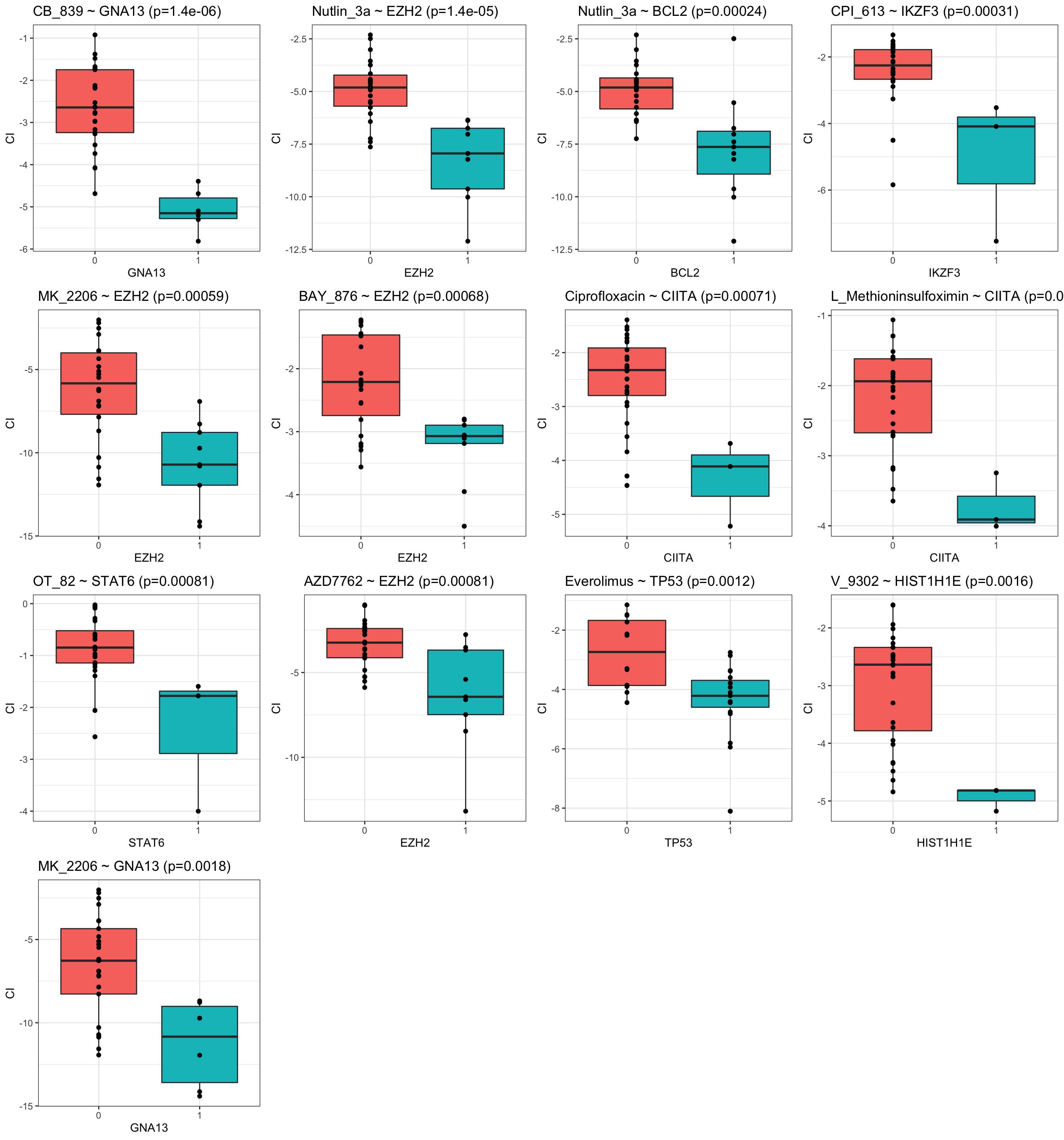

Heatmap

library(pheatmap)
ciTab <- testTab %>% 
  filter(Gene %in% resTab.sig$Gene, Drug_A %in% resTab.sig$Drug_A)

ciMat <- distinct(ciTab, Name, Drug_A, CI) %>%
  pivot_wider(names_from = "Name", values_from = "CI") %>%
  column_to_rownames("Drug_A") %>% as.matrix()

colAnno <- ciTab %>% ungroup() %>% distinct(Name, Gene, status) %>%
  mutate(status = as.character(status)) %>%
  pivot_wider(names_from = "Gene", values_from = "status") %>%
  column_to_rownames("Name")
annoColor <- lapply(colnames(colAnno), function(x) {c("1"="black","0"="white")})
names(annoColor) <- colnames(colAnno)
pheatmap(ciMat, annotation_col = colAnno, annotation_colors = annoColor)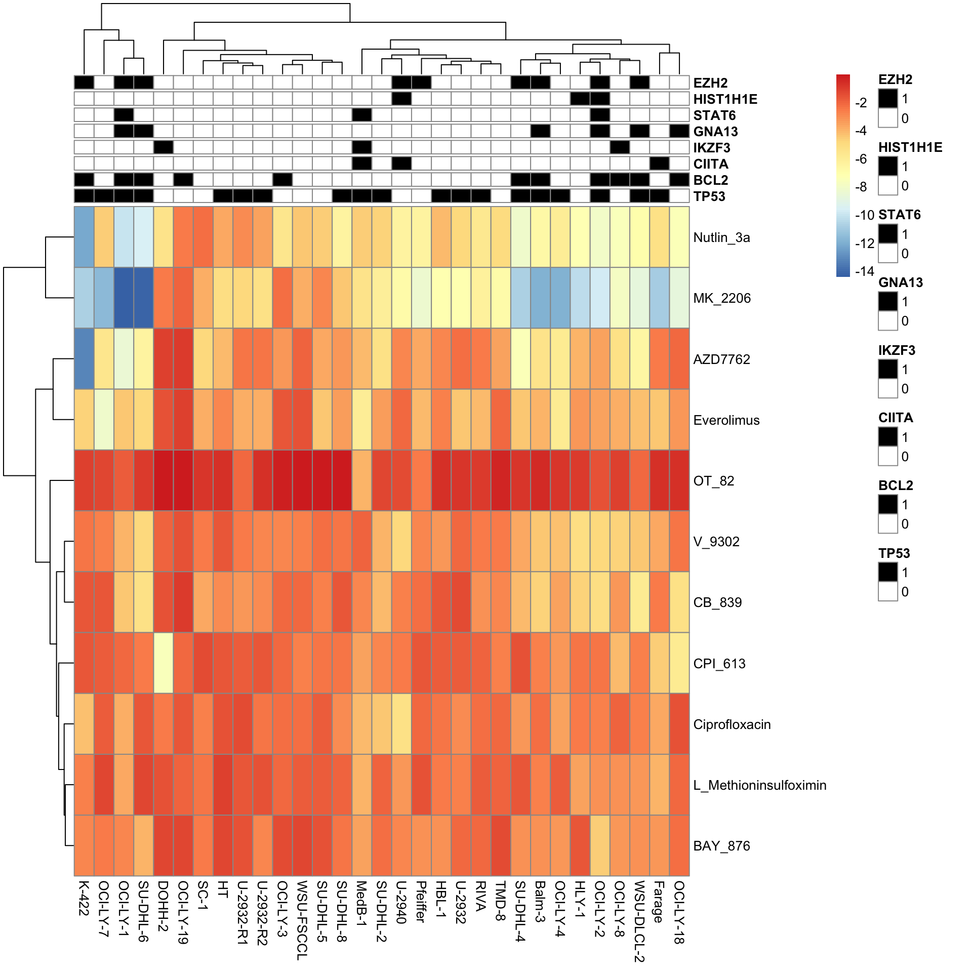

Session information

sessionInfo()

R version 4.2.0 (2022-04-22)
Platform: x86_64-apple-darwin17.0 (64-bit)
Running under: macOS Big Sur/Monterey 10.16

Matrix products: default
BLAS:   /Library/Frameworks/R.framework/Versions/4.2/Resources/lib/libRblas.0.dylib
LAPACK: /Library/Frameworks/R.framework/Versions/4.2/Resources/lib/libRlapack.dylib

locale:
[1] en_US.UTF-8/en_US.UTF-8/en_US.UTF-8/C/en_US.UTF-8/en_US.UTF-8

attached base packages:
[1] stats     graphics  grDevices utils     datasets  methods   base     

other attached packages:
 [1] pheatmap_1.0.12   bayesynergy_2.4.1 forcats_0.5.1     stringr_1.4.0    
 [5] dplyr_1.0.9       purrr_0.3.4       readr_2.1.2       tidyr_1.2.0      
 [9] tibble_3.1.7      ggplot2_3.3.6     tidyverse_1.3.1  

loaded via a namespace (and not attached):
  [1] colorspace_2.0-3     ellipsis_0.3.2       ggridges_0.5.3      
  [4] rgdal_1.5-30         rprojroot_2.0.3      fs_1.5.2            
  [7] rstudioapi_0.13      farver_2.1.0         rstan_2.21.5        
 [10] ggrepel_0.9.1        fansi_1.0.3          mvtnorm_1.1-3       
 [13] lubridate_1.8.0      xml2_1.3.3           splines_4.2.0       
 [16] bridgesampling_1.1-2 codetools_0.2-18     doParallel_1.0.17   
 [19] knitr_1.39           jsonlite_1.8.0       workflowr_1.7.0     
 [22] Cairo_1.5-15         broom_0.8.0          dbplyr_2.1.1        
 [25] compiler_4.2.0       httr_1.4.3           backports_1.4.1     
 [28] assertthat_0.2.1     Matrix_1.4-1         fastmap_1.1.0       
 [31] lazyeval_0.2.2       cli_3.3.0            later_1.3.0         
 [34] htmltools_0.5.2      prettyunits_1.1.1    tools_4.2.0         
 [37] igraph_1.3.1         coda_0.19-4          gtable_0.3.0        
 [40] glue_1.6.2           inlmisc_0.5.5        Rcpp_1.0.8.3        
 [43] cellranger_1.1.0     jquerylib_0.1.4      raster_3.5-15       
 [46] vctrs_0.4.1          nlme_3.1-157         iterators_1.0.14    
 [49] xfun_0.31            ps_1.7.0             rvest_1.0.2         
 [52] lifecycle_1.0.1      terra_1.5-21         scales_1.2.0        
 [55] hms_1.1.1            doSNOW_1.0.20        promises_1.2.0.1    
 [58] Brobdingnag_1.2-7    parallel_4.2.0       inline_0.3.19       
 [61] RColorBrewer_1.1-3   yaml_2.3.5           gridExtra_2.3       
 [64] loo_2.5.1            StanHeaders_2.21.0-7 sass_0.4.1          
 [67] stringi_1.7.6        highr_0.9            foreach_1.5.2       
 [70] pkgbuild_1.3.1       rlang_1.0.2          pkgconfig_2.0.3     
 [73] matrixStats_0.62.0   evaluate_0.15        lattice_0.20-45     
 [76] htmlwidgets_1.5.4    labeling_0.4.2       cowplot_1.1.1       
 [79] tidyselect_1.1.2     processx_3.5.3       plyr_1.8.7          
 [82] magrittr_2.0.3       R6_2.5.1             snow_0.4-4          
 [85] generics_0.1.2       DBI_1.1.2            mgcv_1.8-40         
 [88] pillar_1.7.0         haven_2.5.0          withr_2.5.0         
 [91] sp_1.4-7             modelr_0.1.8         crayon_1.5.1        
 [94] utf8_1.2.2           plotly_4.10.0        tzdb_0.3.0          
 [97] rmarkdown_2.14       grid_4.2.0           readxl_1.4.0        
[100] data.table_1.14.2    callr_3.7.0          git2r_0.30.1        
[103] reprex_2.0.1         digest_0.6.29        httpuv_1.6.5        
[106] RcppParallel_5.1.5   stats4_4.2.0         munsell_0.5.0       
[109] viridisLite_0.4.0    bslib_0.3.1